Bridging text spotting and SLAM with junction features
The MIT Faculty has made this article openly available.
Please share
how this access benefits you. Your story matters.
Citation
Wang, Hsueh-Cheng, Chelsea Finn, Liam Paull, Michael Kaess, Ruth
Rosenholtz, Seth Teller, and John Leonard. “Bridging Text Spotting
and SLAM with Junction Features.” 2015 IEEE/RSJ International
Conference on Intelligent Robots and Systems (IROS) (September
2015). ©2015 Institute of Electrical and Electronics Engineers (IEEE)
As Published
http://dx.doi.org/10.1109/IROS.2015.7353895
Publisher
Institute of Electrical and Electronics Engineers (IEEE)
Version
Author's final manuscript
Citable link
http://hdl.handle.net/1721.1/107466
Terms of Use
Creative Commons Attribution-Noncommercial-Share Alike
Bridging Text Spotting and SLAM with Junction Features
Hsueh-Cheng Wang
1, Chelsea Finn
2, Liam Paull
1, Michael Kaess
3Ruth Rosenholtz
1, Seth Teller
1, and John Leonard
1hchengwang,lpaull,rruth,[email protected], [email protected], [email protected]
Abstract— Navigating in a previously unknown environment and recognizing naturally occurring text in a scene are two important autonomous capabilities that are typically treated as distinct. However, these two tasks are potentially complemen-tary, (i) scene and pose priors can benefit text spotting, and (ii) the ability to identify and associate text features can benefit navigation accuracy through loop closures. Previous approaches to autonomous text spotting typically require significant train-ing data and are too slow for real-time implementation. In this work, we propose a novel high-level feature descriptor, the “junction”, which is particularly well-suited to text represen-tation and is also fast to compute. We show that we are able to improve SLAM through text spotting on datasets collected with a Google Tango, illustrating how location priors enable improved loop closure with text features.
I. INTRODUCTION
Autonomous navigation and recognition of environmental text are two prerequisites for higher level semantic under-standing of the world that are normally treated as distinct. Simultaneous localization and mapping (SLAM) has been extensively studied for almost 30 years (For an overview see [1]). Automatic environmental text recognition has seen comparatively less research attention but has been the subject of more recent studies (For example [2]–[13] among others). The ability to recognize text in the environment is invaluable from a semantic mapping perspective [14]. One important potential application (among many) is to provide navigation assistance to the visually impaired. Text provides important cues for navigating and performing tasks in the environment such as walking to the elevator and selecting the correct floor. Recent graphical approaches in SLAM have shown the ability to produce accurate trajectory and map estimates in real-time for medium to large scale problems [15]. However, the same cannot be said for state-of-the-art environmental text spotting algorithms. Unlike scanning documents, envi-ronmental text often occurs in only a tiny portion of the entire sensor field of view (FOV). As a result, the obtained obser-vations often lack enough pixels for resolution-demanding text decoding. Additionally, scene text is highly variable in terms of font, color, scale, and aspect. Motion and out-of-focus blurry inputs from moving cameras result in further
This work was supported by the Andrea Bocelli Foundation, the East Japan Railway Company, the Office of Naval Research under grants N00014-10-1-0936, N00014-11-1-0688 and N00014-13-1-0588, and by NSF Award IIS-1318392.
1Computer Science and Artificial Intelligence Laboratory, Massachusetts
Institute of Technology, Cambridge, MA, USA;2Electrical Engineering and
Computer Sciences, UC Berkeley;3 Robotics Institute, Carnegie Mellon University
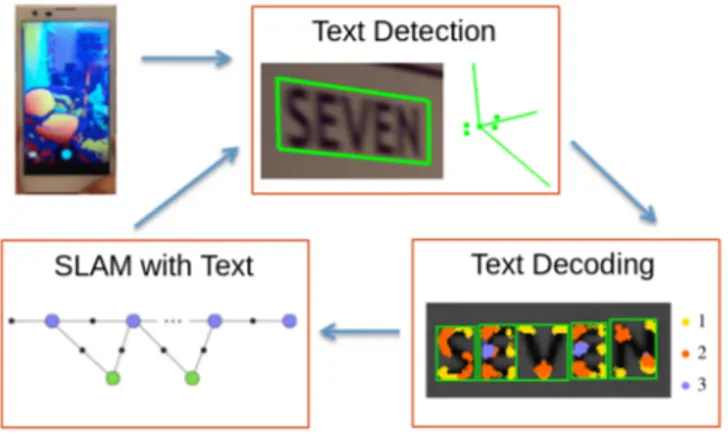
Fig. 1. Integrated SLAM and text spotting: Raw sensor input from the Google Tango device is combined with the output of the SLAM solver to generate a prior for “Text Detection”. This representation enables SLAM to be recognized and used to add loop closure constraints in a SLAM system.
challenges. Furthermore, the state-of-the-art deep-learning approaches [16]–[18] typically evaluate more than 50,000 region proposals, which cost significant prediction time that is incompatible with real-time deployment.
In this work, we address these shortcomings through the development of a new descriptor, termed a “junction”, that is particularly well-suited to the text spotting tasks and is fast enough to enable integration into a real-time SLAM system. We propose to merge the SLAM and text spotting tasks into one integrated system. Specifically, if scene text can be reliably identified, it can be used as a landmark within a SLAM system to improve localization. Conversely, with access to a prior on the camera pose and 3D scene information from SLAM, text can more efficiently be detected and identified
To summarize, the contributions of this work are: 1) A new representation for text that is able to quickly
reject non-text region proposals, and match candidate region proposals to words in a task-relevant lexicon; 2) To extract text quickly and accurately enough to
sup-port real-time decision-making and full integration into a SLAM system, thereby improving the camera pose and scene estimates through loop closure.
An overview of the approach is shown in Figure 1. We use the Google Tango device for experiments, which provides an integrated visual inertial odometry (VIO) estimate as well as depth sensor output. The raw sensor data is combined with the output of the SLAM system to predict the perspective
transformation of the text since it usually appears on planar surfaces in the scene. This information is used to separate the word into individual characters. The junction features are built for each character (details in Sec. III). The discovered characters are matched against existing words in the lexicon (dictionary) and measurements are added to the SLAM graph (details Sec. IV).
II. RELATEDWORK
In this section we focus on related research in the field of text spotting, with a particular focus on work related to navigation and mapping. For a review of SLAM results we refer the reader to [1]. In our approach we leverage more recent efficient graphical approaches to solving the full SLAM problem (entire robot trajectory and map) which are described in [15], [19], [20].
A. Environmental Text Spotting
Text spotting algorithms typically start with extracting features (keypoints, edges, strokes, and blobs) in order to distinguish text from other texture types. Some corner feature detectors have been shown to be particularly successful for this task, such as Harris corners [21] as used by Zhao et al. [22]. An alternative is to consider edges since text is typically composed of strokes with strong gradients on both sides. Edge-based methods are effective when the background is relatively plain; however, in real-world scenes, strong edges are very common so extra effort should be devoted to reducing false positives. For example, inspired by face and pedestrian detectors [23], Histogram of Oriented Gradients (HOG) based approaches include edge orientation or spatial information, and perform multi-scale character detection via sliding window classification [2]–[4]. However, due to the large search space, at present HOG-based approaches are too computationally expensive for real-time implementation. Another common feature used is stroke width and orientation (e.g. [24], [25]). One such method uses the assumption of nearly constant stroke width to transform and filter the input [26]. Similar to edge-based methods, stroke-based ap-proaches can produce an intolerable number of false positives in the presence of regular textures such as brick walls or fences.
Neumann and Matas [5]–[7] used extremal regions (ERs) to extract candidate blobs and shape descriptors. In [5], an efficient detection algorithm was reported using two classifiers of sequential selection from ERs. This method is now publicly available and state-of-the-art in terms of efficiency [8]. However, ER alone is insufficient for full end-to-end text spotting since a robust decoding method is still required.
Instead of hand-designed features, a visual dictionary learning approach has been proposed to extract mid-level features and their associations for decoding (classification) problems. Such work was introduced in object detection as “sketch tokens” [27]. A similar approach has been ap-plied to text spotting by combining Harris corners with an appearance and structure model [28]. Lee et al. [10]
proposed a multi-class classification framework using region-based feature pooling for scene character classification and scene text recognition tasks. In [11], “strokelets”, or essential substructures of characters, were learned from labelled text regions and subsequently used to identify text. One notable downside to the dictionary learning approach is that it relies on large amounts of labelled data and may be limited due to the lack of a representative dataset. For example, degraded or warped text observed from a moving camera can cause missed detections.
Recently, deep learning approaches have been applied to text spotting problems and have obtained top results on major benchmark datasets [16]–[18]. Such methods rely on massive labelled training data and have high computational resource requirements. For example, the PhotoOCR [12] system extracts features with a fully-connected network of five hidden layers (422-960-480-480-480-480-100) trained with ≈1.1×10⁷ training samples containing low-resolution and blurry inputs. The system operates at 600 ms/image on average with processing offloaded to the cloud. Instead of collecting and labeling real data, there are also attempts to produce highly realistic synthetic text for training data augmentation [29].
An end-to-end text spotting system is usually tuned to high recall in the detection stage, and then rejects false positives in the decoding (recognition) stage. The key for real-time text spotting is to efficiently and effectively reduce the number of region proposals for later more computationally expensive decoding. Here, we develop methods that exploit the structure inherent in characters and text to increase prediction speed.
B. Using Text to Support Navigation
Although the extraction of text has been investigated extensively, there has been less work on the challenge of performing robotic deployments of text-spotting with nav-igation objectives. Perhaps the first to deploy a real robot to identify text was Posner et al. [30], who proposed to “query” the world and interpret the subject of the scene using environmental text. They trained a cascade of boosted classifiers to detect text regions, which were then converted into words by an optical character recognition (OCR) engine and a generative model. Subsequently, Case et. al. [31] used automatically detected room numbers and names on office signs for semantic mapping. They trained a classifier with a variety of text features, including local variance, edge density, and horizontal and vertical edge strength, in 10 × 10 windows. An OCR was then used to decode candidates into words. Rogers et al. [32] proposed to detect high-level landmarks, such as door signs, objects, and furniture, for robot navigation. The detected landmarks are then used for data association and loop closure. They first detected visually salient regions, and then trained an SVM classifier using the HOG features. They used the Tesseract OCR software [33] to obtain semantic information. In our work, we do not require extensive training data for classification. A more closely related approach is that of Samarabandu and Liu [34] who
use an edge-based algorithm to extract text. However, this approach is not incorporated into a SLAM system.
C. Using Navigation to Support Text Spotting
In our previous work [13], we proposed to use SLAM to extract planar tiles representing scene surfaces. We integrated multiple observations of each tile from different observer poses. Subsequently, text is detected using the Discrete Cosine Transform (DCT) and ER methods [5], and then the multiple observations are decoded by an OCR engine. The results showed an improved confidence in word recovery in the end-to-end system. The focus of [13] is on fusing multi-ple consecutive text detections to yield a higher confidence result. Here, we use the SLAM and scene information, as well as the junction features described below, to reduce the number of region proposals and therefore improve the overall efficiency.
III. THE PROPOSED JUNCTION FEATURES Similar to many other robotic vision tasks, discovering a good representation for text is critical. We adopt the notion of “junctions” as locations where one or more oriented line segments terminate. For example, an image patch containing the character “E” typically holds one T-shaped (“`”), two L-shaped (“L” and its inversion), and three terminal junc-tions (the horizontal segments). Text in a written system is designed explicitly as a certain combination of strokes, and therefore the intersections and corners in letters are highly constrained. For instances, there are more L-, T- or X-junctions in Chinese; curves and upside-down T-junction and its variants are likely to appear in Arabic; English text lies somewhat in between. The key insight is that junctions occur frequently in text, are robustly detectable, and allow a sufficiently discriminative representation of text.
Junctions in text tend to share common characteristics and become useful properties for text spotting.
1) The pointing direction: the upper one third partitions are typically pointing down and the lower ones other-wise.
2) junctions are highly constrained and can be explicitly designed for a given written system or lexicon. A. Junction Detection
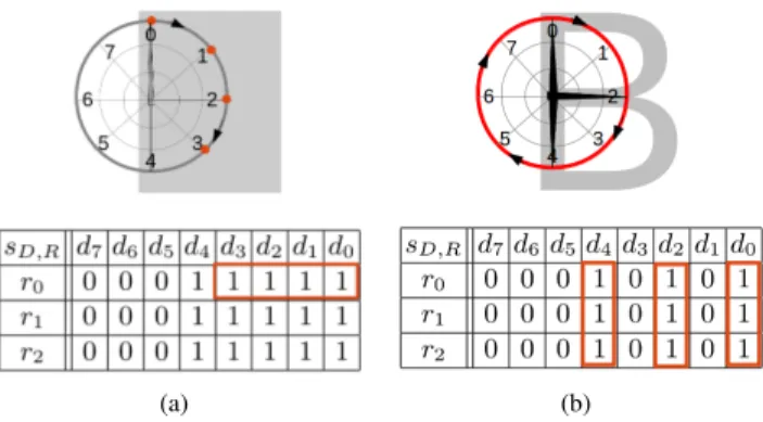
In order to detect junctions, we propose a locally discrimi-native image operator which produces a mid-level descriptor, the “junction binary pattern (JBP).” This process is shown in more detail in Figure 2. The JBP represents the combination of oriented line segments emanating from the center of an image patch. The output is either 0 (non-junction) or an N -digit binary number, where N is the total number of orientations (N = 8 in Figure 2). JBPs are a variant of local binary patterns [35], and are performed on multiple scales with a way to reject a non-junctions quickly. JBPs are also a “simplified” log-polar representation, such as shape contexts [36] or self-similarity descriptors [37] in order to limit the dimensions of representation. In contrast with the SIFT descriptor [38], which uses a histogram of eight bins
(a) (b)
Fig. 2. The junction binary pattern: The algorithm loops clockwise from direction d0 to d7, testing intensity variation between sD,R and nucleus
at 3 different radii, r0 to r2. When the intensities of sD,R and nucleus
are similar, sD,R is labelled as 1. (a) The test terminates early, declaring
a partially or fully uniform patch when a number of consecutive 1’s are found (orange dots). (b) Each direction diis assigned either 0 or 1 when
sdi,r0, sdi,r1, and sdi,r2are all labelled as 1; the detected “`” is encoded
as 00010101.
with varying magnitudes in each direction, our operator describes the combination of two or more oriented line segments to describe patterns of interest.
The center of the image patch is known as the “nucleus” [39]. For a nucleus pixel p and a set of pixels sD,R
sur-rounding p at a distance of R pixels away in each direction D = d0, . . . , dN −1, we test the intensity variation between
Ip and Isdi,R, where Ip is the intensity of the nucleus. If
|Ip−Isdi,R| is smaller than a given threshold, sdi,Ris labelled
as 1, otherwise 0. The testing starts from sd0,R to sdN −1,R
and continues looping clockwise. This process is repeated at M different scales: R = r0..M.
The method is designed to efficiently reject non-junctions, like FAST [40], using computationally inexpensive tests. As shown in Figure 2(a), the loop terminates early to discard partially or fully uniform patches when several consecutive 1’s are detected.
When sdi,r0..M are all labelled 1, the bit corresponding to
direction D = di is assigned as 1, otherwise it is set to 0.
The resulting sequence, D = d0, . . . , dN −1, is encoded as
a binary number (the JBP). For example, the sideways “T” junction ( T) in the character “B” in Figure 2(b) is encoded as the byte 00010101.
In our implementation, we use a Gaussian pyramid with four levels with the radius r0 in each pyramid level. We
found values of 30 for region proposal height, a value of N = 16, and an initial radius, r0= 7 pixels produced good
results for upper case English letters.
IV. END-TO-END SYSTEM WITH SLAM AND TEXT SPOTTING INTEGRATION
In this section we describe the full integration of the text spotting pipeline into a graphical SLAM back-end. We introduce two implementations to refine region proposals efficiently: 1) sliding window using junction features and 2) segmentation with ERs and scene priors. Since the decoding time is essentially proportional to the number of region proposals, we wish to reduce that number and retain high
(a) (b)
(c) (d)
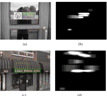
Fig. 3. Examples of detection results in ICDAR and SVT datasets. (a) Grayscale original image from the ICDAR dataset, with detected junctions overlayed. The green rectangle shows a region proposal. The blue dashed rectangle indicates a rejected scan window containing junctions located at the spatial partitions they unlikely occur. (b) Text energy map of (a). (c) Image from SVT dataset is typically more cluttered and challenging than from ICDAR, which contains many regular (yellow rectangle) and irregular (cyan rectangle) natural scene textures. (d) Text energy map of (c).
(a) (b)
(c) (d)
Fig. 4. Word encoding with junction features: (a) Binarization of the original image overlaid by detected regions (green rectangles), (b) visualization of junction binary patterns (JBPs), colored by number of line segments (1: yellow, 2: orange, 3: blue), (c) junction keypoints aggregated from (b), and (d) a visualization of JBP by 2x3 grids in each region.
recall, making the entire text spotting pipeline fast enough for SLAM.
A. Fast Sliding Window Inspection with Junction Features An overview of the process is described in Algorithm 2. In the following, we assume that we have access to a camera image frame I, depth information D, and a lexicon L.
Since the aspect ratio of region proposals of words varies in each word w ∈ L, we use a window of known aspect ratio from w to target region proposals for w, in contrast to previous studies using a sliding window for single characters. This word-based sliding window setting will increase the number of total scan windows by a factor of nw, the
number of words in L, compared to a single-character sliding window.
We first extract FAST keypoints, and then encode every pixel within a 10 × 10 patch around each detected key-point. FAST keypoints are typically terminal and L-shaped junctions. The pointing direction of junctions is a useful
Algorithm 1 Sliding Window with Junction Features Input: I, L
1: Extract FAST keypoints from I
2: Encode pixels around FAST keypoints into junctions
3: Compute integral images of Top-Down and Bot-Up junctions
4: Given words in L, exhaustively search region proposals of each word in L pass criteria CJ BP.
property to detect text. Specifically, junctions in the upper partitions are pointing down and the lower ones otherwise. We compute the number of junctions pointing down in the top partition (Top-Down) and the number pointing up in the bottom partition (Bot-Up). We analyze I at multiple scales: the window height is set to 24, 36, 48, ..., and 120. The strides (steps of sliding window) is set to 1/3 of the text height in the x and y directions. The computation of the criteria CJ BP of a region proposal is implemented in integral
images to quickly reject non-target windows successively. Examples of detection results in ICDAR [41] and SVT [2] datasets are shown in Figure 3 images on
1) at least a certain number of junctions,
2) at least a certain number of Top-Down and Bot-Up junctions at the top and bottom partitions,
3) each characters in w contains enough Top-Down and Bot-Up junctions.
Algorithm 2 Segmentation with ER and Scene Priors Input: I, D
1: Extract ERs from I
2: Estimate the surface normal of each pixel in I based on D
3: Reduce the numbers of ERs that pass criteria CER
4: Combine clustered ERs to generate region proposals of words
1) Segmentation with ERs and Scene Priors: To avoid looking for text in nearly empty image regions, in the first stage we extract the low-level ER features. An ER is a region R whose outer boundary pixels ∂R have strictly higher values in the intensity channel C than the region R itself (∀p ∈ R, q ∈ ∂R : C(p) < θ < C(q), where θ is the threshold of the ER). In our application, ERs are often single letters, and sometimes incomplete letters or multiple letters when the inputs are blurry. Since the number of detected ERs may be large in cluttered backgrounds, for example, a tree might generate thousands of ERs, we apply a few criteria from priors.
We reason that in most cases English signage will be more likely associated with vertical static environmental objects such as walls, and will be more often occur at a certain physical size. We use these assumptions as priors to reduce R that are found and consequently the processing time based on criteria CER:
“B” contains two holes), 2) ERs must be on vertical surface,
3) The height hRof ERs must be within a certain physical
size
The first criterion is tested using surface normal estimation carried out with Point Cloud Library (PCL) [42]. The second criterion is enforced as the orientation and size of ERs that we will accept.
Given the pose estimation and the assumption text is horizontally aligned in real world, we can remove camera roll rotations. Subsequently we merge R to form a set of region proposals P by horizontally expanding half of the height of each ER hR and then fusing them. Each region
proposal ideally bounds a word in L. B. Text Decoding
Once the region proposals are found we proceed to decode each region proposal into a word in L. We pre-process the regions proposals by warping each of them into a rectangle of 30-pixel height. Three decoding methods are tested: 1) the Tesseract OCR software [43], 2) deep features (implemented in Matlab), and 3) junction features, shown in Figure 4. First we threshold the input, build our junction binary patterns, aggregate them and then build the 2×3 grid junction descriptor following the process described in Sec. III. We use a 3 × 4 × 4 feature vector to represent an image patch (e.g., a letter), based on the number of line segments, vertical and horizontal pointing directions. Depending on the number of segmentations S in a region proposal, the final descriptor is a 3 × 4 × 4 × S feature vector.
C. SLAM with Text as High-level Landmarks
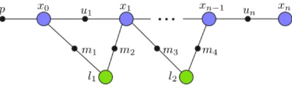
Long-term navigation necessitates the ability to re-recognize features and consequently close loops. We propose to bound the localization and mapping error by integrating VIO with high-level landmark observations using incremen-tal smoothing and mapping (iSAM) [20], [44]. In iSAM, the SLAM problem is represented is a factor graph as shown in Figure 5 where the larger colored circles are the states to be estimated and small black circles are the constraints that relate these hidden states. The VIO from Tango is used as odometry u to connect consecutive mobile robot poses xi,
and text detections are represented as measurements mj of
the text landmarks, lk. The constraints mj = {rj, θj} consist
of range a r and bearing θ. The bearing is determined based on the location of the pixel in the image at the centroid of the ER and assuming a calibrated camera. The range is
Fig. 5. Factor graph: Hidden states to be estimated are the camera poses x0..nand text landmark locations l1,l2. These states are connected through
prior p, odometry u1:nand landmark measurements m1..4.
determined by looking up the range value in the co-registered depth map at the corresponding pixel.
Under mild assumptions (such as additive Gaussian mea-surement error), the factor graph can be reduced to a nonlin-ear least squares problem which can be incrementally solved in real-time as new measurements are added [20].
V. RESULTS
We use the Google Tango device (first generation proto-type), shown in Figure 1, as the experimental platform for this work. All data were logged by the provided application TangoMapper. The VIO algorithm estimates the pose at 30 Hz using the wide-angle camera and IMU. A 1280x760 RGB image and a 360x180 depth image were recorded at 5 Hz. We developed a set of tools to parse the logged data into lightweight communications and marshaling (LCM) [45] messages, and the proposed algorithm runs on a separate laptop.
A. Dataset and Ground Truth
The “Four Score” dataset is designed 1) to compare April-Tags [46] and text detections, and 2) to test the integration of VIO with text as high-level landmarks.
Twenty-five words (shown in upper case) out of 30 words were selected from the Gettysburg Address by Abraham Lincoln:
FOUR SCORE AND SEVEN YEARS AGO OUR FATHERS BROUGHT FORTH on THIS CONTI-NENT a NEW NATION, CONCEIVED in LIBERTY, and DEDICATED to THE PROPOSITION THAT ALL MEN ARE CREATED EQUAL.
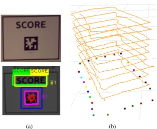
We paired each word with an AprilTag on our experimen-tal signage. The stroke width of the text is roughly the same as the grid size of an AprilTag for compatible comparisons. A ground truth rectangle is obtained from the relative real-world position to an AprilTag detection. An example is shown in Figure 6(a).
The signs were spaced roughly 1-2 meters apart. The experimenter held the Tango device and aimed the camera at each sign at various viewing angles and walked at different speeds in each pass 1. As shown in 6(b), there are nine
traverses around the loop resulting in about 3,293 RGB frames over a period of about 11 minutes. The total number of AprilTag detections is 1,286. We expect an end-to-end text spotting system to detect and decode a candidate rectangle as one of the lexicon words correctly when the paired AprilTag is detected.
B. Refining Region Proposals
The key to speed-up text spotting is to refine region proposals in an efficient manner. Table I demonstrates the numbers reduced by the proposed methods and the running time of each stage. All were implemented in C++ and
(a) (b)
Fig. 6. Text spotting and ground truth using AprilTags: (a) Top: an example sign used in the experiment. Bottom: a candidate decoded as a target in the lexicon is shown in yellow rectangles, and blue otherwise. Pink: AprilTag detection with center and id number shown in red; green: ground truth text location acquired using AprilTags the relative 3D position to the AprilTag detection; yellow: detected target text location. (b) There are nine traverses around the loop where time is shown on the z-axis. The colored markers are the estimated text locations at the end of the experiment.
OpenCV, and ran on a standard laptop computer without using GPU acceleration. The results indicate that junction features can reduce the number of region proposals of words from 779,500 to 54 in only around 100 ms, and scene priors reduce the number of ERs from 45 to 6 only with the computational cost of surface normal estimation and filtering (12 ms).
C. Retaining High Recall of Detection
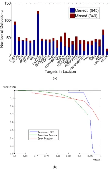
In addition to reduce the number of region proposals, the region proposals should have high recall. The sliding window approach we report that the 945 region proposals have at least 50% overlap with the 1,286 ground truth rectangles (recall rate is 0.73). The correct and missed detections for each lexicon word are shown in Figure 7(a).
TABLE I
RUNNINGTIME(MS)OFEACHPROCESSINGSTAGE,ANDAVERAGE NUMBERS OF FEATURES/REGION PROPOSALS. DECODING TIME IS IN PROPORTIONAL TO THE NUMBER OF REGION PROPOSALS(3.5MS PER
REGION USINGTESSERACTOCRENGINE).
Time (ms) Num.
Junction Features 779,500 windows Feature Extraction 4 190 FAST pts Junction Feature Encoding 75 13,383 pixels
421 junctions Region Proposal Generation 24 54 regions ERs and Scene Priors
Feature Extraction 143 45 ERs Surface Normal Estimation 11
Scene Prior Filtering <1 6 ERs Region Proposal Generation <1 3.60 regions
D. Obtaining High Precision of Decoding
In the decoding stage, we aim at high precision p at the cost of some tolerable missed detections in order to minimize false positives that will degrade the performance of the SLAM system. We compare our method with two from the literature: (i) Tesseract OCR [43] and (ii) deep features [18]. The results are shown in Figure 7-(b) and indicate that the proposed method is comparable to the other two approaches for images in frontal view.
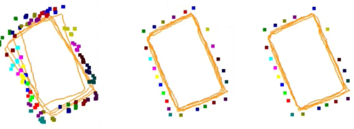
E. Text Spotting to Support Navigation
We show the trajectory and feature location estimates for three cases in Figure 8. On the left is the case of VIO alone. The sign locations drift on each pass. In the middle, we show the trajectory and feature location estimates using the AprilTag detections. On the right side is the trajectory and sign estimates using text as high-level features.
Figure 9 shows the error for both the SLAM with text case and the VIO alone case along with the uncertainty bounds calculated as the trace of the covariance matrix. The ground truth in this case is taken to be the AprilTag trajectory. For the SLAM with text case, we can see that the uncertainty in the estimate is bounded as a result of loop closure and the error and uncertainty are periodic with the size of the loop in the trajectory. In the VIO case, both the error and uncertainty grow without bound.
We also evaluated the method using the metric proposed in [47], which is designed to compare the relative energy on each link rather than the total error in the global frame. This involves calculating the relative transformation between poses in the graph δij and comparing to ground truth. In
this case we choose the poses to be used for comparison as subsequent poses:
δttext= xtextt+1 xtext t δV IOt = xV IOt+1 xV IO t δ∗t = x∗t+1 x∗t εtext= T −1 X t=0 (δttext δt∗)2 εV IO= T −1 X t=0 (δtV IO δ∗ t) 2 (1)
where xtextt , xV IOt , and x∗t are the poses of the text with
SLAM, VIO alone, and AprilTags with SLAM trajectories. The results are εtext = 21.6875 and εV IO = 25.3011
showing a higher relative error according to the metric in [47].
F. SLAM to Support Text Spotting
The SLAM has also enhanced text spotting by location priors. The pose estimation landmark estimates from SLAM act as a verification for loop closures. For a revisited text region, SLAM further verifies the detection confidence be-tween this upcoming detection and existing landmarks in iSAM, resulting in higher accuracy. In the experiment, this location prior rejects all 4 false-positives.
Fig. 8. SLAM results: The orange lines are the trajectory estimates for each of three cases: Left: VIO only. Middle: SLAM with AprilTag detections. Right: SLAM with text as high-level landmarks. Using text as landmarks notably increases the accuracy of the trajectory estimates.
VI. CONCLUSIONS
In this work we propose an integrated SLAM and text spotting system that highlights the complementary nature of these two tasks. Previous approaches to environmental text spotting are generally too slow for real-time operation. To overcome this, we propose a new junction feature that is fast and accurate for representing text. We test the performance of our system on a dataset gathered with a Google Tango and compare the performance of the text detection system against a fiducial tag system (AprilTags) as well as state-of-the-art text spotting algorithms which are much slower. The result is that our proposed method is able to balance the performance for recognizing text with the real-time requirements of SLAM, and the performance for both tasks is improved.
One important application for such a system would be as an aid to the visually impaired. Text occurs commonly in human environments, and thus is a good landmark to use for SLAM. Moreover, text can help provide robots with a higher level semantic understanding of the world necessary for more complex tasks.
REFERENCES
[1] H. Durrant-Whyte and T. Bailey, “Simultaneous localization and mapping: part I,” Robotics & Automation Magazine, IEEE, vol. 13, no. 2, pp. 99–110, 2006.
[2] K. Wang and S. Belongie, “Word spotting in the wild,” in Eur. Conf. on Computer Vision (ECCV), 2010.
[3] K. Wang, B. Babenko, and S. Belongie, “End-to-end scene text recognition,” in Intl. Conf. on Computer Vision (ICCV), 2011. [4] R. Minetto, N. Thome, M. Cord, J. Stolfi, F. Precioso, J. Guyomard,
and N. J. Leite, “Text detection and recognition in urban scenes,” in Computer Vision Workshops (ICCV Workshops), 2011 IEEE Interna-tional Conference on. IEEE, 2011, pp. 227–234.
[5] L. Neumann and J. Matas, “Real-time scene text localization and recognition,” in Proc. IEEE Int. Conf. Computer Vision and Pattern Recognition (CVPR), 2012.
[6] ——, “A method for text localization and recognition in real-world images,” in Asian Conf. on Computer Vision (ACCV), 2004, pp. 770– 783.
[7] ——, “Text localization in real-world images using efficiently pruned exhaustive search,” in Proc. of the Intl. Conf. on Document Analysis and Recognition (ICDAR), 2011, pp. 687–691.
[8] L. Gomez and D. Karatzas, “Multi-script text extraction from natural scenes,” in Document Analysis and Recognition (ICDAR), 2013 12th International Conference on. IEEE, 2013, pp. 467–471.
[9] C. Yi and Y. Tian, “Assistive text reading from complex background for blind persons,” in Proc. of Camera-based Document Analysis and Recognition (CBDAR), 2011, pp. 15–28.
[10] C.-Y. Lee, A. Bhardwaj, W. Di, V. Jagadeesh, and R. Piramuthu, “Region-based discriminative feature pooling for scene text recogni-tion,” 2014.
[11] C. Yao, X. Bai, B. Shi, and W. Liu, “Strokelets: A learned multi-scale representation for scene text recognition,” in Proc. IEEE Int. Conf. Computer Vision and Pattern Recognition (CVPR), 2014.
[12] A. Bissacco, M. Cummins, Y. Netzer, and H. Neven, “PhotoOCR: Reading text in uncontrolled conditions,” in Computer Vision (ICCV), 2013 IEEE International Conference on. IEEE, 2013, pp. 785–792. [13] H.-C. Wang, Y. Linda, M. Fallon, and S. Teller, “Spatially prioritized and persistent text detection and decoding,” in Proc. of Camera-based Document Analysis and Recognition (CBDAR), 2013.
[14] C. Case, A. C. B. Suresh, and A. Y. Ng, “Autonomous sign reading for semantic mapping,” in IEEE Intl. Conf. on Robotics and Automation (ICRA), 2011, pp. 3297–3303.
[15] M. Kaess, H. Johannsson, R. Roberts, V. Ila, J. J. Leonard, and F. Dellaert, “iSAM2: Incremental smoothing and mapping using the Bayes tree,” The International Journal of Robotics Research, vol. 31, no. 2, pp. 216–235, 2012.
[16] A. Coates, B. Carpenter, C. Case, S. Satheesh, B. Suresh, T. Wang, D. J. Wu, and A. Y. Ng, “Text detection and character recognition in scene images with unsupervised feature learning,” in Document Analysis and Recognition (ICDAR), 2011 International Conference on. IEEE, 2011, pp. 440–445.
[17] T. Wang, D. J. Wu, A. Coates, and A. Y. Ng, “End-to-end text recog-nition with convolutional neural networks,” in Pattern Recogrecog-nition (ICPR), 2012 21st International Conference on. IEEE, 2012, pp. 3304–3308.
[18] M. Jaderberg, A. Vedaldi, and A. Zisserman, “Deep features for text spotting,” in Eur. Conf. on Computer Vision (ECCV), 2014. [19] F. Dellaert and M. Kaess, “Square root SAM: Simultaneous location
and mapping via square root information smoothing,” Int. J. of Robotics Research, vol. 25, no. 12, pp. 1181–1203, 2006.
[20] M. Kaess, A. Ranganathan, and F. Dellaert, “iSAM: Incremental smoothing and mapping,” IEEE Trans. Robotics, vol. 24, no. 6, pp. 1365–1378, Dec. 2008.
[21] C. Harris and M. Stephens, “A combined corner and edge detector.” in Alvey vision conference, vol. 15. Manchester, UK, 1988, p. 50. [22] X. Zhao, K.-H. Lin, Y. Fu, Y. Hu, Y. Liu, and T. S. Huang, “Text from
corners: a novel approach to detect text and caption in videos,” Image Processing, IEEE Transactions on, vol. 20, no. 3, pp. 790–799, 2011. [23] N. Dalal and B. Triggs, “Histograms of oriented gradients for human detection,” in Computer Vision and Pattern Recognition, 2005. CVPR 2005. IEEE Computer Society Conference on, vol. 1. IEEE, 2005, pp. 886–893.
[24] L. Neumann and J. Matas, “Scene text localization and recognition with oriented stroke detection.” ICCV, 2013.
(a)
(b)
Fig. 7. Text spotting evaluation: (a) Number of correct and missed text detections. (b) Precision/recall curve of a candidate being decoded as one of lexicon words for frontal view.
[25] W. Huang, Z. Lin, J. Yang, and J. Wang, “Text localization in natural images using stroke feature transform and text covariance descriptors,” in Proc. IEEE Int. Conf. Comp. Vis, 2013, pp. 1241–1248.
[26] B. Epshtein, E. Ofek, and Y. Wexler, “Detecting text in natural scenes with stroke width transform,” in Proc. IEEE Int. Conf. Computer Vision and Pattern Recognition (CVPR), 2010, pp. 2963–2970.
[27] J. J. Lim, C. L. Zitnick, and P. Doll´ar, “Sketch tokens: A learned mid-level representation for contour and object detection,” in Computer Vision and Pattern Recognition (CVPR), 2013 IEEE Conference on. IEEE, 2013, pp. 3158–3165.
[28] C. Yi, Y. Tian et al., “Text extraction from scene images by character appearance and structure modeling,” Computer Vision and Image Understanding, vol. 117, no. 2, pp. 182–194, 2013.
[29] M. Jaderberg, K. Simonyan, A. Vedaldi, and A. Zisserman, “Synthetic data and artificial neural networks for natural scene text recognition,” in Workshop on Deep Learning, NIPS, 2014.
[30] I. Posner, P. Corke, and P. Newman, “Using text-spotting to query the world,” in IEEE/RSJ Intl. Conf. on Intelligent Robots and Systems (IROS), 2010, pp. 3181–3186.
[31] C. Case, B. Suresh, A. Coates, and A. Y. Ng, “Autonomous sign reading for semantic mapping,” in Robotics and Automation (ICRA), 2011 IEEE International Conference on. IEEE, 2011, pp. 3297–3303. [32] J. G. Rogers, A. J. Trevor, C. Nieto-Granda, and H. I. Christensen, “Simultaneous localization and mapping with learned object recogni-tion and semantic data associarecogni-tion,” in Intelligent Robots and Systems (IROS), 2011 IEEE/RSJ International Conference on. IEEE, 2011, pp. 1264–1270.
[33] R. Smith, “An overview of the tesseract OCR engine,” in Proc. of the
Fig. 9. SLAM with Text vs VIO: The red line shows the absolute error between the text with SLAM and ground truth (AprilTags with SLAM). The pink shaded region shows the 3σ bound as the sum of the trace of the covariance at each timestep. The blue line and shaded area show the corresponding plots for the VIO only case.
Intl. Conf. on Document Analysis and Recognition (ICDAR), 2007, pp. 629–633.
[34] J. Samarabandu and X. Liu, “An edge-based text region extraction algorithm for indoor mobile robot navigation,” International Journal of Signal Processing, vol. 3, no. 4, pp. 273–280, 2006.
[35] T. Ojala, M. Pietikainen, and T. Maenpaa, “Multiresolution gray-scale and rotation invariant texture classification with local binary patterns,” Pattern Analysis and Machine Intelligence, IEEE Transactions on, vol. 24, no. 7, pp. 971–987, 2002.
[36] S. Belongie, J. Malik, and J. Puzicha, “Shape matching and object recognition using shape contexts,” Pattern Analysis and Machine Intelligence, IEEE Transactions on, vol. 24, no. 4, pp. 509–522, 2002. [37] E. Shechtman and M. Irani, “Matching local self-similarities across images and videos,” in Computer Vision and Pattern Recognition, 2007. CVPR’07. IEEE Conference on. IEEE, 2007, pp. 1–8. [38] D. G. Lowe, “Distinctive image features from scale-invariant
key-points,” International journal of computer vision, vol. 60, no. 2, pp. 91–110, 2004.
[39] S. M. Smith and J. M. Brady, “Susan—a new approach to low level image processing,” International journal of computer vision, vol. 23, no. 1, pp. 45–78, 1997.
[40] E. Rosten and T. Drummond, “Machine learning for high-speed corner detection,” in Eur. Conf. on Computer Vision (ECCV), 2006, pp. 430– 443.
[41] S. Lucas, “Icdar 2005 text locating competition results,” in Proc. of the Intl. Conf. on Document Analysis and Recognition (ICDAR), 2005, pp. 80–84 Vol. 1.
[42] R. B. Rusu and S. Cousins, “3D is here: Point cloud library (PCL),” in Robotics and Automation (ICRA), 2011 IEEE International Conference on. IEEE, 2011, pp. 1–4.
[43] R. Smith, “History of the Tesseract OCR engine: what worked and what didn’t,” in Proc. of SPIE Document Recognition and Retrieval, 2013.
[44] M. Kaess, H. Johannsson, R. Roberts, V. Ila, J. Leonard, and F. Dellaert, “iSAM2: Incremental smoothing and mapping with fluid relinearization and incremental variable reordering,” in IEEE Intl. Conf. on Robotics and Automation (ICRA), Shanghai, China, May 2011, pp. 3281–3288.
[45] A. Huang, E. Olson, and D. Moore, “LCM: Lightweight communica-tions and marshalling,” in IEEE/RSJ Intl. Conf. on Intelligent Robots and Systems (IROS), Taipei, Taiwan, Oct. 2010.
[46] E. Olson, “Apriltag: A robust and flexible visual fiducial system,” in Robotics and Automation (ICRA), 2011 IEEE International Conference on. IEEE, 2011, pp. 3400–3407.
[47] W. Burgard, C. Stachniss, G. Grisetti, B. Steder, R. Kummerle, C. Dornhege, M. Ruhnke, A. Kleiner, and J. D. Tard´os, “A comparison of SLAM algorithms based on a graph of relations,” in Intelligent Robots and Systems, 2009. IROS 2009. IEEE/RSJ International Con-ference on. IEEE, 2009, pp. 2089–2095.