Design Ice Pressure-Area Relationships: Molikpaq Data

Publisher’s version / Version de l'éditeur:

PERD/CHC Report 14-121, 2005-12

READ THESE TERMS AND CONDITIONS CAREFULLY BEFORE USING THIS WEBSITE. https://nrc-publications.canada.ca/eng/copyright

Vous avez des questions? Nous pouvons vous aider. Pour communiquer directement avec un auteur, consultez la

première page de la revue dans laquelle son article a été publié afin de trouver ses coordonnées. Si vous n’arrivez pas à les repérer, communiquez avec nous à PublicationsArchive-ArchivesPublications@nrc-cnrc.gc.ca.

Questions? Contact the NRC Publications Archive team at

PublicationsArchive-ArchivesPublications@nrc-cnrc.gc.ca. If you wish to email the authors directly, please see the first page of the publication for their contact information.

NRC Publications Archive

Archives des publications du CNRC

For the publisher’s version, please access the DOI link below./ Pour consulter la version de l’éditeur, utilisez le lien DOI ci-dessous.

https://doi.org/10.4224/12340981

Access and use of this website and the material on it are subject to the Terms and Conditions set forth at Design Ice Pressure-Area Relationships: Molikpaq Data

Jordaan, I.; Li, Chun; Mackey, T.; Nobahar, A.; Bruce, Jonathon

https://publications-cnrc.canada.ca/fra/droits

L’accès à ce site Web et l’utilisation de son contenu sont assujettis aux conditions présentées dans le site LISEZ CES CONDITIONS ATTENTIVEMENT AVANT D’UTILISER CE SITE WEB.

NRC Publications Record / Notice d'Archives des publications de CNRC: https://nrc-publications.canada.ca/eng/view/object/?id=7ae68ec8-d3a7-47c8-b1c8-46ee4da67df6 https://publications-cnrc.canada.ca/fra/voir/objet/?id=7ae68ec8-d3a7-47c8-b1c8-46ee4da67df6

Design Ice Pressure-Area Relationships

Design Ice Pressure-Area Relationships; Molikpaq Data

PERD/CHC Report 14-121

December 2005 Prepared for:

National Research Council Canada Canadian Hydraulics Centre

and

Panel on Energy Research and Development (PERD)

Prepared by:

Memorial University of Newfoundland Ian Jordaan

Chuanke Li Thomas Mackey

Arash Nobahar Jonathon Bruce

SUMMARY

For the design of offshore structures, global loads are an important factor to be considered in ensuring the overall integrity of the structure. The scale effect whereby average global pressures are much smaller than those measured on small areas is an aspect in the determination of global loads. There are significant probabilistic issues in the relationship between small and large areas that are related to the scale effect. A study of the mechanics of ice failure, for interactions where crushing is dominant, shows that the failure occurs in localized zones, termed high pressure zones, through which most of

the load is transmitted. These zones are of the order of 0.1 m2, and occur roughly at an

areal density of 1m-2. Fractures play an important part in the process, contributing areas

of low or zero stress.

Full scale data are most important in understanding and in determining design loads. In the report, the Molikpaq data are analyzed, in particular those from the Medof panels. Since these panels cover an area less than 10% of the area of a face during interaction with ice, the local effects can dominate the measurements of loads, and extrapolation to the entire face must be done with care. In the past, conservative approaches have been taken. Here, a preliminary analysis of these results has been conducted, based on a modification of the method of Timco and others. First, the data shows that Medof panel forces correlate on adjacent panels while they do not correlate on detached panels. A correlation coefficient of about 0.6 to 0.8 has been estimated for adjacent panels, with little or no correlation for distant ones.

The analysis is based on the observation that the correlation coefficient between adjacent Medof panels is about 0.6 to 0.8 and close to zero for distant panels. A Markov approach has been taken, using where appropriate a first-order autoregressive model in space. Three models have been used, in all cases reducing the average column variance over measured panels to that of an individual column, and then to that of the entire loaded face (the global pressure). In the first of the three methods (Method 1), the Medof panels were considered to be a group of adjacent panels (columns). In the second and third methods, independent groups of pairs of panels (columns) were considered. The members of each pair were combined using autoregressive methods (Method 2) and using the correlation coefficients (Method 3). Where there are more than four pairs of panels, a similar methodology was used, but considering a different number of columns.

When these models are applied, the global ice pressure on an area 90 m wide has a mean of 0.23 MPa and standard deviation of 0.042 to 0.054 MPa for a correlation coefficient of

0.6, and 0.044 to 0.065 MPa for a correlation coefficient of 0.8. This can be compared to a value of 0.040 MPa if independence between columns is assumed. It is considered that Method 3 presents the best analysis at present yet further investigation is warranted. The results show that the global load estimates taking into account probabilistic averaging are significantly lower than when estimated by linear extrapolation from the Medof panels. Since strain gauge data are also representative of a local areas, a similar approach should be taken when using these data. It is concluded that an exhaustive and integrated analysis of all Molikpaq data would be of great usefulness and interest for the ice community.

TABLE OF CONTENTS SUMMARY... I 1 INTRODUCTION ... 1 2 BACKGROUND TO MOLIKPAQ... 2 2.1 General... 2 2.2 Load Monitoring ... 3 2.2.1 Medof panels... 6 2.2.2 Strain Gauges ... 7 2.2.3 Extensometers ... 7 2.2.4 Accelerometers ... 8

3 PAST WORK USING MOLIKPAQ DATA ... 10

3.1 Load Calculations Based on Molikpaq Ice Load Instrumentation... 10

3.2 Load Estimates Based on Foundation Displacement... 14

3.3 General Comments and Points of Interest ... 16

4 ICE LOADING AS A RANDOM PROCESS... 18

4.1 Relevant Ice Mechanics ... 18

4.2 Ice Loads and Probabilistic Methodology ... 19

4.3 Determination of Global Load Paramters – Molikpaq, Amauligak I-65 ... 21

4.3.1 Introduction... 21

4.3.2 Methodology ... 22

4.3.3 Illustrative Example ... 24

4.3.3.1 Convert the data into a useable format. ... 25

4.3.3.2 Produce an event average pressure data series ... 25

4.3.3.3 Trim the event average pressure curve and calculate the mean and standard distribution... 26

4.3.3.4 Calculate the standard deviation for individual columns from groups of contiguous panels and for global pressure for each event—Method 1... 27

4.3.3.5 Calculate the standard deviation for an individual column from groups of two adjacent columns and for global pressure for each event—Method 2... 28

4.3.3.6 Calculate the standard deviation for a group of two adjacent columns using a linear function of random quantities and for global pressure for each event— Method 3 29 5 CONCLUSIONS AND DISCUSSION ... 38

5.1 Observations and Conclusions... 38

5.2 Discussion: Nonsimultaneous Failure, Probabilistic Averaging and Phase-Lock ... 39

6 REFERENCES ... 40

APPENDIX A: EVENT GRAPHS... A APPNDIX B: MEDOF PANEL DESCRIPTIONS ... BB LIST OF TABLES Table 2-1 Design Load used for the Molikpaq (from Rogers et al., 1998). Centre column amended to “tons” from “tonnes”. ... 3

Table 2-2: An Overview of the Molikpaq instrumentation system while at the Tarsiut P-45 site. (Jefferies and Wright, 1988)... 9

Table 3-1: Significant loading events as reported by Jefferies and Wright (1988) ... 10

Table 3-2: Table of ice loading events from Sanderson (1988)... 13

Table 3-3 Load estimate comparison... 17

Table 4-1: The mean and standard deviation of events calculated with modified line load method. “Local” standard deviation refers to that of the Mean Average Pressure on the Columns. ... 31

Table 4-2 Table showing the results and methodology for calculating a new standard deviation for the individual column and global standard deviation based on ρ = 0.6 and c = 0.82. Method 1. ... 32

Table 4-3 Table showing the results methodology for calculating a new standard deviation for the individual column and global standard deviation based on ρ = 0.8 and c = 1.4. Method 1. ... 33

Table 4-4 Table showing the results methodology for calculating a new standard deviation for two adjacent columns and the global standard deviation based on an autoregressive model with ρ = 0.6 and c = 0.82. Method 2. ... 34

Table 4-5 Table showing the results methodology for calculating a new standard deviation for two adjacent columns and the global standard deviation based on an autoregressive model with ρ = 0.8 and c = 1.4. Method 2. ... 35

Table 4-6 Table showing the results methodology for calculating a new standard deviation for two adjacent columns using linear functions of random quantities with ρ = 0.6 and the global standard deviation based on an auto regressive model with c = 0.82. Method 3. ... 36

Table 4-7 Table showing the results methodology for calculating a new standard deviation for two adjacent columns using linear functions of random quantities and the global standard deviation based on an auto regressive model with ρ= 0.8 and c = 1.4. Method 3. ... 37

LIST OF FIGURES

Figure 2-1 Ice failure modes during the 1985/86 season. Note that crushing was observed to take place only a small portion of the time ... 4 Figure 2-2 Schematic illustration of the Molikpaq showing the structural characteristics

and load monitoring instrument placement. (from Jefferies and Wright, 1988) ... 5 Figure 2-3: Medof panel array numbering with letters representing columns... 7 Figure 4-1: Schematic representation of Ice structure interaction and the formation of

High Pressure Zones (from Jordaan, 2001) ... 18 Figure 4-2 Pressure trace simulation for 20 seconds. The six green lines are pressure

traces of six individual Medof panels. The thick blue line is the average of the six panels and the thick red line is the average pressure over the whole structure. ... 20 Figure 4-3 Peak pressure for different loading periods from 1 minute to 1 hour. ... 21 Figure 4-4 Loaded Medof panels used in analysis fast file f603081731, note that 8

columns (vertical cross sections), and 14 panels are loaded... 24 Figure 4-5 Medof data, fast file f603081731; this shows individual load data for 14

loaded panels after zeroing. ... 25 Figure 4-6 : Average pressure graphs for fast file f603081731 ... 26

1 INTRODUCTION

The calculation of global loads on structures is important so to maintain the integrity of the structure during its service life. These loads are estimated using probabilistic methods (Jordaan, 2005). Because of the complex nature of the failure process, it is important to use to the fullest extent possible, full scale load measurements.

The Molikpaq provides a unique opportunity to study large scale ice loading on offshore structures. During its deployments in the Canadian Beauforte Sea during the 1980’s, (for a full description of the deployments see Rogers et al., 1998) the Molikpaq experienced multiple interactions with many types of ice. The Molikpaq is said to have behaved well during most of the interactions. On several occasions the structure experienced significant dynamic loading. In one instance (most notably the ice loading event of April 12, 1986), there was partial failure of the sand core (Jefferies and Wright, 1988).

Instrumentation data, visual reports, and interaction logs are available for a large number of the ice loading events, and can be used to provide valuable insight and understanding into full scale ice-structure loading and interaction behavior. It is not a trivial exercise to interpret this information and determine the ice loads. This complexity has lead to

differing opinions on how the available data should be treated and consequently, what the magnitudes of the loads experienced by the Molikpaq were.

This report aims to demonstrate a new probabilistic method of interpreting the loading data available from the Medof panels. These panels are relatively small, and cover about 8% of a particular face of the structure. Pressures on small areas are known to be much more variable than those on bigger areas. The question arises as to how measurements from these small areas should be extrapolated to capture the variation on the larger faces of the structure. The new method differs from past load estimations based on the Medof data by providing a global pressure analysis that recognizes the limited spatial coverage of the panels, and thereby removes some of the conservatism in present methodology.

2 BACKGROUND TO MOLIKPAQ 2.1 General

During the 1970s and 1980s, the Canadian Beaufort Sea was an area of interest for hydrocarbon exploration. Companies such as Gulf Canada Resources Ltd., ESSO Resources Canada Ltd. and Dome Petroleum were active. All three companies used artificial island and caisson technology for exploration in order to provide ice-resistant platforms suitable for extended winter season drilling.

The Molikpaq concept, developed by Gulf Canada Resources Ltd.,extended previous

island and caisson experience since it was designed as a deep draft caisson capable of operating in water depth range of 20 m to 40 m (considered significantly deep at the time). A consequence of this deep caisson design was that the protective rubble formation found around caissons and islands operating in shallower waters was not expected to form, and the caisson was expected to interact directly with moving winter pack ice. Conceptual design of the structure began in late 1980 with fabrication commencing in late 1981 (at the AICHI yard of Isikawajima-Harima Heavy Industries in Nagoya, Japan) and was completed in the spring of 1984. The Molikpaq is essentially a continuous steel annulus, octagonal in plan, supporting a deck, which carries the entire drilling and “topsides” facilities. It has a height from base to deck level of 29 m, while plan dimensions range from 111 m at the base to 86.6 m at deck level. An ice and wave deflector is mounted around the perimeter of the deck.

The Molikpaq was designed so that it could be set down directly on the seabed or on a prepared berm pre-built at the site to suit local bathymetry and subsurface soil conditions. The core space was then in-filled with sand fill material. The geotechnical stability was designed to be achieved from:

1. The friction (soil/steel) generated by the weight of the steel caisson on the supporting berm.

2. The mass of the sand-fill placed within the core of the caisson, in particular the frictional resistance generated by its weight on the supporting berm.

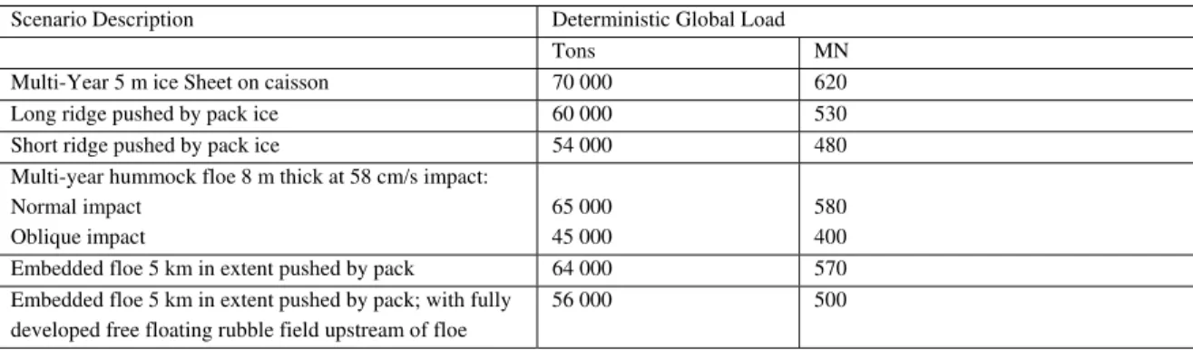
The Molikpaq was originally designed (Golder, 1981) to achieve an ultimate horizontal sliding resistance to ice loading of 890 MN; this was later revised to a global load of 620 MN (Rogers et al., 1998) as shown in Table 2-1. Sanderson (1988) and Rogers et al.

(1998) note that the estimated design load of the Molikpaq was then later reduced to 500 MN as data from the Hans Island experiments became available. These is lower than initial estimates of global ice loads. Sanderson notes that with the 1.4 factor of safety used in design, the structure was still thought to be able to withstand loads upwards of 700 MN.

Table 2-1 Design Load used for the Molikpaq (from Rogers et al., 1998). Centre column amended to “tons” from “tonnes”.

Scenario Description Deterministic Global Load

Tons MN

Multi-Year 5 m ice Sheet on caisson 70 000 620

Long ridge pushed by pack ice 60 000 530

Short ridge pushed by pack ice 54 000 480

Multi-year hummock floe 8 m thick at 58 cm/s impact: Normal impact Oblique impact 65 000 45 000 580 400

Embedded floe 5 km in extent pushed by pack 64 000 570

Embedded floe 5 km in extent pushed by pack; with fully developed free floating rubble field upstream of floe

56 000 500

2.2 Load Monitoring

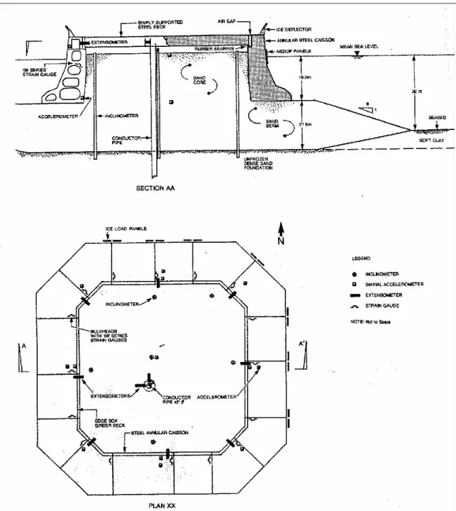
The Molikpaq was considered to present an excellent opportunity to study ice loading. It operated in many ice conditions. Figure 2-1 shows results of observations for the 1985-6 season. It was heavily instrumented to monitor ice loads (Figure 2-2). The following section is based upon Rogers et al. (1998) and provides a good description of the ice monitoring instrumentation available on the Molikpaq. It should be noted that discrepancies exist within the literature as to the capabilities of the various sensors.

Figure 2-1 Ice failure modes during the 1985/86 season. Note that crushing was observed to take place only a small portion of the time

For the purposes of monitoring ice loading, instrumentation was as follows: 1. Direct measurement of local ice load (Medof panels);

2. Indirect measurement of ice load (bulkhead strain gauges);

3. Indirect measurement of face load inferred from caisson ovalling, or caisson movement relative to the centre guide pipe (extensometers);

Figure 2-2 Schematic illustration of the Molikpaq showing the structural characteristics and load monitoring instrument placement. (from Jefferies and Wright, 1988)

The electronic monitoring used a Hewlett Packard 9920 microcomputer in tandem with two Hewlett Packard 6944 multi-programmers. Scan data was initially stored onto 15 MByte hard discs, which were backed up onto DC600 tape cartridges. The hard discs configured in 1984 were the largest available at the time for microcomputer based systems and it was this maximum stored data limit that determined how the data acquisition was configured. Three modes of data acquisition were used to obtain the required information while remaining within the limit of the system. These modes were:

1. Slow scanning (5 minute average, maximum and minimum on all channels); 2. Fast scan rate (1 to 10 Hertz scanning of all channels);

3. Burst scan rate (50 or 75 Hertz scanning of a key sub-set of channels).

The platform response was the principal determinant of the mode used. Slow scanning was used for normal operations. Accelerometer and extensometer output were used to trigger a fast or burst scan rate if the thresholds input by the monitoring team were exceeded. Mode control was carried out by the HP 9920 computer and a rolling buffer scheme was used so that a few seconds of data leading to the trigger event were recorded as well as the post trigger period. This faster scan data was designed to document the dynamic response of the Molikpaq. The burst file was limited to a 90 second block, and allowed a “snapshot” of a particularly strong sequence of dynamic response.

Furthermore, if the dynamic response became larger during the event then a quasi-continuous record (to the limit of the storage) was obtained. The fast scan ran in parallel with the burst scanning. As the fast scan was typically 1/50th of the rate used in the burst system, much longer scan durations were possible, even though more transducer channels were being recorded. The limitation of the fast scan system was its inability to resolve the nature of the platform dynamics. It did, however, capture information related to the quasi-static loading.

2.2.1 Medof panels

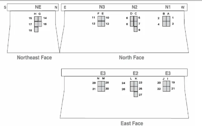
Thirty one Medof panels, 1.135 m wide and 2.715 m high, with a capacity of 20 MN were installed on the north, northeast and east face of the caisson (Figure 2-3). The panels were arranged in seven clusters of four or five panels. The panels are configured so that they measure the total force acting on the plate, regardless of how it is distributed or where it acts (Metge et al., 1983). Slightly more than 10% of the length of each the north and east faces are covered with panels. The areal coverage could be less.

Figure 2-3: Medof panel array numbering with letters representing columns

2.2.2 Strain Gauges

Over 200 strain gauges were installed during Molikpaq construction on the north, northeast, and east segments of the caisson, covering locations on ribs for the ice and sand faces, the base plate, and on the main and intermediate bulkheads. Experience with the response of these strain gauges showed that those referenced as the ‘09 series’ had the best sensitivity and linearity for the load measurement of ice up to 5 meters thick (Rogers et al., 1998). Additional ‘09 series’ gauges were therefore installed on the Molikpaq in April 1986 to give coverage at sixteen main bulkhead locations around the structure.

2.2.3 Extensometers

As ice loads are applied to the Molikpaq the annular caisson deforms in an oval manner, this ovalling was sensed using pairs of extensometers. Eight rod extensometers are mounted at deck level at the midpoint of each caisson side to monitor movement between the caisson annulus and the box girder deck. Two additional extensometers were mounted in the drill collar of the box girder deck to monitor movement of the deck relative to the conductor casing, to provide a measure of absolute caisson deformation.

Rogers et al. (1998) note that a limitation of the extensometers as a method of estimating ice loads is that, although the extensometers have excellent frequency response, the parameter being sensed (ovalling) is in fact a caisson behavior and as such is affected by caisson motion during dynamic events and by the interaction of ice on other faces of the caisson. The calibration also assumes that the sandfill stiffness does not change during the ice load event.

2.2.4 Accelerometers

Platform response to ice load was also monitored by accelerometers. Sixteen biaxial accelerometers were mounted at deck level in each of the caisson sides to measure dynamic response and overall caisson tilt. Four additional pairs of biaxial accelerometers were installed near the base of the caisson in pump or valve rooms in the centre of each long side. In the centre of the core space a triaxial and biaxial accelerometer set were located at the top of the core surface, and in a bore hole near the base of the caisson, respectively. The response data from the accelerometers were used to assess the structure and sandfill response to loading.

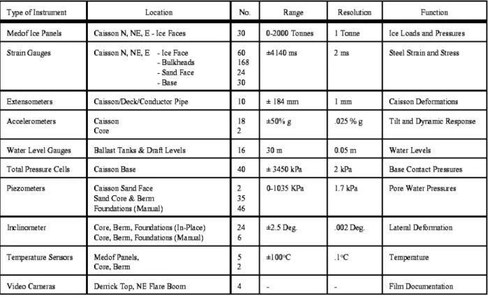
Table 2-2: An Overview of the Molikpaq instrumentation system while at the Tarsiut P-45 site. (Jefferies and Wright, 1988)

3 PAST WORK USING MOLIKPAQ DATA

3.1 Load Calculations Based on Molikpaq Ice Load Instrumentation The paper “Dynamic Response of Molikpaq to Ice Structure Interaction,” written by Jefferies and Wright (1988), is a primary work heavily referenced by others. The authors provide information on dynamic ice loading and phase lock during 1985-86. Concerning the Medof panels the authors note that although the ice load panels provide a direct measure of ice load, they have a limitation in that the response time to a step change in load is in the order of 5 to 10 seconds, rendering them inefficient for the measurement of

cyclic ice forces with fundamental frequencies in the range 0.5 to 3 Hz. Dynamic ice

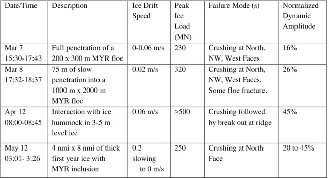
loading was measured by strain gauges. Jefferies and Wright report that a significant ice load is one greater then 100 MN, of which eighteen were recorded in first year ice and six were recorded in multi-year ice. Greater significance is placed on four events, which are said to be greater than half the design load (Table 3-1).

Table 3-1: Significant loading events as reported by Jefferies and Wright (1988)

Date/Time Description Ice Drift Speed

Peak Ice Load (MN)

Failure Mode (s) Normalized Dynamic Amplitude Mar 7 15:30-17:43 Full penetration of a 200 x 300 m MYR floe 0-0.06 m/s 230 Crushing at North, NW, West Faces 16% Mar 8 17:32-18:37 75 m of slow penetration into a 1000 m x 2000 m MYR floe 0.02 m/s 320 Crushing at North, NW, West Faces. Some floe fracture.

26%

Apr 12 08:00-08:45

Interaction with ice hummock in 3-5 m level ice

0.06 m/s >500 Crushing followed by break out at ridge

45%

May 12 03:01- 3:26

4 nmi x 8 nmi of thick first year ice with MYR inclusion 0.2 slowing to 0 m/s 250 Crushing at North Face 20 to 45%

The authors of the paper noted above suggest that the ice structure interaction leading to dynamic response is a uniform rather than a stochastic process, noting that the same peak load may not be experienced across the crushed zone; the cyclic loading of each zone nevertheless is in “phase-lock” across the entire zone of crushing.

The report “DynaMAC: Molikpaq Ice Loading Experience” by Rogers et al. (1998) relies heavily on a previous paper by Jefferies and Wright (1988), but it has expanded the scope making this a valuable source of information concerning the Molikpaq. The authors report the same loads as Jefferies and Wright (1988) noting that:

1. Load information is derived from three Medof panel groups on the north and east long faces respectively, and one Medof panel group on the northeast short face. The loads from any of these seven groups can be treated as a local load. It is the comparison of these local load synchronizations, which allow issues such as non-simultaneous or phase-locked failure to be addressed from measurements. 2. The long face of the Molikpaq at the operating waterline is approximately 60 m,

and so the coverage of the sensing groups is about 10% of the long face. Face loads are estimated by assuming that the pressures measured by each group correspond to the pressures acting over the adjacent part of the face; comparison of the synchronization between each of the three sensor groups and load variation experienced by each allow determination of the uncertainty inherent in the

calculated face load because of this assumption.

3. Temperature sensors (RTD's) are embedded into the caisson outer plate directly behind several of the panels, which allow thermal corrections to be made. 4. Thickness measurements are required to establish ice pressures. These

measurements were not usually made, and ice thickness estimates had to be determined from video and visual observations.

5. Within this paper, the authors also discuss the method by which the data was collected. Of particular note; only one set of filters was used at Tarsiut P-45 and Amauligak I-65 suggesting it also follows that the filter frequency was too high to anti-alias the fast scan signals meaning that

• fast scan data should not be analyzed with spectral methods;

• spectral analysis of burst data must allow for the excessive filtering. With regard to points 1 and 2, no evidence of statistical analysis of this effect was found by the writers of the present report in the works cited. The frequency response of the Medof panels makes analysis of synchronization difficult.

The authors of the reports cited are aware that Hewitt (1994) and Hewitt et al. (1994) are not in agreement with them (see below), and they respond with the following:

“Two comments are particularly noteworthy when considering the April 12, 1986 event. These are that:

• Only 2 of the 18 piezometers in the sand core showed liquefaction. Of the remaining 16 gauges, the majority show small to negligible pore water pressure increase. This confirms that liquefaction was localized;

• If the measured pore water pressures are used to calculate an available resistance which includes the liquefied zone, the available global resistance of the Molikpaq is still in excess of 500 MN.”

In the report “Ice Pressure Distributions from First-Year Ice Features Interacting with the Molikpaq in the Beaufort Sea”, Frederking et al. (1999) report that the Medof panels give an accurate representation of the load and that the panels are accurate up to frequencies of about 0.5 Hz. By grouping ice loads measured by the panels in various ways to allow estimates of average ice pressure as a function of area, and vertical and horizontal distributions, a methodology is derived and presented for estimating the maximum line loads These are given for a given annual exceedance probability and a given annual number of loading events. They note that the pressure calculations should be used with caution, as the actual thickness of the ice was not known. They suggest that mixed modal loading per panel was generally less than 2 MN and crushing loads were up to 3.5 MN per panel (on page 545 a load of 4MN per panel is also mentioned). This paper represents an attempt to look at how adjacent panels carried load and thus correlate loading across the structure.

Timco et al. (2005) in the paper “Multi-Year Ice Loads on the Molikpaq: May 12, 1986

Event” examine the May 12th, 1986 event, suggesting that “all of the sensors were

operating during this impact so it is possible to determine the load using each of the sensors”. The approach used to calculate loads is based on extrapolating the response measured locally to the full width of the face. It was noted that this will have some inaccuracies, but suggested it is the best approach available. They estimate peak load at 250 MN based on Medof Panels and 200 MN based on the strain gauges and suggest that the difference is a reflection of the low frequency response of the Medof panels, which begin to roll off at 1 Hz. The authors also performed a uniform deceleration analysis and calculated an average force of 26 MN, reporting that such a large difference is the result of the uniform deceleration assumption.

Timco and Johnston (2003) in the paper “Ice loads on the Molikpaq in the Canadian Beaufort Sea” state that the Medof panels provided the most useful information on ice loads. ‘‘Face’’ loads were determined from the measurement of loads on individual Medof panels. To calculate the face loads, group loads on individual Medof clusters were

first determined. To determine the load on the north face, the group load for each cluster area (i.e. N1, N2, and N3) was derived from the panel loads in each cluster. Based on visual observations, a contact factor was assigned to each of the clusters for each event. The contact factor ranged from 0 (i.e. no ice contact) to 1 (i.e. full contact). Once the contact factor had been applied, the group loads on each cluster were summed to

determine the total face load. Since the panels did not cover the whole face, a ratio of the face length to the total panel width (7.11 m) was used to factor-up (increase) the values to account for the loaded width of the structure.

The same procedure was used for the shorter northeast face by using an appropriate length scale. Global loads were determined by taking the vector sum of the individual face loads, using algebra to apportion the principal components of the loads on the short caisson faces. Loading direction was determined from the arc tangent of the two principal (N–S and E–W) load vectors. This technique resulted in a highest line load being 1.8 MN/m and highest global Pressure of 1.8 MPa.

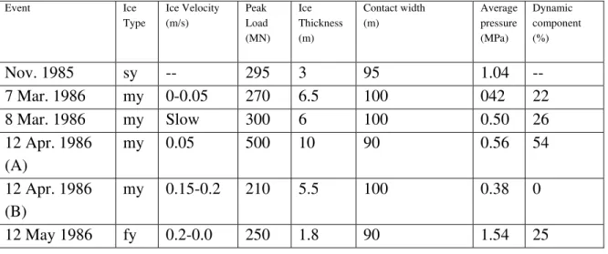
Sanderson (1988) in his book “Ice Mechanics: Risks to Offshore Structures,” estimates the ice loads using the arrays of Medof panels, describing his method as follows; “The pressures measured in each group of panels were used to evaluate the local ice pressures over vertical strips of width 1.3 m and the results for all such strips were averaged to calculate an average pressure on each face. This average pressure was then multiplied by the apparent contact area of ice with each face.” Sanderson notes that this method would likely lead to an over estimation of the load since the panels only cover approx 10 % of the structure. Sanderson provides the following table in his book addressing what he calls the “Principal ice loading events on the Molikpaq…” noting that most of the ice

thicknesses are best estimates.

Table 3-2: Table of ice loading events from Sanderson (1988) Event Ice Type Ice Velocity (m/s) Peak Load (MN) Ice Thickness (m) Contact width (m) Average pressure (MPa) Dynamic component (%) Nov. 1985 sy -- 295 3 95 1.04 -- 7 Mar. 1986 my 0-0.05 270 6.5 100 042 22 8 Mar. 1986 my Slow 300 6 100 0.50 26 12 Apr. 1986 (A) my 0.05 500 10 90 0.56 54 12 Apr. 1986 (B) my 0.15-0.2 210 5.5 100 0.38 0 12 May 1986 fy 0.2-0.0 250 1.8 90 1.54 25

3.2 Load Estimates Based on Foundation Displacement

The papers written by Hewitt et al. (1994) and Hewitt (1994) are contrary to most other papers discussing the Molikpaq experience in that they estimate the global ice load to be significantly less than most others (Jefferies and Wright, 1988; Sanderson, 1988; Rogers et al., 1998; and others).

The main objective of these works is to show that recorded foundation displacements are generally low, indicating from a geotechnical perspective, lower then expected ice loads. The authors note two problems with using Medof panels, and why they lead to

overestimation of loads.

1. The average ice pressure decreases significantly as contact width or contact area increases, due to the fact that an ice sheet does not fail simultaneously or at a uniform pressure across the entire contact face. During brittle failure of an ice sheet, high local peak pressure fluctuations are measured by the instrumentation over time and across the width of the structure. By averaging local pressures across the face of the structure, an approach that has been used in the past, one assumes that the peak pressure at each location occurred at the same time and between instrumented locations. The non-instrumented areas often account for more than 85% of the total caisson face. This type of analysis leads to an

overestimation of the global peak ice load since this load is also assumed to be as high, or last as long as the average of all the peak local ice pressures.

2. The compliance of the structure is not well understood, leaving error in the estimation of the global ice loads based on local measurements against a “vibrating” structure, the authors use the Molikpaq as an example.

The authors also note that Jeffries and Wright (1988) estimate a load “marginally in excess of the design load (500MN)” using strain gauge data (because the Medof panels could not respond to periods below 6 seconds) and that these data were calibrated using the Medof ice panels themselves (admittedly at low frequency loading). The authors then provide the following list of problems associated with this.

1. The total load was interpreted from the average of the peak load on each Medof panel, which covered only 8% of the total caisson face. The assumption that the local peak ice loads represent the total global peak ice load over the entire face of the structure leads to a large overestimation of the load.

2. During most of the calibration events, the ice thickness was not measured. 3. The Medof panels had problems as emulsification of the fluid in the panel,

shifting the baseline and creep.

4. Extensometers measure loads indirectly and measurements must be

deconvolved to remove the relative displacement between the deck and the caisson ring.

5. The Molikpaq is a compliant structure, which resulted in large

deformations and accelerations of the caisson faces due to vibrations under the largest ice loads.

6. Most of the strain gauges at the time of the important events were not functional. Analysis had to be based on only ONE strain gauge located close to a large opening (with high strain gradients) in an internal bulkhead in a complex structure.

7. The dynamic component of the strain gauge signal was assumed to be entirely attributed to the ice load.

8. Numerical models are needed to estimate load from instrumentation response and most include a realistic representation of the loose sand core. Unlike the SSDC, lateral loads on the Molikpaq are not transmitted

directly to the foundation. At high load levels, approximately 80% of the load is transmitted via the sand core. Since the sand core liquefied during the April 12 event, any correlation between strain and load would be highly non-linear.

Based on these arguments, the authors give the opinion that the global load on the Molikpaq was not easily quantifiable using the ice instrumentation available at the time of the April 12, 1986 event. They suggest a global load for this event based on

foundation displacements to be 110 MN, noting that this would be based on a single static load and the fact that the load was cyclic, and might be expected to yield a greater

cumulative effect, that in reality the load may be less than 110 MN.

Hewitt (1994) specifically deals with the April 12th 1986 event, and that the stability of

placement chosen for the sand (single point discharge near the sea surface) was the worst possible method, resulting in the loosest sand possible. Based on traditional geotechnical methods of evaluating sand densities, the core sand was loose with a relative density between 30-40 %.

Using the following geotechnical points Hewitt provides an interpretation of the global ice loads on the Molikpaq during the April 12, 1986 event:

1. The sand in the area of the loaded face settled by 1500 mm, implying extensive fluidization.

2. Pore water pressure of over 150 kPa recorded around the perimeter of the core, which corresponds to 100% of the vertical stress.

3. A deformation of 12 mm was recorded for the central casing, although the surface displacement in the direction of the load was actually zero.

4. The extensometers showed a 10 mm displacement.

5. The loaded face of the caisson settled by 35 mm which is indicative of a low-load vibration response, noting that McCreath et al. (1982) described a rising mechanism that would be associated with high loads.

The general idea is that since the sand had liquefied around the perimeter, the ultimate lateral load resistance of the structure should be estimated at 200 MN. Since the movements of the structure were small during the loading event, it is assumed that the actual peak loads were less then 200 MN (noting that application of the Hans Island multiyear ice load data set to this event indicates an upper load limit of 230 MN for 4 m thick multiyear floe). As in Hewitt et al. (1994), a maximum load of 110 MN and likely less than 100 MN is concluded.

3.3 General Comments and Points of Interest

The above summaries provide a short overview of the body of work that has been

reviewed. In general, the vast majority of the reported loads have been calculated using a method based on local means from the strain gauge and the Medof panel data. The difference in the papers often lies in the particular event that was analyzed, or in

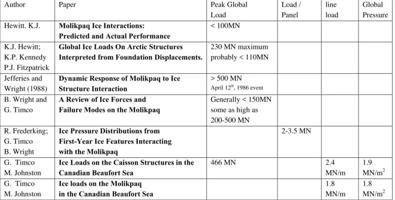
classifying the loads into categories based on ice type, mode of failure and contact width. The loads reported from a variety of sources are shown in Table 3-3 for easy comparison.

Some points of interest are

1. Discrepancies exist within the literature concerning the nature of the instrumentation, mainly the Medof panels.

2. It is noted that the method (see Sanderson and Hewitt) of averaging across the Medof panels, which cover only a portion of the structure, will lead to an overestimation. This, although noted, is not effectively dealt with in the current literature.

3. Hewitt (1994) and Hewitt et al. (1994) provide a quite different description of the consequences of the liquefaction (and the extent of liquefaction) of the sand during the April 12, 1986 than Wright and his colleagues. This results in load estimates that vary by a factor of 5.

Table 3-3 Load estimate comparison

Author Paper Peak Global

Load Load / Panel line load Global Pressure Hewitt. K.J. Molikpaq Ice Interactions:

Predicted and Actual Performance

< 100MN K.J. Hewitt;

K.P. Kennedy P.J. Fitzpatrick

Global Ice Loads On Arctic Structures Interpreted from Foundation Displacements.

230 MN maximum probably < 110MN Jefferies and

Wright (1988)

Dynamic Response of Molikpaq to Ice Structure Interaction

> 500 MN

April 12th_{, 1986 event} B. Wright and

G. Timco

A Review of Ice Forces and Failure Modes on the Molikpaq

Generally < 150MN some as high as 200-500 MN R. Frederking; G. Timco B. Wright

Ice Pressure Distributions from First-Year Ice Features Interacting with the Molikpaq

2-3.5 MN

G. Timco M. Johnston

Ice Loads on the Caisson Structures in the Canadian Beaufort Sea

466 MN 2.4 MN/m 1.9 MN/m2 G. Timco M. Johnston

Ice loads on the Molikpaq in the Canadian Beaufort Sea

1.8

MN/m

1.8 MN/m2

4 ICE LOADING AS A RANDOM PROCESS 4.1 Relevant Ice Mechanics

A study of the mechanics of ice failure (Jordaan, 2001), for interactions where crushing is dominant, shows that the failure occurs in localized zones, termed high pressure zones,

through which most of the load is transmitted. These zones are of the order of 0.1 m2, and

occur roughly at an areal density of 1 m-2. Fractures play an important part in the process,

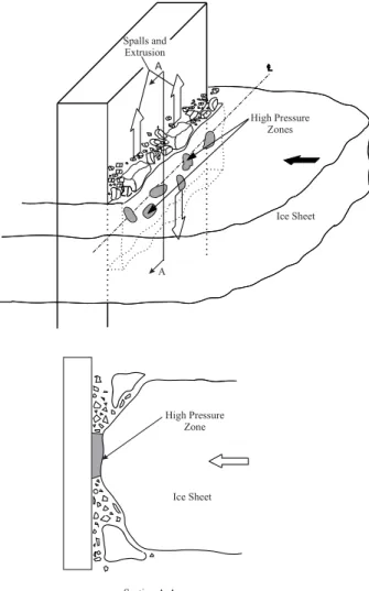
contributing areas of low or zero stress. This is well illustrated by Figure 4-1 showing that during an interaction the presence of spalling and fracture will cause some areas of the ice to experience relative unconfined conditions while other areas are highly

confined. The areas of high pressure are randomly orientated and change location as an interaction advances in time. It is proposed that this process can be modeled using probability theory.

Figure 4-1: Schematic representation of Ice structure interaction and the formation of High Pressure Zones (from Jordaan, 2001)

4.2 Ice Loads and Probabilistic Methodology

Ice load measurements on the Molikpaq, Amauligak I-65 deployment are analyzed in this study. Significant discrepancies exist within the literature regarding ice loads estimated from the Medof panels. Within this report, a practical probabilistic approach is taken in analysing the Medof panel data, that takes into account the fact that only a portion of the structure was instrumented, leading to estimates of global standard deviation appropriate for extrapolation to determine face loads. An ice-structure interaction event can be idealized as a random averaging process, and the assumption has been made that the process is stationary in order to characterize the process.

As just noted, it is assumed that the process is stationary. This assumption of stationarity is often questioned. The data has many fluctuations, due to fractures, splits, and

variations in ice thickness and other dimensions (for example). If all of these aspects were measured, for instance if local variations in ice thickness were measured, one could develop a model to account for these effects. In the context of the present observations, it is idle to state that there is a non-stationary process, since there is no basis to develop physical reasoning to explain the non-stationarity, and it cannot properly be modelled. Rather the causes of the load fluctuations are considered as background random events within a stationary process, contributing to the variance. The process is therefore treated as stationary for a given time interval.

As an illustration of our thinking, we start with the formulation of a probabilistic model. The model consists of an ice-structure interaction surface consisting of a random number of high-pressure zones with an area lost due to fracture. Using the statistics of the

formation of high pressure zones, a stochastic model of the global pressure exerted on a structure with given dimensions can be obtained. The following example is intended to demonstrate the potential of the method, and is not based on a definitive calibration of the model. It is based on the Molikpaq structure. In the simulation, for demonstration

purposes, the mean density of the high pressure zones is taken as 1 per m2 and the mean

load of each zone is 1 MN. The ice thickness is 4 m and the structure length is 90 m. The ratio of the effective area after fracture and the original area is set to be 0.4. In the

analysis, pressures on six Medof panels are simulated based on the randomness of high

pressure zones. The area of each panel is 3.08 m2. The average pressure of the six Medof

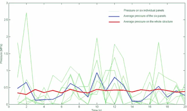
panels and the average pressure over the whole structure are given in Figure 4-2. It can be seen in Figure 4-2 that the effect of the statistical averaging is to reduce the variance of global pressure significantly. This indicates that the use of the measurements based on Medof panels will result in overestimates of the global pressure. Another issue

involved in estimation of ice load, namely, the time under load, has also been investigated. The results are shown in Figure 4-3. The duration of the ice-structure interaction has been varied from 1 minute to 1 hour in this demonstration. It can be seen that the longer the interaction process, the higher is the pressure the structure will experience. This is an important factor in for example a comparison of the Hans Island and Molikpaq data.

Figure 4-2 Pressure trace simulation for 20 seconds. The six green lines are pressure traces of six individual Medof panels. The thick blue line is the average of the six panels and the thick red line is the average pressure over the whole structure.

Figure 4-3 Peak pressure for different loading periods from 1 minute to 1 hour.

4.3 Determination of Global Load Paramters – Molikpaq, Amauligak I-65

4.3.1 Introduction

Ice data from the 1985/1986 season were processed and organized into MATLAB binary files by reading text data files. The Medof panel forces are analyzed on a probabilistic basis to assess their characteristics (probability distribution, mean, standard deviation, and correlation structure in space). The following should be noted:

• The data shows that Medof panel forces correlate on adjacent panels while they do not correlate on detached panels.

• A Markov assumption is therefore used in this study.

• It is assumed that ice loading follows a first-order autoregressive process in space. Based on this assumption, a correlation parameter of 0.5 to 0.9 can be estimated from the correlation coefficients of the adjacent panels.

• Two values of “c” (see below) were examined based on typical values of

correlation coefficient ρ as calculated for adjacent panels:

If ρ = 0.6,c is approximately equal to 0.82.

4.3.2 Methodology

The data included 80 series collected in major ice interaction events. Medof panel forces were analyzed based on a probabilistic basis to assess their probabilistic characteristics such as the probability distribution, mean, standard deviation, and correlation structure in space.

In a process in time, an event of a Markov process depends on the previous one and not those earlier in the process (“knowledge of the present makes the future independent of the past”). The correlation is directional because time moves forward only. A process in space is distinct from a process in time: there is no preference of directionality. The following event correlates to both the preceding one and the following one. This can be expressed by the second-order difference equation:

[

]

(t a X t X t U t

X = − + + + , 4.1

where X(t)is the random series and the a is a constant and U(t) is an uncorrelated

random series. The associated covariance function is

c x x c e B 2 / ) 1 / ( ) (τ =σ τ + −τ . 4.2

where σ_x2 is the variance and τ is the lag distance (noting that space rather than time is

the key variable) which is the distance between two points, for instance adjacent panels (at a spacing of 1.13 m).

The first-order autoregressive model has an exponential correlation function

c e c / 1 ) (τ τ τ ρ − ⎥ ⎦ ⎤ ⎢ ⎣ ⎡ + = 4.3

where c is a constant which can be calculated based on the correlation coefficient and distance between adjacent panels. The value of c is ~1.37m for a correlation coefficient equal to 0.8. To estimate mean and standard deviation of ice pressure, first the line load is calculated using Medof panel forces. For the line load calculation, loaded panels are noted. The loads on the loaded Medof panel forces are summed up and then divided by number of columns of loaded Medof panels and the width of panels (1.13m). Ice

thickness and the line load for known events, the mean and standard deviation of ice pressures are calculated.

Ice pressure generally follows an exponential distribution for local areas. For large areas, a Gaussian distribution follows as a result of the central theorem. Using this assessment, ice pressure is modelled as a random averaging process with a Gaussian distribution, defined by a mean and standard deviation and a first-order autoregressive correlation function in space.

Using the above model, global ice pressure on a large contact area can be

probabilistically defined. Global ice pressure has a mean equal to mean of local ice pressure. Its standard deviation reduces depending on size of the loaded area. The

variance σ_T2 after averaging of a one-dimensional random process with variance σ2 is

2 2 ) ( σ γ σ_T = T 4.4

where T is the averaging distance which is taken as the whole structure width in this case

and the variance function γ(T) is defined (Vanmarke, 1983) as

∫

The square root of the variance function,

[

]

the point standard deviation σ .

For a first-order autoregressive model, the reduction function for one-dimensional space is ⎟ ⎟ ⎠ ⎞ ⎜ ⎜ ⎝ ⎛ − − + = − − ) 1 ( 3 2 2 ) ( / c T c T e T c e T c T γ 4.6

The above methodology applied to the Molikpaq data yielded a local ice pressure is

estimated to have a mean of µ = 0.23 MPa and a coefficient of variation (CV) = 1.06.

The global ice pressure on a area 90 m wide has a mean of 0.23 MPa and standard deviation of 0.044 MPa or 0.042 MPa when “c” is taken as 0.82 or 1.4 respectively The mean and standard deviation of the local ice pressure is first estimated for each event. This is done by first calculating the line load of the event using the Medof panel data (modified Timco and Johnston (2003) method), and requires that loaded Medof

panel forces be summed up for each event and then divided by number of columns of loaded Medof panels and the width of panels (1.13m). Ice thickness is known for certain ice events as reported by Rogers et al., 1998. Using the ice thickness and line load, an event average pressure data series is produced.

4.3.3 Illustrative Example

This section describes in more detail how the above methodology was applied. The event

of March 8th, 1986 (fast file f603081731) is used as an example. This file contains data

for the following load panels; 1002, 1003, 1004, 1006, 1007, 1008, 1009, 1010, 1011, 1012, 1013, 1014, 1018, 1020. (see Figure 2-1 and Figure 4-4).

Figure 4-4 Loaded Medof panels used in analysis fast file f603081731, note that 8 columns (vertical cross sections), and 14 panels are loaded.

4.3.3.1 Convert the data into a useable format.

The nature of the Medof panels leads to inconsistent zero baselines that can be described as “floating”; this means that the data from each panel has to be normalized. This is done by inspecting the data in plotted form and then adjusting it back to zero based on the lowest point either before the loading initiates or after it has stopped (Figure 4-5).

Figure 4-5 Medof data, fast file f603081731; this shows individual load data for 14 loaded panels after zeroing.

4.3.3.2 Produce an event average pressure data series

Once the data has been normalized (zero’d), the event data (one series for each loaded panel) are averaged to produce an event average column curve. The load series is then converted into an event average pressure curve. The area considered is the width of a single panel multiplied by the number of columns loaded (a column is a vertical stack of panels, event from Figure 4-4 it can be seen that event f603081731 has 8 columns) multiplied by the observed thickness of the ice during the event. The average of the

0 500 1000 1500 2000 2500 3000 3500 4000 -100 0 100 200 300 400 500 600 700 800 Time (s) P ane l F orc e (t onn es ) f603081731med 1002 1003 1004 1006 1007 1008 1009 1010 1011 1012 1013 1014 1018 1020

observed minimum thickness and observed maximum thickness was used. This is seen in the first graph of Figure 4-6.

4.3.3.3 Trim the event average pressure curve and calculate the mean and standard distribution.

The average pressure curves were plotted, and any gaps in the data, including excessive tail data were trimmed. This leaves a continuous data series of pressures for each event. The product of this is that a standard deviation and a mean can be calculated to be used in the further analysis (second graph in Figure 4-6). This is done for each event individually (see appendix A for all event graphs).

Figure 4-6 : Average pressure graphs for fast file f603081731

Untrimmed Data

µ

µ

•

•

•

Data trimmed for analysis

4.3.3.4 Calculate the standard deviation for individual columns from groups of contiguous panels and for global pressure for each event—Method 1

By applying the methodology described in section 4.3.2 above it is now possible to calculate a standard deviation for the individual column pressure distribution. In Method

1, a set of adjacent Medof panels are considered. The factor

γ

using the autoregressive methods outlined above.

In the case of event f603081731 the standard deviation of the average column pressure is 0.1137 MPa (Figure 4-6) resulting in

1. If c = 1.4, the individual column standard deviation is 0.165 MPa and, 2. If c = 0.82, the individual column standard deviation is 0.203 MPa.

As can be seen from Tables 4-2 and 4-3, the

γ

column pressure standard deviation are unique to each event. This is because it is related to the actual loaded length, which is also unique to each event.

The global

γ

pressure standard deviation to calculate a global pressure standard deviation. In the case of event f603081731 the global pressure standard deviations are:

1. If c = 1.4, the global standard deviation is 0.041 MPa and, 2. If c = 0.82, the global standard deviation is 0.0385 MPa.

For calculating global pressure standard deviation, the actual loaded length is not needed and T = 90 m (the global length in the case of the Molikpaq) is constant for all events. It

can be seen from Tables 4-2 and 4-3, that this results in the global

γ

constant for all events.

The results for the data series investigated are presented in Tables 4-2 and 4-3 (for,

4.3.3.5 Calculate the standard deviation for an individual column from groups of two adjacent columns and for global pressure for each event—Method 2

In this case, a similar methodology to that in sections 4.3.2 and 4.3.3.4 above was used. The standard deviation of pairs of adjacent columns was related to that of individual columns using autoregressive methods. Then the results for pairs of columns were combined assuming independence between pairs. The standard deviation of pressure distribution for a group (say four) of two adjacent columns can then be used to calculate the standard deviation.

In the case of event f603081731 the standard deviation of the average column pressure is 0.1137 MPa (Figure 4-6) resulting in

1. If c = 1.4, the standard deviation of column pressure for two adjacent columns is 0.233 MPa and,

2. If c = 0.82, the standard deviation of column pressure for two adjacent columns is 0.239 MPa.

As can be seen from Tables 4-4 and 4-5, the

γ

standard deviations is constant between each event. This is because it is related to the distance from center to center of two adjacent panels, which is constant for all pairs of columns in all events.

The calculation of the reduction factor was conducted whereby the square root of the

local

γ

between pairs). Where the number of loaded groups represents the number of panel clusters that had a loaded column within, i.e. in the case where at least 1 of 2 columns in a group is loaded, it is considered to be a loaded group.

The global

γ

standard deviation for two adjacent columns to calculate a global pressure standard deviation. In the case of event f603081731 the global pressure standard deviations are:

1. If c = 1.4, the global standard deviation is 0.057 MPa and, 2. If c = 0.82, the global standard deviation is 0.045 MPa.

For calculating global pressure standard deviation, the actual loaded length is not needed in this case and T = 90 m (the global length in the case of the Molikpaq) is constant for

all events. It can be seen from Tables 4-4 and 4-5, that this results in the global

γ

The results for the data series investigated are presented in Tables 4-4 and 4-5 (for,

ρ(τ) = 0.8, c = 1.4 and ρ(τ)=0.6, c = 0.82 below.

4.3.3.6 Calculate the standard deviation for a group of two adjacent columns using a linear function of random quantities and for global pressure for each event— Method 3

By considering a linear function of random quantities, as described below, it is possible to calculate the standard deviation of pressure distribution for a group of two adjacent columns. If U = aX + bY, where both X and Y have a joint probability distribution, the variance can be formulated as

(

)

X

X

(

) ( )

( )

σ

σ

(

)

In the case of event f603081731, the standard deviation of the average column pressure is 0.1137 MPa (Figure 4-6) resulting in

1. If ρ = 0.8, the standard deviation of column pressure for two adjacent

columns is 0.240 MPa and,

2. If ρ = 0.6, the standard deviation of column pressure for two adjacent

columns is 0.255 MPa.

The calculation of the reduction factor was calculated using the square root of the value

obtained from ½(1+ρ) divided by the number of loaded groups. Where the number of

i.e. in the case where at least 1 of 2 columns in a group is loaded, it is considered a loaded group.

The global

γ

standard deviation for two adjacent columns to calculate a global pressure standard deviation. In the case of event f603081731 the global pressure standard deviations are:

3. If c = 1.4, the global standard deviation is 0.059 MPa and, 4. If c = 0.82, the global standard deviation is 0.048 MPa.

For calculating global pressure standard deviation, the actual loaded length is not needed and T = 90 m (the global length in the case of the Molikpaq) is constant for all events. It

can be seen from Tables 4-4 and 4-5, that this results in the global

γ

constant for all events.

The results for the data series investigated are presented in Tables 4-6 and 4-7 (for,

Table 4-1: The mean and standard deviation of events calculated with modified line load method. “Local” standard deviation refers to that of the Mean Average Pressure on the Columns.

Filename Date Duration

(min) Usable Duration (min) Min. Ice Thickness (m) Max Ice Thickness (m) Average Ice Thickness (m) Mean Average Pressure (MPa) on the Columns Local S.D f601071801med.txt 7 Jan 1986 65.2490 46.7000 1 1.5 1.25 0.109 0.045 f602062201med.txt 6 Feb 1986 65.5803 65.0830 0.8 1.2 1 0.2007 0.139 f602070301med.txt 7 Feb 1986 65.2852 65.2852 0.9 1.2 1.05 0.2164 0.146 f602072301med.txt 7 Feb 1986 65.3162 65.3162 0.9 0.9 0.9 0.3579 0.124 f602080101med.txt 8 Feb 1986 65.5928 35.3000 0.9 1.2 1.05 0.2921 0.198 f602080201med.txt 8 Feb 1986 65.0317 65.0317 0.9 1.2 1.05 0.1915 0.119 f602171600med.txt 17 Feb 1986 29.4915 29.4915 0.7 0.8 0.75 0.3492 0.099 f602280821med.txt 28 Feb 1986 65.3110 43.3000 0.8 0.9 0.85 0.3776 0.199 f605220801med.txt 22 May 1986 73.6600 73.6600 2 3 2.5 0.2454 0.091 f605221301med.txt 22 May 1986 74.5400 75.5400 2 3 2.5 0.2285 0.148 f606021301med.txt 2 Jun 1986 74.7500 74.7500 1.8 2.5 2.15 0.4492 0.174 f606022001med.txt 2 Jun 1986 68.5500 45.5000 1.8 2.5 2.15 0.2712 0.109 f511101401repairedmed.txt 10 Nov 1985 65.0253 50.0000 0.5 1.5 1 0.1537 0.133 f511271201med.txt 27 Nov 1985 65.1412 51.7000 1.2 1.2 1.2 0.2377 0.131 f512160801med.txt 16 Dec 1985 65.0668 28.3000 1.2 1.2 1.2 0.2878 0.169 f605120301med.txt 12 May 1986 72.0472 46.1500 1.5 3.5 2.5 0.3287 0.140 f603071520med.txt 7 Mar 1986 71.0500 71.0500 3.5 10 6.75 0.1151 0.050 f603071603med.txt 7 Mar 1986 65.7892 42.0000 3.5 10 6.75 0.0905 0.044 f603081603med.txt 8 Mar 1986 71.2090 29.1300 3.7 4 3.85 0.0939 0.095 f603081731med.txt 8 Mar 1986 65.5500 48.7000 3.7 4 3.85 0.3296 0.114 f603082101med.txt 8 Mar 1986 71.3370 71.3370 3.7 4 3.85 0.032 0.017 f603082201med.txt 8 Mar 1986 36.1222 20.3700 3.7 4 3.85 0.08983 0.007 f603251302med.txt 25 Mar 1986 130.2463 130.2400 2.75 2.75 2.75 0.1804 0.091 f604121101med.txt 12 Apr 1986 74.5185 42.0000 3.6 3.6 3.6 0.2974 0.246 f604121201med.txt 12 Apr 1986 74.0685 15.1700 3.6 3.6 3.6 0.213 0.172 f604121400med.txt 12 Apr 1986 16.5913 16.5900 3.6 3.6 3.6 0.2236 0.079 Average 0.2293 0.118

Table 4-2Table showing the results and methodology for calculating a new standard

deviation for the individual columnand global standard deviation based on ρ = 0.6 and

c = 0.82. Method 1. Filename Date # of Columns Actual loaded length (m) Local γ(Τ) c = 0.82 T = actual loaded length Individual Column S.D. (MPa) Global γ (Τ) c = 0.82 T = 90 m Global S.D. (MPa) f601071801med.txt 7 Jan 1986 14 15.82 0.191212 0.102909 0.03594637 0.0195 f602062201med.txt 6 Feb 1986 8 9.04 0.313468 0.248267 0.03594637 0.0471 f602070301med.txt 7 Feb 1986 8 9.04 0.313468 0.260055 0.03594637 0.0493 f602072301med.txt 7 Feb 1986 14 15.82 0.191212 0.284258 0.03594637 0.0539 f602080101med.txt 8 Feb 1986 8 9.04 0.313468 0.354182 0.03594637 0.0672 f602080201med.txt 8 Feb 1986 8 9.04 0.313468 0.212366 0.03594637 0.0403 f602171600med.txt 17 Feb 1986 14 15.82 0.191212 0.225486 0.03594637 0.0428 f602280821med.txt 28 Feb 1986 14 15.82 0.191212 0.455545 0.03594637 0.0864 f605220801med.txt 22 May 1986 14 15.82 0.191212 0.208105 0.03594637 0.0395 f605221301med.txt 22 May 1986 14 15.82 0.191212 0.339372 0.03594637 0.0643 f606021301med.txt 2 Jun 1986 6 6.78 0.396096 0.275994 0.03594637 0.0523 f606022001med.txt 2 Jun 1986 8 9.04 0.313468 0.194505 0.03594637 0.0369 f511101401repairedmed.txt 10 Nov 1985 6 6.78 0.396096 0.211802 0.03594637 0.0402 f511271201med.txt 27 Nov 1985 8 9.04 0.313468 0.233621 0.03594637 0.0443 f512160801med.txt 16 Dec 1985 7 7.91 0.350202 0.285749 0.03594637 0.0542 f605120301med.txt 12 May 1986 14 15.82 0.191212 0.320848 0.03594637 0.0608 f603071520med.txt 7 Mar 1986 8 9.04 0.313468 0.089662 0.03594637 0.0170 f603071603med.txt 7 Mar 1986 8 9.04 0.313468 0.078052 0.03594637 0.0148 f603081603med.txt 8 Mar 1986 8 9.04 0.313468 0.170393 0.03594637 0.0323 f603081731med.txt 8 Mar 1986 8 9.04 0.313468 0.203078 0.03594637 0.0385 f603082101med.txt 8 Mar 1986 5 5.65 0.454574 0.025659 0.03594637 0.0049 f603082201med.txt 8 Mar 1986 7 7.91 0.350202 0.012194 0.03594637 0.0023 f603251302med.txt 25 Mar 1986 13 14.69 0.204586 0.20141 0.03594637 0.0382 f604121101med.txt 12 Apr 1986 4 4.52 0.530455 0.337762 0.03594637 0.0640 f604121201med.txt 12 Apr 1986 6 6.78 0.396096 0.273452 0.03594637 0.0518 f604121400med.txt 12 Apr 1986 6 6.78 0.396096 0.126223 0.03594637 0.0239 Average 0.0418

Table 4-3 Table showing the results methodology for calculating a new standard

deviation for the individual columnand global standard deviation based on ρ = 0.8 and

c = 1.4. Method 1. Filename Date # of Columns Actual loaded length (m) Local γ(Τ) c = 1.4 T = actual loaded length Individual Column S.D. (MPa) Global γ (Τ) c = 1.4 T = 90 m Global S.D. (MPa) f601071801med.txt 7 Jan 1986 14 15.82 0.306996271 0.081216817 0.06077037 0.0200 f602062201med.txt 6 Feb 1986 8 9.04 0.476277705 0.20141169 0.06077037 0.0497 f602070301med.txt 7 Feb 1986 8 9.04 0.476277705 0.210975123 0.06077037 0.0520 f602072301med.txt 7 Feb 1986 14 15.82 0.306996271 0.224338896 0.06077037 0.0553 f602080101med.txt 8 Feb 1986 8 9.04 0.476277705 0.287337685 0.06077037 0.0708 f602080201med.txt 8 Feb 1986 8 9.04 0.476277705 0.17228669 0.06077037 0.0425 f602171600med.txt 17 Feb 1986 14 15.82 0.306996271 0.17795507 0.06077037 0.0439 f602280821med.txt 28 Feb 1986 14 15.82 0.306996271 0.359519775 0.06077037 0.0886 f605220801med.txt 22 May 1986 14 15.82 0.306996271 0.164238452 0.06077037 0.0405 f605221301med.txt 22 May 1986 14 15.82 0.306996271 0.267835013 0.06077037 0.0660 f606021301med.txt 2 Jun 1986 6 6.78 0.575403993 0.228988347 0.06077037 0.0564 f606022001med.txt 2 Jun 1986 8 9.04 0.476277705 0.157796641 0.06077037 0.0389 f511101401repairedmed.txt 10 Nov 1985 6 6.78 0.575403993 0.175729112 0.06077037 0.0433 f511271201med.txt 27 Nov 1985 8 9.04 0.476277705 0.18952985 0.06077037 0.0467 f512160801med.txt 16 Dec 1985 7 7.91 0.521915672 0.234068751 0.06077037 0.0577 f605120301med.txt 12 May 1986 14 15.82 0.306996271 0.253215986 0.06077037 0.0624 f603071520med.txt 7 Mar 1986 8 9.04 0.476277705 0.072740049 0.06077037 0.0179 f603071603med.txt 7 Mar 1986 8 9.04 0.476277705 0.063321517 0.06077037 0.0156 f603081603med.txt 8 Mar 1986 8 9.04 0.476277705 0.138235074 0.06077037 0.0341 f603081731med.txt 8 Mar 1986 8 9.04 0.476277705 0.164751865 0.06077037 0.0406 f603082101med.txt 8 Mar 1986 5 5.65 0.638027184 0.021658407 0.06077037 0.0053 f603082201med.txt 8 Mar 1986 7 7.91 0.521915672 0.00998841 0.06077037 0.0025 f603251302med.txt 25 Mar 1986 13 14.69 0.326722619 0.159378148 0.06077037 0.0393 f604121101med.txt 12 Apr 1986 4 4.52 0.710667272 0.291811195 0.06077037 0.0719 f604121201med.txt 12 Apr 1986 6 6.78 0.575403993 0.226879071 0.06077037 0.0559 f604121400med.txt 12 Apr 1986 6 6.78 0.575403993 0.104725586 0.06077037 0.0258 Average 0.0440