Boron neutron capture therapy treatment planning improvements

Boron Neutron Capture Therapy

Treatment Planning Improvements

by

John Timothy Goorley B.S. Nuclear Engineering B.S. Radiological Health Engineering

Texas A&M University (1996)

Submitted to the Department of Nuclear Engineering in partial fulfillment of the requirements for the degree of

Masters of Science in Nuclear Engineering at the

Massachusetts Institute of Technology June 1998

Copyright @ Massachusetts Institute of Technology, 1998. All Rights Reserved.

Author ...

1'

Boron Neutron Capture Therapy

Treatment Planning Improvements

by

John Timothy Goorley

Submitted to the Department of Nuclear Engineering on May 19, 1998, in Partial Fulfillment of the Requirements for the

Degree of Masters of Science in Nuclear Engineering

Abstract

The Boron Neutron Capture Therapy (BNCT) treatment planning process of the Harvard/MIT team used for their clinical Phase I trials is very time consuming. If BNCT proves to be a successful treatment, this process must be made more efficient. Since the Monte Carlo treatment planning calculations were the most time consuming aspect of the treatment planning process, requiring more than thirty six hours for scoping calculations of three to five beams and final calculations for two beams, it was targeted for improvement. Three approaches were used to reduce the calculation times. A statistical uncertainty analysis was performed on doses rates and showed that a fewer number of particles could not be used and still meet uncertainty requirements in the region of interest. Unused features were removed and assumptions specific to the Harvard/MIT BNCT treatment planning calculations were hard wired into MCNP by Los Alamos personnel, resulting in a thirty percent decrease in runtimes. MCNP was also installed in parallel on the treatment planning computers, allowing a factor of improvement by roughly the number of computers linked together in parallel. After theses enhancements were made, the final executable, MCNPBNCT, was tested by comparing its calculated dose rates against the previously used executable, MCNPNEHD. Since the dose rates in close agreement, MCNPBNCT was adopted. The final runtime improvement to a single beam scoping run by linking the two 200MHz Pentium Pro computers was to reduce the wall clock runtime from 2 hours thirty minutes to fifty nine minutes. It is anticipated that the addition of ten 900 MHz CPUs will further reduce this calculation to three minutes, giving the medical physicist or radiation oncologist the freedom to use an iterative approach to try different radiation beam orientations to optimize treatment.

Additional aspects of the treatment planning process were improved. The previously unrecognized phenomenon of peak dose movement during irradiation and its potential for overdosing the subject was identified. A method of predicting its occurrence was developed to prevent this from occurring. The calculated dose rate was also used to create dose volume histograms and volume averaged doses. These data suggest an alternative method for categorizing the subjects, rather than by peak tissue dose.

Thesis Supervisor: Guido R. Solares

Title: Assistant Professor of Radiology at Harvard Medical School Thesis Reader: Jacquelyn C. Yanch

Title: Associate Professor of Nuclear Engineering and Whitaker College of Health Sciences and Technology Thesis Reader: Robert Zamenhof

Acknowledgments

I would like to thank my thesis advisor, Dr. Guido Solares for his effort and help. I wish

him the best in his new pursuits.

I appreciate the helpful thesis review and suggestions given by Dr. Yanch, Dr. Zamenhof, and W.S. Kiger. Thanks for your time and attention.

I greatly appreciate Dr. G. McKinney's personal assistance and supervision of my work at Los Alamos and MIT.

I wish to thank the BNCT group members W.S. Kiger, C. Chuang, K. Riley, M.

Ledesma, Dr. R. Zamenhof, Dr. M. Palmer, Dr. P. Busse, Dr. O. Harling, Dr. L.Tang, J. Kaplan, and Dr. I. Kaplan. This group of people has helped make my experience with the

BNCT project a personally rewarding academic learning experience.

I would like to thank the Los Alamos National Laboratory personnel that have been

extremely helpful. Dr. G. McKinney, Dr. K. Adams and Dr. G. Estes have been supportive during my various stays at Los Alamos and through my other contact with them. I also wish to say thanks to all of the other XTM and XCI personnel that have increased my understanding of MCNP: Dr. J. Hendricks, Dr. J. Briesmeister, and the other instructors I have learned from.

I would like to thank the MIT Reactor personnel for their help with the project. Dr. J. Bernard, T. Newton, and F. Mc Williams have been particularly gracious.

This research was supported by the U. S. Department of Energy contract

W-7405-ENG-36 with the University of California (Los Alamos National

Laboratory) and grant #DE-FG02-97ER62193 with the Beth Israel Deaconess Medical Center.

Table of Contents Page Abstract 2 Acknowledgments 3 Table of contents 4 List of figures 6 List of tables 7 1. Introduction 8 2. Harvard/MIT BNCT Treatment 9 2.1 Treatment process 9 2.1.1 Beam Characterization 11 2.1.2 Treatment Planning 13 2.1.3 Irradiation Procedure 15

2.1.4 Laptop Retrospective Dosimetry 16 2.1.5 MCNP Retrospective Dosimetry 17

2.2 Treatment planning process 18

2.2.1 Preparation 19 2.2.2 MacNCTPlan Part I 23 2.2.3 MPREP 27 2.2.4 MCNP Calculations 28 2.2.5 MacNCTPlan Part II 28 2.2.6 MCNP Input Deck 30

2.3 Monte Carlo N Particle Radiation Transport Code 31

2.3.1 Lattice Model 31

2.3.2 Non Lattice Model 34

2.3.3 Materials 35

2.3.4 Neutron and Photon Source 38

2.3.5 Flux Tallies 42

2.3.6 Flux to dose multipliers 42

3. Treatment Planning MCNP Run Time Reductions 48

3.1 Uncertainty analysis 49

3.1.1 Voxel Dose Uncertainty Analysis 49 3.1.2 Isodose Rate Contour Analysis 52 3.2 MCNP source code enhancements 55

3.2.1 Tracking and Tallying Patch 55

3.2.2 Lahey FORTRAN 90 56 3.2.3 GNU 77 57 3.3 Parallel calculations 57 3.3.1 Linux Installation 58 3.3.2 PVM Installation 58 3.3.3 MCNP parallel version 58

3.3.4 Speedup Results 59 3.3.3 Running MCNP in Parallel 61 3.3.4 Job Identification and Importance 62 3.4 Validation of calculation enhancements 64

3.4.1 MCNP4B test suite 64

3.4.2 MCNPNEHD MCNPBNCT Dose Rate Comparison 67 4. Investigation of peak dose location movement during subject irradiation

and dosimetry effects 72

4.1 Identification 73

4.2 Explanation 73

4.2 Prediction 79

4.3 Chapter Conclusions 82

5. Retrospective volume dosimetry calculations and effects 84

5.1 Dose volume histogram calculation 84 5.2 Dose volume histogram results 86

5.3 Volume Averaged Dose 90

5.4 Relation to Peak Dose 91

5.5 Proposed Grouping 92

5.6 Peak Tissue and Peak Brain Doses 94

6. Conclusions 96

Appendices

List of figures

Figure 2.1a. Thermal Neutron Dose Profile 12 Figure 2.lb. Fast Neutron Dose Profile 12 Figure 2.1c. 'oB Depth Dose Profile 13 Figure 2.1d. Photon Depth Dose Profile 13 Figure 2.2 Mapping 16 bit images into 8 bit images 20

Figure 2.3 I+ Imported Images 20

Figure 2.4 Metal Filling Artifacts and Replacement 22 Figure 2.5 I-, I+, Gd+ Images of the same plane with fiducial markers 23 Figure 2.6 Screen Shot of MacNCTPlan Tumor Outlining 24 Figure 2.7 Screen Capture of MacNCTPlan Thresholding 25 Figure 2.8 MacNCTPlan Screen Capture of Beam Positioning 26 Figure 2.9 MacNCTPlan CT Voxelization 27 Figure 2.10 Sabrina 3-D representation of the head model 28 Figure 2.11 Illustration of Multiple Universe Levels 32 Figure 2.12 MCNP Lattice cells and surfaces 33 Figure 2.13 MCNP non-lattice cells and surfaces 35 Figure 2.14 Materials Cards in MCNP BNCT treatment planning input deck 36 Figure 2.15 Particle Creation Modifiers for a Cylindrical Source 39 Figure 2.16 Correlated distributions in a hypothetical BNCT disk gamma source 40 Figure 2.17 Correlated distributions in a hypothetical neutron disk source 41 Figure 2.18 Dose Cards in MCNP BNCT treatment planning input deck 43 Figure 3.1 Total dose rate uncertainty for various number of histories 51 Figure 3.2a Subject 97-3 Two Hundred Fifty Thousand Particles 53 Figure 3.2b Subject 97-3 Five Hundred Thousand Particles 53 Figure 3.2c Subject 97-3 One Million Particles 53 Figure 3.2d Subject 97-3 Three Million Particles 53 Figure 3.2e Subject 97-3 Ten Million Particles 54 Figure 3.3 Total wall clock runtimes for a single beam evaluation 60 Figure 3.4a-d Representation of Jobs and Optimization 63 Figure. 3.5 MCNP Dose Rate Comparison 68 Figure. 3.6 Comparison of Error for each non-air voxel 69 Figure 4.1 Subject 96-4 Chronological Dose Reconstruction 75 Figure 4.2 Enlargement of Fig 4.1. Near EOI 76 Figure 4.3 Subject 97-3 Chronological Dose Reconstruction 77 Figure 4.4 Enlargement of Figure 4.3 near EOI 78 Figure 5.1 Subject Brain Tissue Dose Volume Histograms 86

Figure 5.2 Higher Dose Region DVH 87

Figure 5.3 Tumor Dose Volume Histogram 89

Figure 5.4 Tumor and Tissue DVHs 90

Figure 5.5 Dual Irradiation with close entry locations 91 Figure 5.6 Dual Beam Irradiation with distant entry locations 92

List of tables

Table 2.1 Scaling Factors for the June 1997 Characterization 13 Table 3.1 MCNP Material Composition Fractions 37 Table 3.2 MCNP Wall Clock Run Times 56 Table 3.3 Wall clock run times, in minutes, for a single beam evaluation 59 Table 3.4 MCNP Speedup Summary -Total Wall Clock Runtimes 61 Table 3.5 Non-Zero Difm Files from MCNP4B on Linux 65 Table 3.6 Non-Zero Difm Files from MCNP4B -o2 on Linux 67 Table 4.1 Flip times for Subject 96-4 80 Table 4.2. Subject Dose Rate Contributions (DCR) 81 Table 4.3 Subject's Dose Estimation 82 Table 5.1 DVH Spread Sheet for Subject 97-2 85 Table 5.2 Example Spread Sheet for Tumor DVH Calculation 88

Table 5.3 Subject Max Dose Ratios 92

Table 5.4 Proposed Subject Dose Cohorts 93 Table 5.5 Peak Doses to Various Tissues 94

1. Introduction

Treatment planning is an integral yet time consuming part of the Harvard/MIT Boron Neutron Capture Therapy (BNCT) Phase I clinical trials. If the clinical trials show efficacy of this experimental treatment, and BNCT becomes a mainstream treatment, the treatment planning must be streamlined. In chapter one of this thesis, the treatment planning procedure is described, providing a written record for the reader. Chapters two, three, and four contain the accomplishments of this thesis work. Chapter two details the methods used to greatly reduce the computational time needed in treatment planning: a voxel dose rate error analysis, modifications to the Monte Carlo computer code, and implementation of parallel computing. Also described are the quality assurance tests used to verify the code.

During this thesis research, a previously unrecognized phenomenon of peak dose movement was identified as having occurred in several of the subject irradiations. Further investigation shows a relation between slight subject overdoses and this phenomenon. This effect was also investigated with relation to the beam geometry of the treatment, either perpendicular or nearly parallel opposed. A method of predicting when this global maximum movement occurs was developed. This phenomenon is described in chapter four.

The retrospective dosimetry calculations for this thesis include dose volume histograms and volume averaged doses. These new volume averaged doses could be used as the basis for reorganizing the subject cohorts, rather than on the peak dose, as required by the existing FDA-approved clinical protocol. Additional calculations produced the difference between peak dose to tissue and peak brain dose. These results are described in chapter five.

2. Harvard/MIT BNCT Treatment

Boron Neutron Capture Therapy (BNCT) was first suggested by Gordon Locher in 1936'. Through the application of a boron containing pharmaceutical that is selectively absorbed by a tumor, the tumor receives more dose than the surrounding tissue during subsequent neutron irradiation2'3'4. The increase in dose is caused by the short range of the alpha and 7Li reaction products from neutron absorption by a 'oB nucleus. This process is currently being investigated by several teams around the globe in the treatment of a variety of cancers5'6. The Beth Israel Deaconess Medical Center / MIT group is currently engaged in Phase I clinical trials using the M.I.T. Nuclear Reactor Laboratory's epithermal neutron beam to study the toxicity of neutron irradiation on neural tissue7'8. After the phase I study has been completed, it is hoped that a phase II study will show the efficacy of BNCT for controlling Glioblastoma multiforme and metastatic melanoma.

2.1 Treatment Process

The BNCT treatment process includes a variety of steps in addition to the physical irradiation of a subject. Beam characterization, treatment planning, online dosimetry, and retrospective dosimetry are all parts of the BIDMC/MIT procedure. Each one of these topics is described in detail in this chapter. Beam characterization is necessary to ensure the proper dose is delivered during irradiation. Treatment planning optimizes the radiation dose to tissue and tumor. Retrospective dosimetry verifies the proper dose was delivered during the irradiation procedure and is used to correlate effects, such as tumor regression or reoccurrence, or healthy tissue neurological effects, with delivered dose.

The MIT Nuclear Reactor Laboratory's current epithermal neutron beam, m67, is characterized every six months9. The fast and thermal neutron and gamma dose rates are measured at various depths of an ellipsoid head phantom. The 'lB dose rates are calculated from the thermal neutron flux. The m67 beam is also equipped with two thermal and epithermal neutron detectors, called the beam monitors. The dose rates are proportional to the beam monitor count rates, which are monitored during subject

irradiation. After a calibration is completed, the first stage of the treatment process does not occur until a human subject has been accepted into the protocol.

Treatment planning is the most time consuming aspect of the entire process, taking a minimum of five days to complete even though the actual irradiation takes only a few hours. The treatment planning software, MacNCTPlan, designed and developed at Harvard/MIT, uses CT and MRI data to allow the medical physicist to specify the location of tumor and normal neural tissue, construct a subject specific individual model for radiation transport, and visualize dose rate data from the transport calculations' 1 1 '2. During the several days prior to the irradiation, the medical physicist compares the dosimetric result of using different irradiation beam orientations and selects the final beam geometry. Comparisons are based on dose to sensitive locations as well as maximum, minimum, and dose-volume distributions to tumor and normal tissue. These evaluations are based on calculated dose rates from Monte-Carlo simulation of the irradiation. Once the final beam is selected, a more lengthy calculation is performed to reduce the associated statistical error, since the resultant dose rates will be used to determine the length of irradiation.

The Monte Carlo program MCNP1'3 is used to calculate the dose rates throughout the head phantom and the subject for various beam orientations. MCNP is used for a variety of reasons, including its ability to model the subject, represent the epithermal neutron beam's energy and radial distributions and the complex thermalization process of epithermal neutrons 4.

Once the final beam or beams are determined, there is a distinct change in the dosimetry approach, instigated by the written directive of this Phase I protocol. No longer are doses to various locations considered; only the maximum dose to tissue is important, since the subjects are divided into cohorts on this basis. Since the dose contribution from the 'OB reaction is roughly one quarter of the total dose to normal tissue, an accurate dosimetry protocol must account for the subject 'oB biodistribution during the time of irradiation. Accordingly, the blood 'oB concentration is measured with inductively coupled plasma atomic emission spectrometry (ICP-AES) or prompt gamma

neutron activation analysis (PGNAA), and the total integral dose to the maximum dose location is determined during irradiation. This calculation relates the beam monitor readings to the dose rates in phantom and the Monte Carlo calculations of phantom and subject dose rates.

After the irradiation is concluded and the final blood boron concentration curve is determined through the least squares fit of the measured data with a double or triple exponential, retrospective dosimetry focuses on the dose to a variety of locations and volume dose, in addition to the maximum dose location. The average dose to neural tissue, the maximum, minimum and average tumor doses are also of interest.

2.1.1 Beam Characterization

The neutron and gamma dose rates of the MIT Nuclear Reactor Laboratory's epithermal beam are measured every six months with an ellipsoid head phantom15'1617

The 'OB component is calculated from the thermal neutron fluxes. The phantom is an acrylic shell filled with water. It has several holes in the bottom, which allow the insertion of a radiation detector. Mixed field dosimetry methods are used to determine the magnitude of each dose component. A dual ion chamber is used to measure the fast and gamma dose rates. The cadmium difference method is used to determine the thermal neutron fluxes. The appropriate kerma factors are applied to determine the dose rates from thermal neutrons and the boron capture reaction. All measurements are taken on the central axis of the phantom at one centimeter intervals. The phantom is aligned with the beam's axis and its apex is located one cm below the ceiling of the medical room. The beam counters measure the neutron flux associated with each set of axial dose rate measurements. The neutron flux varies proportionately with reactor power, which is typically 4.8 MW during the phantom measurements and subject irradiation. The immediate result of this measurement is the correlation of beam count rates with phantom dose rates.

The axial dose rates in phantom are independently calculated by MCNP. Although the dose rates to every 1 cm3 voxel within the 21 cm by 21 cm by 25 cm model of the head phantom can be calculated, only the dose rates along the central axis are compared to the experimental data. In a process similar to the modeling of the subject, which is described later in this chapter, the phantom is modeled in MCNP as a water ellipsoid with the air holes in the bottom where the detectors are inserted. Neutron and photon dose rates are calculated for each cell. The boron dose is determined from the thermal neutron flux in each cell.

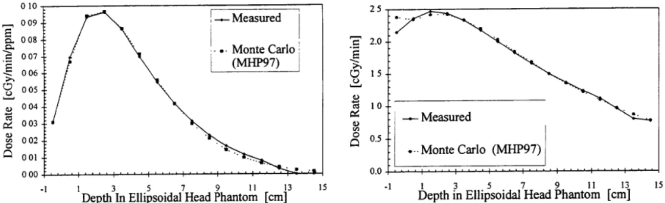
Measured and MCNP calculated dose rates are then plotted as dose rate vs. depth, as shown in Fig 2.1a-e. The fast neutron, thermal neutron and boron dose rates are directly compared. MCNP calculates the dose rates from the structural gammas and induced, or capture gammas, individually, which are compared to the measured gamma dose rate, or the sum of the two.

Figs. 2.1 a-d show the adjusted MCNP phantom dose rates and experimental data for the June 1997 characterization'8.

0.18 2.5

0.16 .-.- Measured

' 0.14 20

S0.12 --.... Monte Carlo (MHP97) _{Carlo (IMHP97)}

S0.08 0 o10o S00 6 0.04 _o.s0 0.02 0.00 _{.... .0.0} -1 1 3 5 7 9 11 13 15 -1 1 3 5 7 9 11 13 15

Depth in Ellipsoidal Head Phantom [cm] DepthIn Ellipsoidal Head Pamtam [an]

010 25 009 -- Measured S008 - 2.0 -S08 *. Monte Carlo S(MHP97) 006 -15 0 05 _ 004 10 004 € -- Measured I 003 -002 0.5 M 0 . Monte Carlo (MHP97) 0000 -1 1 3 5 7 9 11 13 15 -1 1 3 5 7 9 11 13 15

Depth In Ellipsoidal Head Phantom [cm] Depth in Ellipsoidal Head Phantom [cm]

Figure 2.1c. 'OB Depth Dose Profile Figure 2.1d. Photon Depth Dose Profile

Using the dose rate vs. depth data, the least squares difference scaling factor is then found. For the gamma component, a scaling factor for each MCNP dose rate is used. These scaling factors physically account for the difference between experimental dose rates and the calculated MCNP dose rates. With this correction factor, the doses from MCNP can then be considered as the physical dose rates occurring in the subject. Typical scaling factors, shown in Table 2.1, are near unity, indicating that there is a strong agreement between dose rate calculations and measurements.

Table 2.1 Scaling Factors for the June 1997 Characterization Thermal N Fast N '0B Induced y Structural y 0.824 1.088 0.805 0.901 1.810

2.1.2 Treatment Planning

Individualized subject treatment planning begins when a subject enters the protocol. The major steps include MCNP simulation of the irradiation, relation of subject and phantom MCNP dose rate results and calculation of anticipated irradiation time.

The introduction of individualized subject data begins with CT scans and MRIs. These images allow the physician to localize potential tumors, as well as construct a model using subject specific data. As with the phantom data, the images are imported and processed as follows. Within MacNCTPlan, the images are thresholded to

differentiate air, soft tissue and bone, which are included in the model. Several potential beam orientations are designated. MacNCTPlan also voxelizes the subject data into 1 cm3 cells. These data are converted into a MCNP input deck, and MCNP is run to determine the dose rates in each voxel for each beam orientation. Each potential beam is run so that its statistical error is on the order of five percent in the region of interest. One or two final beams are chosen and they are run until the statistical error is around one percent in the region of interest.

The dose rate scaling factors, created by the phantom calibration, are also applied to the subject Monte Carlo data to obtain the representative physical dose rates throughout the subject. The maximum physical dose rates in the phantom and subject are then determined for anticipated boron concentrations, typically 15 and 12 ppm for the first and second beams. The ratio of the maximum of the two dose rates is called the Monte-Carlo Dose Rate Ratio (MCDRR). When the peak dose rate measured in phantom during the axial irradiation is divided by the MCDRR, the result is the physically occurring peak dose rate in the subject from a specific, non axial, radiation beam orientation. Although the MCDRR relates physical dose rates, it is based on the calculated dose rates and the scaling factors, and hence will vary with the curve fit used. Since the MCDRR is a ratio of the dose rates, small fluctuations in scaling factors will have no significant impact on the MCDRR value.

After the final dose rates have been determined, the length of irradiation is estimated. For one beam irradiations, the prescription dose is divided by the maximum dose rate occurring in the subject, or the MCDRR times the maximum phantom dose rate. For a dual beam irradiation, the process is more complex. Using MacNCTPlan, the dose rates from both beams are added, assuming some neutron fluence weighting factor between the first and second beam, as described in section 2.2.5. Once the dose rate distributions of both the beams are added, the maximum dose rate location is calculated. The ratio between a beam's maximum dose rate to the combined global maximum dose rate is calculated. Using this ratio, which accounts for the beam weighting, and the prescription combined global maximum dose, the target dose from each beam is calculated for that beam's peak dose. During the irradiation the beam's peak dose is

determined by the count rates and boron biodistribution as described in the following section.

2.1.3 Irradiation Procedure

The current protocol used by the BNCT group defines the intended target dose, the prescription dose, as the maximum dose occurring within any non-tumor tissue. The maximum dose location will vary with number and orientation of beams, and can occur in scalp, skull or brain. This prescription dose is incrementally increased by ten percent with each new cohort. The previous dose steps have been 880, 990, 1065 RBE cGy.

At various times throughout the infusion and irradiation, 1 ml blood samples are taken to determine the boron concentration. These samples are analyzed with either inductively coupled plasma atomic emission spectrometry or prompt gamma neutron activation analysis'920_{. The resulting biodistribution curve is fit with a double or triple}

exponential.

To ensure the best calculation of subject dose, the cumulative dose is recalculated as the subject's biodistribution curve is measured. There are two methods currently used by the group. The method developed by Dr. Guido Solares allows almost instantaneous dose calculations and evaluations21'22. His computer is taking continuous readings from the beam counters. The second method developed by the group is slightly more discrete. The "laptop" calculations recalculate the cumulative dose to the subject every fifteen minutes, and more frequently near the end of irradiation. These calculations account for the subject's boron biodistribution curve and the effective power of the reactor.

The beam monitors measure the neutron rates and are a direct reflection of reactor power. Reactor power will vary throughout the irradiation, during startup, shutdown and subject repositioning. This variation affects dose rates and the delivered dose during the irradiation. By dividing the beam monitor measurements during subject irradiation by measurements during the phantom irradiation, the effective reactor power is found over a given time interval. When this ratio is divided by the MCDRR, multiplied by the measured phantom dose rates and a particular time interval, the peak dose delivered by

the non-boron components to the subject is calculated. The associated boron dose is multiplied by the average boron concentration during the time interval.

The effective reactor power is used to calculate the effective full power irradiation times and the effective boron concentration for each beam after the irradiation is concluded. These two post irradiation quantities will be used to calculate the retrospective doses from the Monte Carlo dose rates.

2.1.4 Laptop Retrospective Dosimetry

The effective irradiation time for each beam is a measure of full power irradiation time, and is multiplied by the calculated dose rates, scaling factors, and boron concentration to find the delivered dose to any location within the subject model. Equation 2.1 shows that for a dual beam irradiation, the delivered dose to the ith voxel is the sum over the two applied beams, B 1 and B2, of the dose rates multiplied by their respective effective irradiation times.

Dose(i) = DR(i),, B TBI + DR(i)B2 TB2 Equation 2.1

The dose rate, DR(i), in equation one includes the boron dose rate component, which should be multiplied by the beam's effective boron concentration. The effective boron concentration for the first beam, BBEf , is the power weighted time averaged 'oB concentration during a given beam. It is calculated using equation 2.2, where a and b are the beginning and end of the irradiation beam, B(t) is the boron concentration as defined by the final boron biodistribution curve, which includes 'oB concentration measurements several hours after the irradiation has concluded. PEff(t) is the effective power. The other beams are calculated in the same way.

b

B(t ₎ PEf (t) - dt

BER (ppm) = b Equation 2.2

The biodistribution curve, along with the two physical parameters of actual irradiation times and reactor power, are fixed and will not change with dose recalculations, nor will the effective boron concentrations and irradiation times. The post -irradiation values are used by MacNCTPlan in calculating a new MCDRR, which is then used to recalculate the peak dose delivered to the subject in the laptop dosimetry spreadsheet. Since the dose is based on measured values, the retrospective laptop dose is the best estimate of the peak dose delivered.

2.1.5 MCNP Retrospective Dosimetry

Although the phantom measurement based dosimetry provides an accurate peak dose in the phantom, it fails to determine the subject's final dose distribution, which has important clinical significance. While the calculated dose rates are the only current method of determining off axis dose rates, they do rely on the least squares fit of the scaling factors. In cases where the measured and calculated values differ, it is possible to use the calculated dose distributions and infer that the supposed peak dose was significantly higher than was actually delivered. Figure 2.lb shows the calculated fast neutron dose rate at 1 cm is fifteen percent higher than the measured dose rate. However, since the least squares fit is applied over the entire curve, the volumetric dosimetry is a reasonable approximation.

In the retrospective analysis, the doses to tumor and tissue are determined in addition to the maximum dose. Within MacNCTPlan, the neural tissue can be identified and marked in the same manner as the tumor. The volume of neural tissue for each voxel can be determined, as can the total volume of neural tissue in the head. The volumes calculated have been slightly higher than the anticipated values based on ICRP, but tend to agree well with a newly constructed phantom model adopted by the MIRD comittee24 25. Once the volumes of tumor and tissue have been calculated, their corresponding dose distributions can be used for volumetric dosimetry.

The retrospective doses to various locations are determined differently. The peak or prescription dose is best determined with the laptop dosimetry, while average doses

can only be determined with MCNP. Calculation of the volume averaged doses requires knowledge of the three dimensional dose distributions, which is only gained from the MCNP calculations. Currently the depth vs. dose rate distribution along the beam's axis only is obtained from phantom measurements.

Using the dose to each voxel and the fraction of each voxel that is either tumor or tissue, it is possible to calculate the volume of tissue or tumor that receives a certain amount of dose or higher. This plot is referred to as a dose volume histogram, or DVH.

DVHs are used by radiologists to visually determine the advantage dose, or the additional dose the tumor receives to that of normal tissue. Dose volume histograms, in low dose ranges, show the effects of beam geometry, with subjects with parallel opposed beams having significantly higher volume doses than subjects with single or orthogonal beams. In high dose regions, the x intercept, or peak dose, is a function of the prescription dose.

2.2 Treatment Planning Process

The objective of treatment planning is to provide a timely method for determining the best overall RBE dose distribution to healthy tissue and tumor. For healthy tissue, the maximum dose rate and dose rates to sensitive structures are considered. For the tumor, increased o1B concentrations and RBE's may be accounted for in calculating the minimum dose rate. Both the tumor and normal tissue dose distributions will vary with the orientation of the neutron beam or beams. The treatment planning software, MacNCTPlan developed at Harvard and MIT, allows these dose rate distributions from single beams or combinations of beams to be compared. To achieve this end result, several tasks must be completed. In part one of MacNCTPlan, CT and MRI images of the subject are used, after processing and registration, to localize the tumor and generate a model of the subject. MCNP calculates dose rates throughout this model. In part two of MacNCTPlan, the dose rates are then visualized as isodose contours superimposed over the CT or MRI images. This allows the medical physicist to evaluate different beam orientations.

2.2.1. Preparation

The acquisition of subject CT and MRI scans is the first part of the treatment planning process. In a single image series, about one hundred thirty images of parallel planes two millimeter apart are collected. Image acquisition is done such that planes start in the air located above the head and finish near the superior portion of the shoulders. Each pixel in a CT image is represented by sixteen bits, but the image contains only 12 bits of information. The twelve bit Hounsfield numbers indicate the attenuation coefficients in the individual. The Hounsfield number is simply an integer ranging from -1024 to 4096. A single CT image file is a listing of each pixels' Hounsfield number in addition to a file header. Each CT image is 512 pixels wide by 512 pixels tall. The MRI images are also sixteen bit images, but are 256 by 256 pixels. These files are obtained with proprietary medical systems, such as the GE or Siemens scanners at the BIDMC, but are transferred to the Harvard/MIT BNCT Macintosh computers using the DICOM

protocol.

For both imaging modalities, at least two series are obtained: one with contrast (+) and one without (-). The contrast agents, containing Iodine (I) and Gadolinium (Gd), are used for CT and MRI, respectively. These contrast agents cause the subject's edema and tumor to be more visible in the computer images. While the four image sequences, I+, I-, Gd+ and Gd-, are available, not all of them are used, particularly if the tumor and edema are visible with CTs.

Before they can be used in MacNCTPlan, the CT and MRI images must first be processed. The files are first transferred to a Macintosh computer, using the DICOM protocol. All the files are then imported using the public domain program, NIH Image. NIH Image reads the actual data, but not the header. By subtracting the number of bytes the data occupy from the file size, the header size can be determined. The CT data occupy 16 bits times the image size, 512 by 512 for a total of 524,288 bytes. Using file menu command import, the header size is entered and the file is imported as raw data.

This importing process automatically coverts the 16 bit images to 8 bit, with a spectrum of 256 pixel intensities. This mapping can compress all available 12 bit intensities, into 8 bit intensities, or a specific range of intensities, for example 1000 to 2048, can be mapped onto the intensity range, as illustrated in figure 2.2.

16 bit - 8 Bit 16 bit - 8 Bit

Figure 2.2 Mapping 16 bit images into 8 bit images.

The image mapping on the left will produce an 8 bit image that contains the entire 16 bit domain. The image mapping on the right will produce an 8 bit image that contains only a specified domain of pixel intensities.

Figure 2.3 shows the same CT image with and without this subrange specified.

Figure 2.3 I+ Imported Images. The image on the left represents a subrange of all pixel intensities, while the image on the right is a complete mapping of all intensities. These images are 256 bit by 256 bit.

It can be seen that this subrange specification is thresholding the image. Since several of the unwanted artifacts, such as those produced by towels, have very low intensities, this thresholding reduces the amount of image processing and "cleaning" that must be done.

The final conversion step is to reduce the CT stack to 256 by 256. This size reduction is completed with the NIH Image scale command, where both the x and y directions are scaled by 0.5. The image intensities are then inverted, or subtracted from

256. The resulting stack is then saved in the TIF file format.

Once all image files have been imported and converted into a single stack, the artifacts are removed. The head holder, towels, and other external objects are removed in each slice. The eraser tool can be used to remove them manually, or the magic wand thresholding tool can select a contiguous body in each slice, such as the cross section of the head, which is then copied on to a new 256 by 256 window. If the subject has metal fillings, there will be several planes that contain shadows. These planes are replaced by the nearest usable plane. Although this will cause the model to be unrepresentative of the subject, this approximation is made in a region far from the beam entrance location and will negligibly affect the dose to the region of the tumor and upper skull. After being cleaned, the stack is saved as a TIF file. Figure 2.4 shows two images, the first showing the shadows associated with metal fillings, the second showing the best replacement image. These images also show the head holder and towels clearly.

Figure 2.4 Metal Filling Artifacts and Replacement.

Occasionally, the tumor is plainly visible from the I+ stack. Since the I+ and I-stacks are typically acquired with the subject in the same position, the images are already aligned. Since the tumor is visible in the aligned I+ stack, the time consuming registration of the MRI and CT stacks becomes less necessary for treatment planning. More often, however, the tumor is only clearly visible from the Gd+ images. Since the subject model construction uses the I- images to avoid thresholding problems described later, the Gd+ stack must be aligned with the I- stack. Each plane in the Gd+ MRI stack is made to correspond to the I- CT plane with the same physical characteristics. For example, the fourth plane in the CT stack, corresponding to a plane eight millimeters from the top of the head, perpendicular to the central axis, is the fourth plane in the MRI stack and exhibits the same physical features. Unfortunately, since the head is typically in different orientations during scans, the Gd+ stack must be translated, scaled, and rotated, often in two dimensions. Image registration is not a trivial task and is the subject of ongoing research. To aid the process, the subject wears a latex swim cap with several fiducial markers, in this case Vitamin E tablets, that are easily visible in both imaging modalities. Fig 2.5 show I-, I+ images and their corresponding Gd+ image with fiducial markers.

Figure 2.5 I-, I+, Gd+ Images of the same plane with fiducial markers. The tumor is in the upper left of

each image. The images have been mapped with different ranges.

2.2.2 MacNCTPlan Part I

In the first phase of MacNCTPlan, preparations for transport calculations are made. The subject's CT and MRI scans are used to determine the tumor's location. Based on the tumor's location and the medical physicist's experience with previous dose distributions, three to five potential 3-D beam orientations are determined. The CT images are used to construct a model of the target region, i.e. the subject's head, or other body part. Discrimination between bone, air and soft tissue is determined from the Hounsfield numbers of the CT image. The stack of CT images is divided into a lattice of 11,025 one cm3 _{cells. The fraction of air, tissue, tumor and bone, is determined to the}

nearest twenty percent in each cell. This information, in addition to estimated boron concentrations in tissue and tumor, is then used in constructing an MCNP input deck. While there are additional steps within MacNCTPlan Part 1, only the ones significant to model construction will be described.'

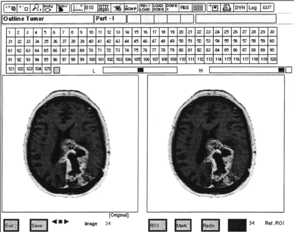
After the Gd+ files have been opened in MacNCTPlan, the tumor localization (outlining) is directed by the physician. For each slice, the tumor is defined (outlined) by drawing a line around it. This line defines a region of interest, or ROI. When all of the tumor has been outlined, the ROI is saved in a separate file to be used with the I- stack. When this step is completed, the I- stack is opened and used for the remaining

MacNCTPlan Part I procedures. The screen shot of MacNCTPlan in figure 2.6 shows the tumor localization.

!' 13r'

II ~ I '1 : 1 I,! I I o E 1 r I E I I k I DYH ILog I lEXrI

Outline Tumor Pat-I

I

ZI

1 2 3 4 15 6 7 8 9 10 11 12 13 14 15 16 17 18 19 2D 21 22 23 3 23 2 5 26 29 30 31 32 33 34 353 37 38 39 40 41 42 43 44 45 46 47 48 49 o0 51 2 53 O 5 '% T7 1 OA 60 61 62 63 64 65 66 67 68 9 70 71 72 73 74 T5 76 7- 78 79 80 81 82 83 84 85 86 87 88 89 9D 91 93 9$ 95 97 96 99 100 101 1021 1031 1 105 171 108 109 1101111112 113 114 11 116 1 11 9 1D [Originel]

9Iknage

Figure 2.6 Screen Shot of MacNCTPlan Tumor Outlining

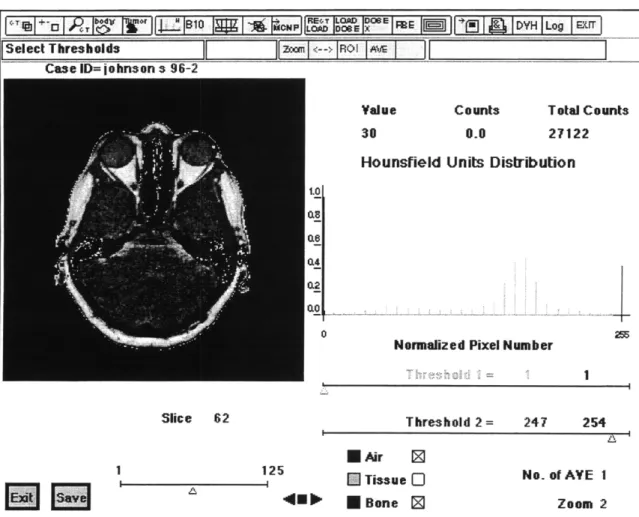
The next step within MacNCTPlan is to differentiate air, bone and soft tissue by thresholding the pixel intensities. Since the images were inverted, the air is colored white due to its low image intensities, while the bone is dark at high image intensities. MacNCTPlan allows the user to adjust the pixel intensity threshold for any slice and color the corresponding air, tissue or bone blue, green or red respectively. The coloration allows visual feedback as the threshold is changed. Figures 2.7 is a MacNCTPlan screen shot showing the thresholding step in MacNCTPlan. The reason that the I- stack is used now becomes obvious. The I+ stack, if thresholded, would contain bone in locations that it does not exist. The MRI stack does not lend itself to thresholding, since the bone and

air are similar in intensity. Even if the image is inverted and the air is artificially colored white, the thresholding problem is even worse than in the I+ stack.

., h*"PI LOAD DOE I DYH Lpg I .wr

Select Thresholds m rII--> ROI I

Case ID= jo hnson s 96-2

Value 30

Hounsfield

Counts Total Counts

0.0 27122

Units Distribution

0 2

Normalized Pixel Number

Threshold 2 = 247 254

Figure 2.7 Screen

1 125

Capture of MacNCTPlan Thresholding

* Air 0

E] Tissue O

E Bone I2

No. or AVE 1

Zoom 2

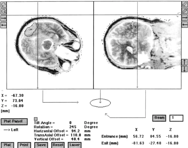
The next significant step after thresholding is the determination of irradiation beam orientations. The medical physicist uses his experience of dose distributions to determine three to five possible beams. Deep tumors usually receive a bilateral irradiation to increase dose to regions that would have low dose contributions from the first beam. To precisely define the exact entrance and exit locations of the beams, the stack is manipulated in three dimensions, allowing two cross hairs to be placed at the preferred entrance location. To guide the medical physicist, the irradiation beam's central axis and edges are displayed superimposed over the reconstructed CT images of two

orthogonal planes along the central beam axis. Figure 2.8 shows a screen capture of the beam direction portion of MacNCTPlan.

X= -67.30

Y = 73.64

Z = -16.00 [mm)

Tilt Angle = 0 Degree

Rotation = 245 Degree

-> Left Horizontal Offset= 94.2 mm X Y Z

TransAxialOffset= 110.0 mm Entrance (mm) 56.72 84.55 -16.00 Yertical Offset = 40.4 mm

V01 Exit [mm] -81.63 -27.48 -16.00

Figure 2.8 MacNCTPlan Screen Capture of Beam Positioning

The final important step is the creation of the head model, a 21 cm by 21 cm by 25 cm lattice of 1 cm3 _{cells. The CT data in each cell are represented as a certain}

percentage of soft tissue, tumor, bone and air, rounded to the nearest twenty percent. This averaging process uses nearby pixels in the same plane, as well as adjacent planes. After voxelization, each cell's location and composition is saved to a materials file. This file also includes the beam entrance and exit locations, thresholding values and anticipated boron concentrations for each beam set in previous portions of MacNCTPlan. Figure 2.9 shows a CT slice and its corresponding voxelized data.

Figure 2.9 MacNCTPlan CT Voxelization

2.2.3. MPREP

More information is needed to create an MCNP input deck. The FORTRAN 77 program MPREP incorporates the MacNCTPlan materials file with files containing other information necessary for MCNP. The spatial, angular and energy characteristics of the neutron and photon beams, as well as the kerma factors for each dose component are required. MPREP also prepares this information in the format required for the MCNP input deck, calculating the necessary surfaces, planes, and material fractions.

The MCNP materials themselves are each a different combination of air, bone, tumor and soft tissue. For example, MCNP material 11 is 20 % bone, 80% normal tissue, while MCNP material 32 is 20 % tumor, 40 % bone, 20 % normal tissue and 20% air. This material may appear in a cell containing the scalp and some surrounding air, the cranium and a portion of a tumor near the surface. There are fifty six combinations of materials, although not all of them are used in a given model.

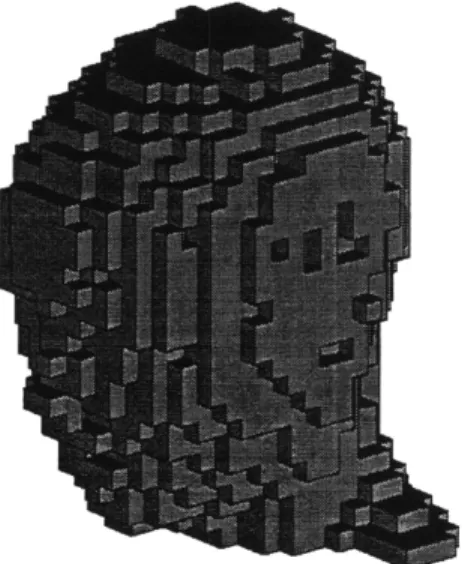
MPREP converts the cells into the appropriate lattice model. It can also represent the cells individually, without the lattice structure. Since MCNP cannot have photon and neutron sources in the same input deck, MPREP creates photon and neutron input decks for each beam. Figure 2.10 shows the head model of the non lattice version. The visualization program Sabrina cannot display lattices, although the picture would be

similar. The two versions, lattice and non lattice, have different memory requirements and run times, as described in sections 2.3.1 and 2.3.2.

Figure 2.10 Sabrina 3-D representation of the head model. The head is pointing to the left.

2.2.4. MCNP Calculations

After the neutron and photon input decks are created for each beam, MCNP uses them to calculate the dose rates for each voxel. A more detailed explanation of the input decks is given in chapter 3. Typically, one to three million particle histories are used to for scoping runs, which generate results with 5% statistical error in the region of interest. A description of this error and the number of particles used in scoping runs is given in

section 3.1.1.

2.2.5. MacNCTPlan Part II

After MCNP calculates the dose rates, the second part of MacNCTPlan is entered. The voxel dose rates for each beam are loaded into MacNCTPlan. From this information, MacNCTPlan interpolates the dose rate to each pixel using a 3D cubic spline. The dose rate data are then shown as isodose contours superimposed over the brain morphology. Tumor and normal tissue isodose rate contours are separately displayed superimposed over the entire brain. The medical physicist then compares the therapeutic ratio of the

minimum tumor dose rate to the maximum normal tissue dose rate, assuming some average boron concentration for each.

The maximum and minimum ratio of tumor dose rate to maximum normal tissue dose rate is then determined for various beam orientations. Using MacNCTPlan, various slices of the tumor are viewed and the appropriate dose rate is recorded. MacNCTPlan can calculate this ratio when the user specifies the normalization factor to be the healthy tissue maximum dose rate, so isoratio contours are plotted. Both visualization techniques allow the medical physicist to obtain an understanding of the volumes encircled by a particular threshold. With the current MIT epithermal neutron beam, the maximum therapeutic ratio is on the order of three or four. The minimum depends heavily on tumor location, and can be less than one for deep tumors.

In cases where the tumor is located near the eyes or optic chiasm, the dose rate to these radiation sensitive structures is determined. If a dual beam irradiation is being considered, the dose distributions from both beams are assessed. To calculate the dose to a sensitive structure, it is assumed that the maximum dose rate location will receive the prescription dose. The prescription dose can then be divided by the ratio of the dose rates to the sensitive structure and the maximum tissue location to determine the absolute dose to these locations. If the dose is unacceptably high, another beam orientation or weighting is selected. The dose to parotid glands, a sensitive structure as reported by Brookhaven National Laboratory (BNL), is also occasionally evaluated if they are in high dose rate locations. To lower the dose to these structures, a posterior beam entry was used.

Although MacNCTPlan gives the medical physicist absolute control over where to place the beams, the actual physical setup used will be limited by the range of the subject positioning device (couch) and the subject's tolerance of discomfort and his or her flexibility. Typical limitations are around twelve degrees lateral tilt of the positioning device, combined with the subject's physical ability to turn his or her neck. For example, irradiation beams cannot be directed into the center of the back of the head in a transverse

plane because the subject cannot be placed face down, nor would it be optimal for the beam to pass throughout the positioning device's headrest.

Occasionally, the medical physicist determines that a small dose to the deep portions of a tumor from a beam entering the contralateral side of the subject's head will yield the best therapeutic ratio. This effect can be accounted for by adjusting a fluence weighting factor. It is the ratio of neutron fluence in the second beam to that of the first. Since the neutron fluence rates may vary slightly, this ratio is not strictly the ratio of the length of irradiations, but is often considered as such.

The physician will occasionally be interested in the use of dose volume histograms (DVH). These can be generated within MacNCTPlan or calculated in an Excel spreadsheet directly from the MCNP data (see section 5.1). In MacNCTPlan Part II, the tumor ROIs can be used as a guide to determine the volume of interest, or the brain tissue or a sensitive structure volume can be outlined and defined as the new ROI. MacNCTPlan will automatically calculate the volume identified, and the relative volume containing a certain dose rate or higher. Below is a screen shot of MacNCTPlan's dose rate volume histogram (DRVH) generation ability. Since the effects of different °B concentrations and irradiation times can be included, these DRVHs will show an identical shape as the DVH.

After the final beam selection has been made, each final beam calculation is run for ten million source particles, which results in one or two percent error of total dose to the tumor region. This calculation typically requires a run time of fourteen hours on a 200 MHz Pentium Pro computer.

2.3 Monte Carlo N Particle Radiation Transport Code (MCNP)

Determining dose rates to locations in the subject is an integral part of BNCT treatment planning. The Monte Carlo radiation transport code, MCNP, is the integral part of calculating the dose rates. MCNP, a well tested and documented code developed by Los Alamos National Laboratory (LANL), is successful at simulating the complexities of the irradiation. As mentioned before, it is capable of representing the subject's head, the

energy, angular, and radial distributions of the neutrons and gammas emitted from the MITR-II Medical room's epithermal neutron beam. Since the beam contains thermal, epithermal and fast neutron components, MCNP's detailed transport calculations are used to calculate the thermalization and subsequent dose of neutrons through elastic and inelastic collisions with varying isotopes, in addition to the photons created by neutron absorption. When elevated concentrations of 'OB are present in the model, MCNP calculates the amount of flux depression and the corresponding change in the dose distribution. MCNP does not track the radiations from the delayed decay of radioisotopes, nor does MCNP include photoneutron creation.

MCNP uses an input file, or input deck, that completely describes the model of the problem that the user wants to simulate. Everything from source characteristics to output format is controlled through this input deck. Significant components of a deck used for BNCT treatment planing are the geometric patient model, either lattice or non lattice based, materials entries, source description, kerma factors and tallies. Each of these is described in detail in this chapter. For a more complete description of input deck options, the reader should refer to the MCNP 4B Manual 2.

2.3.1 Lattice Model

The lattice model of MCNP is a geometric structure: a grid of regular hexahedra, either cubes or triangular prisms. The grid is formed by an infinitely repeating array of regularly spaced planes. A contiguous region of space bounded by these planes is a

single lattice element. Since each lattice element can contain several objects, including other nested lattices, a system of layers, or universes, is used to fully describe the model. A universe is a region of infinite space.

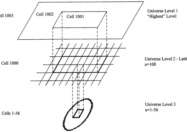
The universe structure for the BNCT patient modeling involves three levels, as illustrated in two dimensions in Fig 2.11.

Cell 1003 ell 1002 Cell 1001 Cell 1000 I/ I I II I I II I I I I I Universe Level 1 "Highest" Level

Universe Level 2 -Lattice u=100

Universe Level 3 u=1-56

Cells 1-56

Figure 2.11 Illustration of Multiple Universe Levels. shown, each lattice element has a corresponding cell.

Although only one cell in universe level three is

The root universe, or "highest" level, contains the "window" (cell 1001) looking onto the lattice level. Since the lattice is an infinitely repeating structure, it is this "window" which defines how much of the lattice will be visible in the root level, or used for transport. The window is filled with universe 100, which is a cubic lattice (cell 1000). Each lattice element is filled with a lower level universe. This third and lowest level contains cells (cells 1-56) with specified material properties. Just as in the lattice cell, only the portion of these cells that corresponds to the movement of the particle through the lattice element will actually be used. The other two cells in the root level, cell 1002

and 1003, define everywhere external to this window. Cell 1002 is the region of air surrounding the 21 cm by 21 cm by 25 cm model where neutron and photon transport is important. Cell 1003 is a sphere beyond which no transport occurs. Particles passing into cell 1003 are terminated.

The portion of the Harvard/MIT BNCT treatment planning input deck describing the above model is shown in figure 2.12.

c cell cards

c

1000 0 -112 111 -212 211 -312 311

lat=l fill= 0: 20 0: 20 0: 24

56 56 56 56 56 56 56 56 56 56 26 26 26 26 1 26 56 56 56 56 56 56

[many more lines of data]

56 56 56 56 56 56 56 56 56 56 56 56 56 56 56 56 56 56 56 56 56 56 u=100

1 1 -1.04700E+00 -70 u= 1

[all other universe material cards]

56 56 -1.29300E-03 -70 u= 56 1001 0 111 -113 211 -213 311 -313 fill=100 $ Window 1002 0 -1000 ( -111: 113: -211: 213: -311: 313) $ Outside Window 1003 0 1000 $ No Transport Beyond Here c BLANK LINE c BLANK LINE c c surface cards

111 px -10.500000 $ Set of Planes in X direction

112 px -9.500000

113 px 10.500000

211 py -10.500000 $ Set of Planes in X direction

212 py -9.500000

213 py 10.500000

311 pz -10.500000 $ Set of Planes in X direction

312 pz -9.500000

313 pz 10.500000

1000 so 5.56417E+01

70 so 5.56417E+01

c

Figure 2.12 MCNP Lattice cells and surfaces.

In this example, cell 1000, the lattice, has material zero (i.e. void), and is bounded

by the planes 112, 111, etc. These planes form a single 1 cm3 _{voxel. Although this voxel}

is repeated infinitely in the three Cartesian directions, the window bounded by planes

that the center voxel of the entire 21 cm by 21 cm by 25 cm matrix of voxels is at the coordinate (0, 0, 0). The order of the listed planes is important in defining the indices and in what direction they increase. Since 112 is listed first, the voxel in the same y, z location but at -9.0 would be [1,0,0]. The lat=l option specifies that the lattice is filled with hexahedra, while lat=-2 would fill the lattice with hexagonal prisms. The fill option specifies the number of the universe in the next lower level. The listing of fifty-six different universes for each of the 11025 lattice elements specifies which universe each lattice element is filled by. After the lattice cell entry is a listing of fifty-six cells, each specifying a density and material, 1 through 56, belonging to their corresponding universe listed on the lattice card. These cells, although they could be cubes or any other shape that defines the bounding surfaces of a cell, are spheres for simplicity.

After the cell listings is a blank line followed by the surface listings. These surface cards describe planes and spheres that bound the lattice and the regions of importance. This input file uses the new ability of MCNP4B to have coincident window and lattice bounding planes, previously a small offset was required Although not shown above, the imp card sets the importance of every cell to 1, except cell 1003, the external world, which is set to zero.

2.3.2 Non Lattice Model

The standard cell geometry of MCNP fully describes the location, material, and boundaries of each of the 11025 cells, without using lattices or multiple universe levels. Figure 2.13 shows a portion of the input deck where all planes and cells are listed explicitly.

c cell cards

c

1 56 -0.12930E-02 11i

2 56 -0.12930E-02 112

3 56 -0.12930E-02 113

[many cell cards]

11025 56 -0.12930E-02 131 11026 0 -1000 ( -111: 11027 0 1000 c BLANK LINE c BLANK LINE c 111 px -10.500000 112 px -9.500000 113 px -8.500000 114 px -7.500000 115 px -6.500000

[many other px, py, pz planes]

Figure 2.13 MCNP non-lattice cells and surfaces.

-112 -113 -114 211 -212 211 -212 211 -212 311 -312 311 -312 311 -312 -132 231 -232 335 -336 132: -211: 232: -311: 336)

The non lattice neutron and gamma BNCT problems require six and forty-three Megabytes of RAM, respectively. These memory requirements are large enough to prevent MCNP from operating within a Windows NT DOS window. The standard MCNP4B lattice version decreases these memory requirements to nineteen and fourteen Mbytes, but it prohibitively increases wall clock runtimes, by a factor of about one hundred. The non lattice model capability is useful to retain for running on other platforms, such as UNIX, especially when MCNP cannot be recompiled with time reducing enhancements, and for model visualization with Sabrina. During the Harvard/MIT treatment planning calculations, the lattice model is used exclusively.

2.3.3

MCNP Materials

MCNP requires a description of the matter that fills any location. The materials card provides a description of the isotopes and abundances, as well as the cross section library associated with each isotope. Figure 2.14 is a part of the materials portion of the input deck.

ml 1001.50c -0.1058481 6012.50c -0.1395953 7014.50c 8016.50c -0.7269170 15031.50c -0.0039055 17000.50c 19000.50c -0.0039055 5010.50c -0.0000010 m2 1001.50c -0.1058481 6012.50c -0.1395953 7014.50c 8016.50c -0.7269168 15031.50c -0.0039055 17000.50c 19000.50c -0.0039055 5010.50c -0.0000012 m3 1001.50c -0.1058480 6012.50c -0.1395952 7014.50c 8016.50c -0.7269167 15031.50c -0.0039055 17000.50c 19000.50c -0.0039055 5010.50c -0.0000014 [portion removed] m52 1001.50c -0.0499354 6012.50c -0.1398192 7014.50c 8016.50c -0.4497058 15031.50c -0.1098579 20000.50c m53 1001.50c -0.1053278 6012.50c -0.1389091 7014.50c 8016.50c -0.7244360 15031.50c -0.0038863 17000.50c 19000.50c -0.0038863 5010.50c -0.0000010 m54 1001.50c -0.1053277 6012.50c -0.1389090 7014.50c 8016.50c -0.7244353 15031.50c -0.0038863 17000.50c 19000.50c -0.0038863 5010.50c -0.0000020 m55 1001.50c -0.0498282 6012.50c -0.1395189 7014.50c 8016.50c -0.4492173 15031.50c -0.1096220 20000.50c m56 7014.50c -0.7778000 8016.50c -0.2222000 -0.0184258 -0.0014020 -0.0184258 -0.0014020 -0.0184258 -0.0014020 -0.0409527 -0.2097288 -0.0221585 -0.0013951 -0.0221585 -0.0013951 -0.0425352 -0.2092784

Figure 2.14 Materials Cards in MCNP BNCT treatment planning input deck.

The ml states that for material one, an isotope with atomic number of one and

atomic mass of 001, i.e. 'H, is present with a mass fraction of 0.1058481, an isotope with an atomic number of 6 and atomic mass of 012, i.e. 12C, is present with a mass

abundance of 0.1395953, etc. The ".50c" after each isotope identification indicates that the continuous cross sectional data from the Evaluated Nuclear Data File (ENDF) V library data set, should be used. The minus sign indicates the mass fraction rather than atomic fraction is used. Densities are specified in the cell cards.

As indicated in Chapter two, each of these materials corresponds to a different fractional combination of air, tissue, bone and tumor or other ROI defined region of space. Table 3.1 lists the combination of these in each material.

Table 3.1 MCNP Material Composition Fractions

AIR BONE NORMAL TISSUE TUMOR MCNP Material

0 0 0 100 1 0 0 20 80 2 0 0 40 60 3 0 0 60 40 4 0 0 80 20 5 0 0 100 0 6 0 20 0 80 7 0 20 20 60 8 0 20 40 40 9 0 20 60 20 10 0 20 80 0 11 0 40 0 60 12 0 40 20 40 13 0 40 40 20 14 0 40 60 0 15 0 60 0 40 16 0 60 20 20 17 0 60 40 0 18 0 80 0 20 19 0 80 20 0 20 0 100 0 0 21 20 0 0 80 22 20 0 20 60 23 20 0 40 40 24 20 0 60 20 25 20 0 80 0 26 20 20 0 60 27 20 20 20 40 28 20 20 40 20 29 20 20 60 0 30 20 40 0 40 31 20 40 20 20 32 20 40 40 0 33 20 60 0 20 34 20 60 20 0 35 20 80 0 0 36 40 0 0 60 37 40 0 20 40 38 40 0 40 20 39 40 0 60 0 40 40 20 0 40 41 40 20 20 20 42 40 20 40 0 43 40 40 0 20 44 40 40 20 0 45 40 60 0 0 46 60 0 0 40 47 60 0 20 20 48 60 0 40 0 49 60 20 0 20 50 60 20 20 0 51 60 40 0 0 52 80 0 0 20 53 80 0 20 0 54 80 20 0 0 55 100 0 0 0 56

Although there are fifty six materials listed, not all of them are significantly different. The difference between materials three and four, one sixty percent tumor forty