An automated matching algorithm for dual orthogonal fluoroscopy

An Automated Matching Algorithm for Dual

Orthogonal Fluoroscopy

by

Jeffrey Thomas Bingham

Submitted to the Department of Mechanical Engineering

in partial fulfillment of the requirements for the degree of

Master of Science in Mechanical Engineering

at the

MASSACHUSETTS INSTITUTE OF TECHNOLOGY

June 2006

@

Massachusetts Institute of Technology 2006. All rights reserved.

A uthor ... ..

...

Department of Mechanical Engineering

May 12, 2006

Certified by..

Guoan Li

(72

Associate Professor of Orthopaedic Surgery

Harvard Medical School

Thesis Supervisor

Certified by..

Derek Rowell

A

Professor of Mechanical Engineering

Thesis Supervisor

A ccepted by .... ... 4r ... ...

MASSAHU S INTITir=E

Cha

Lallit Anand

Professor of Mechanical Engineering

irman, Committee on Graduate Students

An Automated Matching Algorithm for Dual Orthogonal

Fluoroscopy

by

Jeffrey Thomas Bingham

Submitted to the Department of Mechanical Engineering on May 12, 2006, in partial fulfillment of the

requirements for the degree of

Master of Science in Mechanical Engineering

Abstract

The current method of studying in vivo kinematics of human joints is a tedious and time consuming task. Current techniques require the segmentation of hundreds of raster images, often by hand, and registration of three-dimensional models with two-dimensional contours. Automation of these processes would greatly accelerate research in this field. This research presents an automated method for recovering the pose of a three dimensional model from planar contours. Validation of the algorithm and discussion of its performance and applicability are detailed herein.

Thesis Supervisor: Guoan Li

Title: Associate Professor of Orthopaedic Surgery Harvard Medical School

Thesis Supervisor: Derek Rowell

Acknowledgments

With the opportunity to point fingers at people who made me the way I am, I jump at the chance to accuse my benefactors. First and foremost I thank my mother and father. My successes have been achieved through the love, inspiration, knowledge,

and guidance they have given me. My family, especially my little sister, has made life worth living.

I must also acknowledge the many teachers and mentors of my life, who have shown me the secrets of engineering. Mr. Walker, who taught me what an engineer should be; Prof. Schoen, who introduced me to research; and Dr. Li, who enabled this research.

Finally, I thank my friends in Idaho and MIT. Remembering all of the fun times, helped muscle through the rough spots. Besides, I like to think that together we conquer the world.

In short, I am very thankful for the opportunity to write this thesis. My life has been truly blessed because of the people in my life, without them I am nothing.

".... because I am involved in mankind, and therefore never send to know for whom

Contents

2 Pose Reconstruction Procedure 23 2.1 Imaging . . . . 23 2.1.1 MRI . . . . 25 2.1.2 Dual-Orthogonal Fluoroscopy . . . . 25 2.2 Image Analysis . . . . 26 2.2.1 Distortion Correction . . . . 26 2.2.2 Segmentation . . . . 27 2.2.3 Environment Recreation . . . . 29 2.3 Matching . . . . 30 3 Automated Matching 33 3.1 Objective Function . . . . 34 3.1.1 Transformation . . . . 34 3.1.2 Projection . . . . 35 3.1.3 Point Selection . . . . 35

3.1.4 Error Computation . . . . 36

3.2 Optimization . . . . 37

3.3 Summary . . . . 39

4 Validation and Application 41 4.1 Idealized Environments . . . . 41

4.1.1 TKA Components . . . . 42

4.1.2 Natural Knee . . . . 44

4.2 Standardized In-vitro Environments . . . . 46

4.2.1 Spheres . . . . 46 4.2.2 Natural Knee . . . . 48 4.3 In-vivo Environments . . . . 49 4.3.1 TKA Components . . . . 49 4.4 Summary . . . . 51 5 Discussion 53 5.1 Algorithm Operation . . . . 53

5.2 Comparison with Previous Algorithms . . . . 55

5.3 Single vs. Dual Fluoroscopy . . . . 58

5.4 Future Work . . . . 62

A Matlab Source Code 65 A.1 Environment Setup . . . . 66

A.1.1 correctlmage.m . . . . 67

A.1.2 assembleMesh.m . . . . 68

A.2 Automatic Matching . . . . 70

A.2.1 FINDPOSE.m . . . . 71

List of Figures

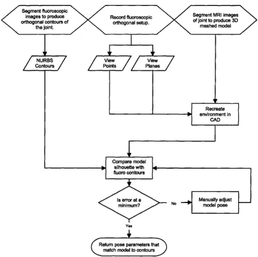
2-1 Flow of the manual matching process... 24

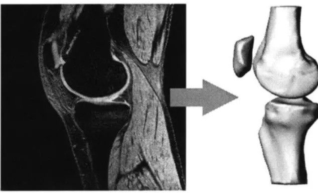
2-2 Example of MRI model construction . . . . 25

2-3 Dual-orthogonal fluoroscopic system . . . . 26

2-4 Canny automatic segmentation of a fluoroscopic image. . . . . 28

2-5 Virtual dual-orthogonal fluoroscopic system . . . . 29

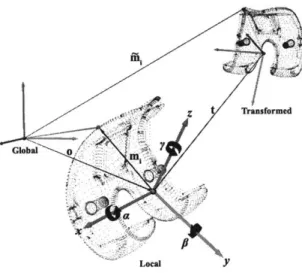
2-6 Local and global coordinate systems for matching . . . . 30

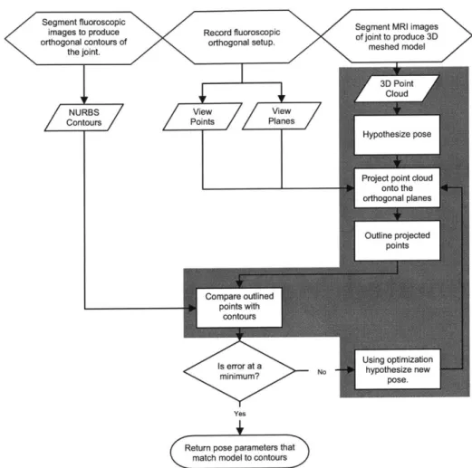
3-1 Flow of the automated matching process . . . . 34

3-2 Outlining procedure . . . . 36

3-3 Calculating error in matching projections . . . . 37

4-1 A virtual environment for the standardized in-vitro sphere test. . . . 46

4-2 Geometry of standardized sphere test . . . . 47

4-3 A virtual environment for an in-vivo TKA test. . . . . 50

5-1 Schematic of in-plane vs. out-of-plane error . . . . 59

List of Tables

4.1 Size effects on ideal TKA geometry . . . . 43

4.2 Pose effects on ideal TKA geometry . . . . 44

4.3 Pose effects on ideal knee geometry . . . . 45

4.4 Error in matching sphere geometry . . . . 47

4.5 Error in matching in-vitro knee geometry . . . . 49

4.6 In-vivo repeatability of matching TKA geometry . . . . 51

5.1 Algorithm comparison with simulated data. . . . . 56

5.2 Algorithm comparison with in-vivo TKA data. . . . . 57

5.3 Effect of single vs. dual plane data on automatic matching . . . . 60

5.4 Effect of geometry on single vs. dual plane data . . . . 61

Chapter 1

Introduction

Fluoroscopic imaging techniques have been used extensively to measure in-vivo kine-matics of total knee arthroplasty (TKA) because of the relatively low radiation dosage and the accessibility of the equipment [2, 9, 25]. Previous studies employed a sin-gle fluoroscope to take sagittal plane images of the knee at multiple flexion ansin-gles [2, 10, 29, 6, 32]. Using the geometry of the fluoroscope, three dimensional (3D) computer models of the tibial and femoral components were matched to the two-dimensional (2D) features of the acquired fluoroscopic images. When the features were considered to be matched, the relative poses of the 3D component models rep-resented the in-vivo knee kinematics, where pose is defined as the position and orien-tation specifying the six degree-of-freedom (6DOF) location of an object. Using this technique numerous data have been reported on knee motion within the image plane of the fluoroscope. However, determining knee motion in the direction perpendicular to the fluoroscopic image plane has been questioned in recent studies [31, 15, 19].

Pursuing higher accuracies with fluoroscopy, Li et al. [19] completed a 3D study on quasi-dynamic in-vivo kinematics of the knee and more recently, Hanson et al. [9] and Suggs et al.[26] applied two fluoroscopes to formulate a dual-orthogonal fluoroscopic system to investigate in-vivo TKA kinematics. These studies utilized a computer aided drafting (CAD) program to simulate the fluoroscopic environment and manually manipulate 3D models in space so that their projected silhouettes matched outlines of the components on both fluoroscopic images. This methodology has been proven

to accurately recreate the 6DOF motion of the knee at multiple flexion angles [9].

However, the manual matching procedure is laborious, impairing its application to study continuous dynamic motion. Automating the matching procedure would reduce the time required to match and improve the repeatability of the dual fluoroscope methodology in determining in-vivo kinematics.

An optimization algorithm is presented for automating the process of matching projections of 3D models of the tibia and femur to two orthogonal planar images of the patient acquired with a dual-orthogonal fluoroscopic imaging system. Accuracy and repeatability of the algorithm's ability to determine 6DOF location are discussed. Results from a complete validation demonstrate the repeatability of the algorithm for determining in-vivo TKA poses.

1.1

Previous Methods

Current research on recreating the pose of 3D objects in the orthopaedic field is driven mostly by the desire to determine joint kinematics. Pose reconstruction from radiographic data offers a non-invasive method for examining in vivo motion of joints. The method itself is conceptually simple. A computer generated three-dimensional model of the joint is obtained through MRI or CT imaging, and then radiographs are taken with the joint in motion. The next step is to match a pose of the three-dimensional computer model to the radiographs of the joint motion. This effectively gives one a three-dimensional dynamic model of the joint in question.

The three main methods requiring pose reconstruction include stereophotogram-metry, single plane fluoroscopy and biplanar fluoroscopy. Each method uses either a variation of the hypothesis and test algorithm or a template matching scheme to determine the true pose of the model. Variations of the hypothesis and test algorithm include iterative closest point, non-overlapping area, iterative inverse point matching and image matching of digitally reconstructed radiographs. These variations provide a method of formulating an objective function which is then optimized using a wide range of available minimization routines.

1.1.1

Imaging Methodology

The first classification of these pose recreation methods lies in the imaging techniques. Three dimensional imaging is used to generate very accurate anatomical models of patient geometry. Two dimensional imaging allows for acquisition of high speed motion of a patient performing functional activities, which provides a record of the in-vivo kinematics. The combination of the 2D and 3D data is then used to generate a database of highly accurate six degree-of-freedom kinematics. Several different methods of acquiring this data has been presented in the literature.

Three Dimensional Imaging

The creation of the three dimensional model is done with a variety of techniques depending on the application. For in-vivo models the majority are created by seg-menting images from MRI and creating solid mesh models. A small number of re-searchers have also used CT scan data to create these models. Combined CT and MRI data have also been used to create voxel models as well. For patients who have had arthroplasty, models from manufacturer CAD and laser scanning of the components has been employed.

Two Dimensional Imaging

The creation of radiographs for pose recreation has been accomplished with x-ray and fluoroscopy. Fluoroscopy is distinguished from x-ray by having a lower radiation dose, which is accomplished by employing a fluorescent detector. Image quality is generally better with high dosage x-ray, but the hazard to the patient makes fluoroscopy a more desirable method. However, the greatest effect on pose recreation is the number and geometry of simultaneous radiographic images taken. Radiographic configurations currently in practice include roentgen stereophotogrammetry (RSA), single plane flu-oroscopy and biplanar fluflu-oroscopy. RSA is the oldest method and was originally accomplished by implanting radio-opaque markers into the patient, but has recently employed markerless techniques[7, 27, 28]. RSA takes two simultaneous images from

separate focal points, which are projected onto a single plane. Fluoroscopy, on the other-hand, has two variants. The majority of the past research has used a single fluoroscopic image plane[2, 6, 10, 11, 15, 20, 21, 29, 30, 32]. Recently researchers have employed two fluoroscopic images, some in orthographic configurations, and others in more conventional stereo modes[1, 4, 9, 16, 19, 18, 26, 31].

1.1.2

Algorithm Type

Pose recreation can be further classified based on the algorithms used for determining pose. Most of these algorithms have their origins in machine vision algorithms and computer graphics. In general they have been modified to meet the particular

re-quirements of the pose recreation problem. In general there are only two algorithms,

template matching and hypothesis and test.

Template Matching

Template matching for pose recreation in biomechanics was pioneered by Banks and Hoff[2, 10]. In template matching the 3D model is first segmented into a library of many different projections. Each library record contains a silhouette of the projected model and the corresponding pose variables. Then by implementing shape matching techniques, outlines in the library are matched to contours segmented from fluoro-scopic contours. Libraries of outlines have been created using silhouettes normalized for rotation, translation and scale. This can be done directly or by parameterizing the contours with fourier coefficients. Similarity values are computed based on similarity of normalized parameters or total amount of overlapping area.

Hypothesis and Test

Hypothesis and test is a very generic structure of pose estimation. The algorithm consists simply of two parts, determining a "hypothesis" for the position of the ideal pose and applying a "test" to determine the validity of the hypothesis[14]. In practice the variations of the algorithm are best characterized by their methods of

optimiza-tion and their formulaoptimiza-tion of objective funcoptimiza-tions. Optimizaoptimiza-tion being the method of determining a successively better hypothesis and the objective function a method of testing validity and guiding the next hypothesis of pose.

1.1.3

Optimization

Due to the highly non-linear nature of any feasible objective function employed to determine pose, the optimization methods used to date are either nonlinear global algorithms or heuristic direct search methods. Classical gradient methods that have been employed include: Levenberg-Marquardt Least Squares, and Feasible Sequen-tial Quadratic Programming. Heuristic direct search methods include: Simulated Annealing, Sequential Parameter Search and Powell's Method. Brief description of these methods and several other suggested minimization routines are given below.

Levenberg-Marquardt Nonlinear Least Squares

This method was first used by Lavallee and later Zuffi and Yamazaki[16, 32, 30]. The method utilizes a trust region modification of the Gauss Newton algorithm, this optimization method switches between gradient descent and Gauss-Newton for best trade-off of speed and convergence.

Feasible Sequential Quadratic Programming

This is a further advancement of the Gauss-Newton scheme, and assumes the problem is in quadratic form and all constraints are linearized. Feasible refers to only allowing values of the dependent variables within a desired or computable range. Kanisawa, Kaptein and Valstar have used this method of optimization[11, 13, 28].

Nelder-Mead Downhill Simplex Method

Yamazaki also introduced this method for finding the optimal pose[30]. A simplex is the term given to a "figure" which has n+1 vertices in the n-dimensional search space. The simplex is used for determining search directions and is continually expanded,

contracted or reflected based on minimization of the vertices. Random steps are interjected to help remove difficulties with local minima.

Powell's Method

Powell's method presents an optimization algorithm that does not require finding the partial derivatives. It increments along a set of conjugate base vectors in order to find a minimum. Simply put the algorithm starts with a set of initial vectors, computes a function step and based on the results of the step re-computes the solution vectors. This is repeated until a minimum is found. Tomazevic used Powell's Method for minimization[27].

Simulated Annealing

A popular heurestic method for solving global optimization problems and used by

several authors [20, 31]. A search space is defined, a random generator modifies the search variables based on a "temperature" and at each iteration the temperature is "cooled" lowering the change in variables. The cooling schedule is predefined with rules for when to change the step sizes.

Sequential Parameter Search

A very straightforward method utilized by Hoff[10]. Each variable in the search space

is sequentially minimized. Variations of this also introduce curve fitting techniques in order to determine minimum basis directions that do not directly follow a single parameter.

Swarming

A more recent heurestic search method of swarming was investigated by Schutte[23].

Random points in the search space are computed, the random cloud of search points then moves towards the minimum point with the greatest "velocity". Based on the total velocity of the cloud, these points move through the search space, until a global minimum is reached.

1.1.4

Objective Functions

The bulk of any variation of the hypothesis and test algorithm lies in defining a procedure that will test the validity of a given pose and help to determine the next best guess. This procedure is termed an objective function, cost function and sometimes performance index in literature. In this paper it is referred to as an objective function. Its purpose is to define a function which returns a scalar quantity that when minimized results in an ideal match of the model pose from the given silhouette data.

Iterative Closest Point

The Iterative Closest Point (ICP) algorithm minimizes the distance between points on the projected contour and the given contour[6, 12]. The distance compared is the minimum distance for each point to the given contour, hence the name. When this distance is minimized the projected contour should be exactly the given contour and the pose found.

Non-overlapping Area

Non-overlapping Area (NOA) is also well described by its name[28]. After projecting a silhouette from the model, any area that is not simultaneously covered by both the projected and given silhouettes is summed. The NOA is then the union minus the intersection of the projected and given silhouettes. When this area is minimized the projected silhouette should perfectly overlay the given silhouette and the ideal pose is recovered.

Iterative Inverse Point

In the Iterative Inverse Point (IIP) matching algorithm, rays connecting the focal

point to points on the given contour are constructed. Then, distance between the model surface and the projected rays is minimized. When the rays form bi-tangents on the model's surface the ideal pose is recovered. Pre-computed maps describing the distance from the surface of the model have been used to reduce computational

burden. These three dimensional distance maps are constructed using a specialized quad-tree decomposition first implemented by Lavallee and later adopted by others[13,

16, 30, 32].

Digitally Reconstructed Radiographs

The algorithm for Digitally Reconstructed Radiograph (DRR) matching utilizes

ren-dering techniques in order to produce a projected raster image that simulates an x-ray[20, 27, 30]. The simulated raster image is then compared to the given x-ray

image. When similarity between the two raster images is maximized the ideal pose is recovered. Image similarity measures for the raster images are accomplished using a variety of techniques used in image matching. Intensity values and edge overlap are the most widely used metrics. However, quad-tree decomposition and cross correla-tion have also been used successfully as measures of image similarity.

1.2

Motivation

Many factors affect the ability to recover the correct pose of a particular scene; how-ever, the number of simultaneous radiographic views has the greatest impact. This is because sensitivity of matching out-of-plane translation is far worse than translation within the plane. In order to minimize error a procedure using two orthogonal radio-graphs has been developed that combines the best attributes of magnetic resonance imaging (MRI) and fluoroscopy[4, 9, 19].

This imaging procedure can be applied to most of the articulating joints in the human body. This allows for highly accurate in-vivo study of joint kinematics and dynamics, cartilage contact and ligament interaction. The technique is especially attractive for accurate measurement of in vivo kinematics of patients with orthopaedic implants because the 3D wire-frame model of the orthoses can be obtained directly from the CAD model used for manufacturing. Information gained from this imaging technique can be used for designing new medical devices, for pathological diagnosis and for planning surgical procedures as well.

Currently this procedure is accomplished manually, which is time consuming. Also, because of the vagaries of human precision, overall consistency is not well de-fined. Finally, the procedure necessitates the mastery of new knowledge and skills to achieve accurate results. A fully automated procedure will accelerate the match-ing process, stabilize repeatability and reduce the learnmatch-ing curve for the procedure. Research of algorithm development, algorithm implementation and validation of the procedure will ultimately realize a fully automated pose reconstruction. The purpose of this research is to present a method for automating this procedure and providing a thorough validation.

Chapter 2

Pose Reconstruction Procedure

The method of pose reconstruction is conceptually simple. A computer generated

3D model is obtained and radiographs are taken of the subject in motion. Based

on the geometry of the radiographic setup it is possible to match 2D features in the radiograph to points on the 3D model. When the features are matched the pose of the

3D model is recreated, which effectively gives one a 3D dynamic model. The process of

acquiring images with the dual-orthogonal fluoroscopic image system and recreating in-vivo kinematics can be separated into three stages: imaging, image analysis and matching. A flow chart of the manual process is shown in Fig. 2-1. Automating each of these tasks increases the speed of the system and improves the repeatability; however, this comes at a cost of lost sensitivity. When a balance between automation and manual interaction is reached the system is efficient, robust and accurate. To emphasize this balance, a discussion of the amount of human intervention accompanies the description of each stage of the process. These algorithms are implemented in Matlab software and listings can be found in Appendix A.

2.1

Imaging

Acquisition of the images is where the actual kinematic data is recorded. With the technological advancements in magnetic resonance imaging (MRI) and x-ray machines it is possible to recreate fully 3D anatomical models and also record human

activ-Segment fluoroscopic

images to produce Record fluoroscopic Segment MRI images

orthogonal ntours of orthogonal setup. of joint to produce 3D

othert3D reostutontciqenuing copuerai ed den(A)mdl

NURBS View View

Contours e , Points P aene s

Recreate kenvironment in CAD Compare model } silhouette with fluoro contours

Is error at a Manually adjust I

minimum? No model pose

Yes

Figure 2-1: Flow of the manual matching process.

ity in real-time. MRI provides a tool to recreate thee anatomy with sub-millimeter

precision. MRI can easily be replaced with computed tomography (CT) scans, or other 3D reconstruction techniques, including computer aided design (CAD) models of metal components; however, MRI is most often the least invasive method available.

Similarly, any x-ray method can be used, but pulsed fluoroscopy exposes the patient

to the least amount of radiation. The general imaging requirements of the process are therefore a method of recreating the 3D geometry and the ability to capture two

orthogonal images of the 3D geometry's motion. This research explored MRI and

CAD for model generation and pulsed fluoroscopy for acquiring images of patient

2.1.1 MRI

In order to create 3D models of living anatomy MRI has been utilized to capture the structure. For the knee joint, patients are asked to lie supine in an MRI having a

3 Tesla magnet. Using a knee coil, approximately 120 sagittal images are acquired

with a section thickness of 1 mm, a field of view of 160 x 160 mm and a resolution of 512 x 512 pixels. Acquisition was accomplished with a flip angle of 25', imaging frequency of 123.3 kHz, an echo time of 6.5 ms, and a 24 ms repetition time (Fig. 2-2).

Figure 2-2: An example MRI slice on the left used to construct the 3D surface model on the right.

2.1.2

Dual-Orthogonal Fluoroscopy

The dual-orthogonal fluoroscopic image system consists of two fluoroscopes (OEC

9800 ESP, GE, Salt Lake City) positioned with the two image intensifiers

perpendic-ular to each other (Fig. 2-3) [9]. A subject is free to move within the common imaging zone of the two fluoroscopes. The subject is then asked to move through a series of flexion angles which are imaged simultaneously by the fluoroscopes to acquire images of the knee from two perpendicular directions. During this procedure, the average subject receives 106 mrem of radiation for 20 seconds of pulsed fluoroscopy at 65

kVp and 0.80 mA. In addition to the subject images, a set of calibration images are

acquired. Calibration images are taken of a perforated plate for distortion correction and a set of beads in a known configuration for the recreation of the fluoroscopic

ge-ometry. The images are stored electronically with an 8-bit gray-scale and a resolution of 1024 x 1024 pixels, corresponding to a 315 x 315 mm field-of-view. This procedure records the in-vivo poses of the knee as a series of 2D paired orthogonal fluoroscopic

images.

Image Intensifiers

X-ray Sources

Figure 2-3: A dual-orthogonal fluoroscopic system for capturing in-vivo knee joint kinematics.

2.2

Image Analysis

In order to extract kinematic data from the acquired images the data must first be corrected for distortion, structural features then extracted and finally the fluoroscopic imaging system must be recreated in simulation. While each step can be automated, the entire process still requires a high level of human interaction. This is particu-larly true for segmentation, and without development of powerful machine learning algorithms, human operation will continue to provide the most efficient and reliable results.

2.2.1

Distortion Correction

The fluoroscopic images suffer from small amounts of distortion caused by the slightly curved surface of the image intensifier and environmental perturbations of the x-ray. In order to remove "swirl" caused by electro-magnetic disturbance and "fish-eye"

from the curved image surface a known grid is imaged and the subsequent image is mapped to the known geometry. A global surface mapping using a polynomial fitting technique adapted from Gronenschild is used to accomplish this [8]. Linear interpolation and local distortion correction were compared, but it was found that global correction provided the most consistent results.

A plexi-glass plate with a pattern of holes in concentric circles is used for the

reference geometry. This radial geometry was found to work best, because it conforms well with the circular intensifiers and allows for a high density grid that is conducive to solving the mapping problem. Distortion correction is accomplished by mapping the distorted grid to the known grid using a set of two-dimensional polynomials. The images themselves are corrected by using the spatial mapping to "move" pixels with linear interpolation of the intensity values. Matlab code used for correcting distorted images can be found in Appendix A.1.1.

2.2.2

Segmentation

Thresholding, region growing and edge detection have been explored as possible meth-ods of extracting structural information from raster images. In order to generate contours, edge detection is currently the most useful method. Most edge detection methods are variants of a basic premise of determining the maximum gradient of im-age intensity. Sobel, Prewitt, Roberts and Laplacian of Gaussian algorithms return similar results for fluoroscopic and MRI images. The most favorable algorithm is the one presented by Canny [3]. This algorithm improves on previous methods by adding rules for discarding erroneous edges. The basic algorithm first smooths the image using a Gaussian filter, then it computes the gradients from a Laplacian filter. Next, the gradients are reduced by removing non-maximal values. The edges created by the maximal values are further reduced by applying a threshold and examining con-nectivity. Non-maximal edges connected to maximal edges are kept, while isolated non-maximal edges are removed. Canny edge detection is implemented in Matlab and used as a first pass for extracting structural information from MRI and fluoroscopic images. An example of automatic segmentation is given in Fig. 2-4.

Due to the complex geometry of most anatomical structures and the inherent lack of an edge in biological images, the outlines from the edge detection are manually reviewed. This is done by saving the segmented outlines as a list of 2D spatial points, which in turn are used to create spline curves using a periodic spline algorithm [17]. These outlines can then be edited in CAD software. Manual editing is most often required where soft tissue attaches to bone as there is a decrease in intensity gradient. These edited curves are then used to create 3D models and define matching geometry. Often it is more effecient to manually segment the images, as the results are often more accurate albeit slightly less repeatable. A recent study by Mahfouz, et al. has discussed these results[21]. The results of the segmentation are used to generate

3D models and 2D contours. To generate the 3D models, the contours are placed

spatially based on the MRI information and a mesh is created using a point lofting method, a listing of which can be found in Appendix A.1.2. Splines generated from the fluoroscopic images are saved along with the starting and ending values in order to determine the valid limits of the splines. These models and contours are used later in the process for recreating the pose of the patient.

2.2.3

Environment Recreation

Before matching can occur a virtual replica of the dual-orthogonal fluoroscopic sys-tem is constructed. This is accomplished from calibration data, which locates the intensifier centers and the relative orientation of the fluoroscopes. By aligning the solutions of each fluoroscope the relative alignment of the fluoroscopes is determined. With this calibration data, two virtual source-intensifier pairs are created in a solid modeling program (Rhinoceros, Robert McNeel & Associates, Seattle, WA) and the virtual intensifiers are oriented so that their relative locations replicate the geometry of the real fluoroscopic system (Fig. 2-5).

virtual source virtual source

Figure 2-5: A virtual dual-orthogonal fluoroscopic system constructed to reproduce the in-vivo knee joint kinematics.

The splines of the TKA components obtained from the dual fluoroscopic images are placed on their respective virtual intensifiers. Next, 3D models of the tibial and femoral components are introduced into the virtual system. For TKA the models are obtained from the manufacturer as non-uniform rational b-splines (NURBS) surfaces, otherwise the models are obtained from MRI. Using the 3D modeling program a mesh size is selected. The surfaces are tessellated, and the vertices of the mesh are used to create a 3D point cloud of the model. Then, a local coordinate system is created for each point model. The local coordinate system is related to the global coordinates of the virtual fluoroscopic environment using a position vector and rotation matrix

Loca .Y

Figure 2-6: Definition of local and global coordinate systems and the transformation of model points.

Using the 3D modeling program the point model can be manipulated in the

vir-tual environment to create an initial guess of the pose. With this CAD replica, a

mathematical model of the dual-orthogonal fluoroscopic system is constructed and

matching can commence.

2.3

Matching

The matching stage recreates the subject's position and orientation that was captured

by the fluoroscopes. This is accomplished by registering the projected silhouettes of

the 3D model with the 2D contours of the fluoroscopic images. Registration is done

by translating and rotating a virtual 3D model of the subject in a simulated

envi-ronment containing the fiuoroscopic images. When the 3D) model matches the 2D

images the virtual pose should match the pose of the subject during the fluoroscopic

imaging. This has been accomplished manually by employing solid modeling software

[9, 19]. However, the manual process is tedious, time consuming and lacks a

quanti-tative measure for repeatability. The qualiquanti-tative aspect of manual matching requires extensive experience to obtain the accuracy described in the previous publications

[9, 19]. In addition, the prospect of dynamic motion the number of images to match

perhaps even a necessity, to automate the matching process. Automatic matching offers decreased matching time, a reduced learning curve and most importantly a quantitative matching criterion that is independent of the operator.

Chapter 3

Automated Matching

In the previous chapter the method for pose reconstruction was illustrated. The basic processes of imaging, image analysis and matching, however, can be greatly accelerated through automation. This chapter improves on the previous procedure

by presenting an automated algorithm for matching. A flow chart of the enhanced

process is shown in Fig. 3-1.

The automatic matching algorithm is formulated as an optimization procedure that minimizes the error between projected model silhouettes and actual fluoroscopic image outlines in order to determine the model pose. The model pose is defined by the 6DOF position and orientation of each models local coordinate system relative the global coordinate system. The objective function is expressed as a scalar function with six independent variables. The independent variables are the three components of the position vector locating the origin of the local coordinate system and the three Euler angles of the local system in the global system (Fig. 2-6). The scalar function value is the average distance between the 3D projected model silhouettes and the segmented fluoroscopic outlines. A listing of Matlab implementations can be found in Appendix A.2.

Segment fluoroscopic _Segment MRI images images to produce Record fluoroscopic in op

minimumt t poe 3

morthogonal

contours of orthogonal setup. meshed model the joint.

3D Point

IF Cloud

NURBS View View

Contours Points Planes ptei os

Project point cloud onto the orthogonal planes Outline projected points Compare outlined points with contours Using optimization No hypothesize new minimumpose. Yes

Figure 3-1: Flowchart of the matching process, automation shaded in grey.

3.1

Objective Function

3.1.1 Transformation

The six independent variables are used to transform the points of the 3D model from

an initial pose to a new position and orientation which is illustrated in (Fig. 2-6). Each point on the model, noted as mi, is transformed with the local coordinate system to a new location and orientation in the global coordinate system, noted as iii in Eq.

3.1.

i = R(mi) + (t + o) (3.1)

coordinates. The translation vector, t = [Xt, yt, Zt], is defined in the global coordinate system. The rotation matrix, R, is defined as a Y-Z-X Euler sequence using the angles a,

f,

cos(A)coS(y) sin(y) -sin(#)cos(,y)

-Cos(a)cos(O)sin(7)+sin(a)sin(,3) cos(a)cos(-y) cos(a)sin()sin(7)+sin(a)cos(3) (3.2)

sin(a)cos(#)sin(-)+cos(a)cos(,) -sin(a)cos(y) -sin(a)sin()sin()+cos(a)cos(3)

3.1.2 Projection

Once the 3D model is transformed to a new pose, the locations of the virtual sources are used to project the points onto the intensifiers of the virtual fluoroscopic system (Fig. 2-5). The vector equation used to project the transformed 3D model points onto a virtual intensifier is shown below in Eq. 3.3.

Pki = V - ( - 1k (iii - Vk) (3.3)

(mhi - vk) -nk

The ith projected model point for the kth intensifier is defined as Pki and ihi the

ith transformed model point. The vector Vk locates the kth source and nk the unit vector normal to the kth intensifier plane. The scalar 1k is the distance between the

kth source and intensifier.

3.1.3 Point Selection

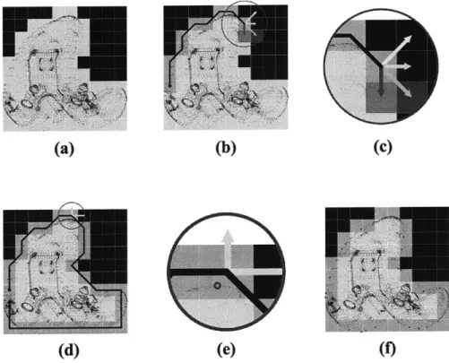
To decrease computation time and improve the robustness of the algorithm, only the outline points of the projected 3D model points are compared to the outlines of the TKA components. An outlining set of the projected points is determined by estab-lishing point connectivity and following an outer contour defined by the connectivity. Connectivity is determined by automatically compartmentalizing the model points so that a connected grid is produced (Fig. 3-2A). Using a left-looking, contour-following algorithm, the grids that outline the projected points are determined (Figs. 3-2B-C). For each contour grid, the point closest to the outside of the contour is selected (Figs.

3-2D-E). This automatic procedure results in a set of points that form an outline of

the projected 3D model points (Fig. 3-2F).

(a) (b) (c)

(d) (e) (f)

Figure 3-2: Outlining procedure. (A) Compartmentalize projected points (B-C) De-termine boundary grids with left-looking outlining technique (D-E) Select point in each grid that is closest to the outer edge. (F) Completion of algorithm with selected outline points.

3.1.4 Error Computation

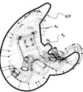
The minimum distance between each outlined, projected 3D model point and the fluoroscopic spline is determined (Fig. 3-3). Since the spline is represented as a parametric curve, the secant method is used to determine the minimum distance between a point and the spline (Eq. 3.4).

dki = mIn gk(t) - PkiI (3.4)

g'(

Ph,

.

Figure 3-3: Representation of calculating the minimum distance between projected points and a fluoroscopic outline.

model point, gk(t) is the parametric vector function of the fluoroscopic image spline, and t is the parametric variable, whose range corresponds to the recorded endpoints of the spline. For each intensifier, these distances are summed and divided by the total number of points, qk, resulting in a normalized distance. The normalized distances for each intensifier are then summed and returned as the value of the objective function, I (Eq. 3.5).

2 qk

I= qk E dki (3.5)

k=1 qk =1

3.2

Optimization

As the objective function, I, approaches zero the 3D model closely approaches the ac-tual TKA pose. Therefore, to accurately replicate the acac-tual TKA pose the objective function is minimized according to Eq. 3.6.

miT~) mn2 qk mn1

nyr) = Ey E y g (t) - Vk -(1;-Vk) (3.6)

The vector, r, holds the 6 optimization variables, r = (x, y, z, a, 3, 7), that

repre-sent the position and orientation of the models local coordinate system with respect to the global coordinate system. Any global optimization routine can be imple-mented to perform the minimization of the objective function, I(r), Eq. 3.5. Heuristic search methods, such as genetic algorithms and simulated annealing are also possible; however, simple quasi-Newton methods appear to have the fastest convergence with excellent results. Minimization of this function is accomplished with the Broyden, Fletcher, Goldfarb, and Shanno (BFGS) quasi-Newton method and implemented in Matlab software [5]. Utilizing the BFGS algorithm provides constrained line-search minimization of the performance index. The basic BFGS quasi-Newton method is formulated as a minimization of the quadratic in Eq. 3.7.

I(r) = -rTHr + cTr + b (3.7)

2

Where H is an approximation to the symmetric positive definite Hessian matrix of the objective function, c is a vector of constants defining constraints, while b is a scalar constant used to adjust for errors in approximating the Hessian. Minimization occurs by solving for the appropriate solution vector that solves Eq. 3.8.

VI(i) = Hi + c = 0 (3.8)

Solving Eq. 3.8 results in the solution vector i = -H-1c. The method of BFGS

then presents an iterative solution for the Hessian, H, presented in Eqs. 3.9-3.11.

GjIHT(sisj)Hj Hj+1 = Hj + 3 3 (3.9) Ts_%j 3 - sTH.sj 33 S3 = r,+1 - r3 (3.10) % = VI(rj+1) - VI(r,) (3.11)

can be calculated to determine the optimal solution. Global convergence is improved

by randomly perturbing the initial guess and submitting these additional guesses to

the optimization routine. Convergence for each run is controlled by terminating the minimization routine when the differential change in variables meets the required tol-erance or the quantity of objective function calls exceeds a specified number. Globally, runs that exceed the number of function calls and do not meet the required tolerance are deemed non-convergent. The remaining runs are used to determine a confidence interval and the match having the smallest performance index value is considered optimal.

3.3

Summary

Dual-orthogonal imaging can be applied to most of the articulating joints in the human body. This allows for highly accurate in-vivo study of joint kinematics and dynamics, cartilage contact and ligament interaction. The technique is especially attractive for in-vivo kinematics of patients with orthopaedic implants because 3D wire-frame models of the orthoses can be obtained directly from the CAD models used for manufacturing. Information gained from this imaging technique can be used for designing medical devices, clinical diagnosis and planning surgical procedures.

Automation of the procedure accelerates the matching process, stabilizes repeata-bility and reduces the learning curve required to produces accurate results. Automa-tion is accomplished by applying BFGS optimizaAutoma-tion to an iterative closest point objective function. Time savings from the algorithm allows for a large number of poses to be matched, making analysis of dynamic motion feasible. By formulating the matching problem as a mathematical process that can be computed, repeatability is gained and user bias is reduced. Automation also reduces the learning curve re-quired for determining an object's pose. Furthermore, statistical bounds of matching error are readily determined for the process. In short, automation of the matching process improves dual-orthogonal imaging by making it an easier and more robust tool to use, facilitating highly accurate biomechanics research.

Chapter 4

Validation and Application

Validation of the optimized matching algorithm was performed to demonstrate the accuracy and repeatability of recreating pose. The algorithms implemented in Matlab software were tested on a personal computer with a Pentium IV class processor (2.4 GHz, 512 MB RAM) running the Microsoft Windows XP Professional operating system. Validation consisted of running the algorithm with idealized, controlled, and real data using ten randomly generated initial pose estimates for each test. These tests were used to isolate various causes of error; idealized tests to isolate errors with geometry, standardized vitro tests to isolate errors caused by segmentation, and in-vivo tests to observe the combination of errors. For all tests the matching algorithm was set to record convergent solutions that did not exceed 800 objective function calls and had a differential tolerance of less than 0.0005 for each variable.

4.1

Idealized Environments

Idealized environments were created in order to determine the automated matching algorithms repeatability, accuracy, sensitivity to model point density and pose ori-entation, and optimal parameters under controlled conditions. These tests gave a basis for the ultimate potential of the algorithm. The idealized fluoroscopic setup was created by replicating the fluoroscopic environment using the 3D solid modeling software. Three-dimensional models were oriented in the virtual system in poses

ap-proximating a deep knee bend. From these poses the models were projected onto the virtual intensifiers, and the projections were used to create pseudo fluoroscopic out-lines. Models in this configuration were then considered to be the gold standard. The error of the matched poses was then determined by comparing the matched model poses to the gold standard.

4.1.1

TKA Components

Method

For the TKA components the 3D models of the femoral and tibial components were generated from manufacturer CAD data. With the idealized fluoroscopic setup the effect of model point density was tested for one pose of the tibial and femoral com-ponents (450 flexion position) using three different densities. The low point density models used a coarse mesh with approximately 3,500 points. Medium density point models were approximately 15,000 points and high density point models were made with over 20,000 points. Three additional poses (30, 60 and 900 flexion positions) for the medium point density models were matched to test the effect of pose orientation. For each pose ten estimates for the initial guess were created for each component by perturbing the models from the gold standard. The perturbations were created by randomly generating values for the pose variables within the range of ±20 mm and +20' using a Gaussian distribution. Next, the models were matched using fifty of the projected outline points. The accuracy and repeatability of the optimized matching algorithm in reproducing the femoral and tibial components position and orientation in 6DOF was recorded for each convergent match.

Results

Accuracy for the idealized tests was measured as the error between the body fixed local coordinate systems of the golden standard and the matched models. The sample standard deviation of these errors was selected as the measure of repeatability. Root-mean-square error (RMSE), or population standard deviation, values are also reported

for comparison with previous methods. Results for different densities of the femoral component are presented in Table 4.1. The pose of the femoral component was recreated to within 0.01+0.04 mm in translation and0.05t0.160 in rotation for the low point density model, 0.02+0.01 mm and 0.02±0.02 for the medium point density model, and 0.02±0.01 mm and 0.07±0.010 for the high point density model. The average time for matching a single pose was 200 see, 350 see, and 510 see for the low, medium, and high point density models, respectively. The average number of calls to the objective function was 640 for all model sizes. The results for four different flexion angles using the medium point density model are listed in Table 4.2. The average values of the pose variables were found to recreate pose to within 0.02+0.01 mm in translation and 0.02t0.03' in rotation.

3477 -0.001±0.016 [0.016] -0.006±0.037 [0.041] -0.009±0.021 [0.0301 0.007±0.030 [0.040] -0.050±0.099 [0.197] -0.038±0.160 [0.413] 14135 0.002±0.005 [0.014] -0.002±0.006 [0.0061 -0.018±0.012 [0.021] 0.004±0.004 [0.019] -0.017±0.020 [0.057] 0.015±0.019 [0.086] 21224 0.009±0.006 [0.024] -0.023±0.009 [0.0411 -0.005±0.003 [0.007] 0.002±0.008 [0.0111 0.068±0.006 [0.1021 -0.029±0.008 [0.047] 3608 -0.283±0.304 [0.403] 0.044±0.068 [0.078] 0.004±0.013 [0.013] 0.088±0.062 [0.106] -0.079±0.051 [0.0921 -0.747±0.706 [1.001] 14505 -0.069±0.043 [0.080] 0.029±0.018 [0.033] -0.009±0.003 [0.010] -0.163±0.080 [0.180] -0.042±0.036 [0.054] 0.069±0.102 [0.118] 35994 -0.049±0.018 [0.051] 0.016±0.009 [0.018] -0.011±0.003 [0.012] -0.074±0.010 [0.075] -0.011±0.010 [0.014] -0.189±0.104 [0.213]

Table 4.1: Accuracy (average error values), repeatability (standard deviations) and root-mean-square errors (RMSE) of the automatic matching procedure in an idealized environment using different model point densities. Accuracy and repeatability were evaluated for ten initial positions.

Results for the tibial component are presented in Table 4.1 for different densities of the model. Pose was recreated to within 0.28t0.30 mm in translation and 0.75+0.71' in rotation for the low density model, 0.07+0.04 mm and 0.16+0.100 for the medium point density model, and 0.05+0.02 mm and 0.19±0.10' for the high point density model. The average time for matching a single pose was 110 sec, 210 sec, and 220 see for the low, medium, and high point density models, respectively. For each model size

1 0.002±0.005 [0.0141 -0.002±0.006 [0.006] -0.018±0.012 [0.021] 0.004±0.004 [0.019] -0.017±0.020 [0.057] 0.015±0.019 [0.0861 2 -0.003±0.010 [0.010] -0.010±0.009 [0.013] -0.004±0.008 [0.008] 0.005±0.025 [0.023] 0.001±0.008 [0.007] -0.008±0.011 [0.012] 3 -0.000±0.009 [0.008] 0.001±0.014 [0.012] -0.001±0.005 [0.004] 0.005±0.011 [0.012] -0.003±0.021 [0.019] -0.009±0.023 [0.023] 4 -0.006±0.011 [0.011] -0.002±0.010 [0.009] 0.000±0.007 [0.006] -0.013±0.023 [0.025] 0.009±0.018 [0.018] -0.001±0.027 [0.024] 1 -0.069±0.043 [0.080] 0.029±0.018 [0.0331 -0.009±0.003 [0.010] -0.163±0.080 [0.1801 -0.042±0.036 [0.054] 0.069±0.102 [0.1181 -0.013±0.032 [0.033] 0.005O.024 [0.0241 -0.001±0.011 [0.010] 0.003±0.012 [0.0121 -0.005±0.019 [0.0191 -0.020±0.084 [0.083] 3 -0.010±0.057 [0.056] 0.010±0.170 [0.164] 0.013±0.034 (0.035] -0.009±0.023 [0.024] 0.011±0.043 [0.043] -0.042±0.138 [0.139] 4 0.012±0.096 [0.092] -0.008±0.041 [0.039] 0.003±0.025 [0.024] -0.004±0.051 [0.048] -0.013±0.041 [0.041] 0.163±0.389 [0.403]

Table 4.2: Accuracy (average error values), repeatability (standard deviations) and root-mean-square errors (RMSE) of the automatic matching procedure in an idealized environment using four different pose environments with a model point density of

15,000 points. Each position was evaluated for ten initial positions.

the average number of objective function calls was 650. Results from four different flexion angles for the medium point density model are listed in Table 4.2. The average values of the pose variables were found to recreate pose to within 0.07±0.09 mm in translation and 0.16±0.180 in rotation for the tibial component.

4.1.2

Natural Knee

Method

For the natural knee 3D models of the femur and tibia were generated from an MRI of a cadaver. Three poses (30, 60 and 90' flexion positions) for low point density models

(3,500 points) were matched to test the effect of pose orientation. For each pose ten

estimates for the initial guess were created for each model by perturbing them from the gold standard. The perturbations were created by randomly generating values for the pose variables within the range of ±20 mm and ±20' using a Gaussian distribution.

Next, the models were matched using fifty of the projected outline points. The accuracy and repeatability of the optimized matching algorithm in reproducing the

femoral and tibial components position and orientation in 6DOF was recorded for each convergent match.

Results

Accuracy for the idealized natural knee tests was measured as the error between the body fixed local coordinate systems of the golden standard and the matched models. The results for three different flexion angles using the medium point density model are listed in Table 4.3. The average error in recreating pose of the femur was 0.12±0.33 mm in translation and 0.14+0.31' in rotation. Average pose error for the tibia was 0.39±0.33 mm in translation and 0.23+0.20' in rotation. The sample standard deviation of these errors was selected as the measure of repeatability. The average time for matching a single pose was 30 seconds and the average number of calls to the objective function was 160.

1 0.00±0.36 [0.32] -0.01±0.34 [0.31] 0.04±0.11 [0.11] 0.05±0.06 [0.07] -0.01±0.03 [0.03] 0.04±0.19 [0.17]

2 0.08±0.07 [0.10] 0.38±0.32 [0.48] 0.06±0.33 [0.30] -0.15±0.25 [0.271 0.00±0.10 [0.09] -0.26±0.31 [0.38]

3 0.03±0.18 [0.17] 0.33±0.89 [0.86] 0.18±0.38 [0.38] -0.32±0.93 [0.89] 0.04±0.03 [0.05] -0.41±0.89 [0.89]

Error in Tibia Pose Parameters

1 -0.70±0.47 [0.81] -1.56±1.03 [1.811 -0.02±0.13 [0.11] -0.06±0.06 [0.08] 0.02±0.07 [0.07] 0.81±0.53 [0.941

2 0.01±0.11 [0.10] 0.07±0.19 [0.18] 0.03±0.09 [0.09] 0.05±0.08 [0.08] -0.01±0.05 [0.04] -0.02±0.11 [0.10]

3 0.09±0.11 [0.13] 0.59±0.46 [0.72] 0.42±0.39 [0.55] 0.46±0.37 [0.57] 0.09±0.14 [0.15] -0.53±0.43 [0.66]

Table 4.3: Accuracy (average error values), repeatability (standard deviations) and root-mean-square errors (RMSE) of the automatic matching procedure with an ideal-ized natural knee using three different pose environments with a model point density of 3,500 points. Each position was evaluated for ten initial positions.

4.2

Standardized In-vitro Environments

In an attempt to quantify accuracy of the system while in a working environment, controlled experiments were developed. The principle behind these tests was to image geometry with known structure and position. This was accomplished by employing

highly precise geometry to enforce a relative distance and also by accurately

trans-lating known geometry.

4.2.1

Spheres

Method

A standardized test in the manner of Short, et al was performed consisting of eight

spheres 12.70 mm in diameter each having a tolerance of +0.01 mm[24]. Five of the spheres were stainless steel, two were ceramic (spheres 2 & 7), and one was tungsten (sphere 5). The spheres were arranged in a fixed pattern (Fig. 4-2) and imaged with the dual-orthogonal fluoroscopic system.

Figure 4-1: A virtual environment for the standardized in-vitro sphere test.

Using the solid modeling program a spherical model 12.70 mm in diameter was created and converted into a point cloud containing 2,500 points. Next, the model was placed centrally in the virtual fluoroscopic environment. Then, ten estimates for the initial pose were created for each component by perturbing the model from the placed configuration. The perturbations were created by randomly generating values for the pose variables within the range of t20 mm using a Gaussian distribution. Next, the

Figure 4-2: Geometry of standardized test. Spheres two and seven were ceramic, sphere five was tungsten and the remaining spheres were stainless steel. The spheres were stacked in the vertical plane.

models were matched using sixty of the projected outline points and the convergent matches were recorded. The accuracy of the matching algorithm was determined by comparing the distance between the adjacent matched spheres and the true distance of one diameter, 12.70 mm. 1 to 2 12.76 ± 0.04 [0.07] 2 to 3 12.72 ± 0.03 [0.03] 3 to 4 12.56 ± 0.01 [0.14] 4 to 5 12.72 ± 0.02 [0.03] 5 to 6 12.66 ± 0.04 [0.06] 6 to 7 12.75 ± 0.06 [0.07] 7 to 8 12.68 ± 0.05 [0.06]

Table 4.4: Standardized test validating accuracy and precision of the dual-orthogonal fluoroscopic system under actual conditions with spheres of different materials using ten initial positions.

Results

For the standardized test, the distance between each adjacent pair of spheres was calculated (Table 4.4). A maximum distance of 12.76 mm was calculated between sphere 1 and sphere 2 and a minimum distance of 12.56 mm was calculated between

sphere 5 and sphere 6. The average distance between matched pairs of adjacent spheres was 12.69 mm, 0.01 mm less than the actual distance data, with a standard deviation of +0.06 mm. The average time for each match of a single sphere was 15

sec with 380 calls to the objective function.

4.2.2

Natural Knee

Method

For the natural knee 3D medium point density models (15,000 points) of the femur and tibia were generated from an MRI of a cadaver. The cadaver knee was mounted in a tensile testing machine (QTest 5, MTS, Minneapolis, MN), which has a linear accuracy of 0.001 mm. The knee was then imaged as it was translated to five positions: 0, 2, 5, 10, 15 mm. The translation distance between poses was considered the gold standard. For each pose ten estimates for the initial guess were created for each model

by perturbing them an initial match. The perturbations were created by randomly

generating values for the pose variables within the range of +20 mm and ±200 using a Gaussian distribution. Next, the models were matched using fifty of the projected outline points. The accuracy and repeatability of the optimized matching algorithm in reproducing the femoral and tibial position and orientation in 6DOF was recorded for each convergent match.

Results

Accuracy for the standardized natural knee tests was measured as the error between the translation of three body fixed points and the known displacement imposed by the tensile testing machine. The distance from the initial position was calculated for each position and listed in Table 4.5. The average error was found to be 0.14 mm for the femur and 0.54 mm for the tibia. Repeatability of all poses was found to be less than +0.85 mm, where the sample standard deviation of these errors was selected as the measure of repeatability. The average time for matching a single pose was 90 seconds and the average number of calls to the objective function was 500.

5 0.20 ± 1.25 0.47 ± 0.95

10 -0.05 ± 0.69 0.31 ± 0.82

15 -0.02 ± 0.58 0.82 ± 0.91

Table 4.5: Standardized test validating accuracy and precision of the dual-orthogonal fluoroscopic system under actual conditions with a cadaver knee translated known distances.

4.3

In-vivo Environments

Testing the algorithm with actual subjects is the most important validation of perfor-mance. In-vivo validation utilizes images acquired from living subjects and provides a metric for determining the algorithm's repeatability. TKA subjects were imaged performing a lunge activity and this data was used for the validation.

4.3.1

TKA Components

Method

In-vivo images taken with the dual fluoroscopic system of the right knee of a patient after TKA. The images were acquired under IRB approval and with informed consent of the patient. The patient had a cruciate retaining component and images were taken during a lunge (NexGen CR TKA, Zimmer, Inc, Warsaw). Poses selected for matching were for images taken at 100 and 50' of flexion of the patient. Using the solid modeling program the component models were converted into point clouds containing

15,000 points. Next, the models were manually matched to the fluoroscopic contours

in the virtual fluoroscopic environment. Then, for both flexion angles each model

lowpir