Exponentially decaying boundary layers as limiting cases of families of algebraically decaying ones

0044-2275/06/050777-16 c

° 2006 Birkh¨auser Verlag, Basel Mathematik und Physik ZAMPZeitschrift f¨ur angewandte

Exponentially decaying boundary layers as limiting cases of

families of algebraically decaying ones

Shijun Liao and Eugen Magyari

Abstract. The boundary value problem for the similar stream function f = f (η; λ) of the

Cheng–Minkowycz free convection flow over a vertical plate with a power law temperature dis-tribution_Tw(_{x) = T∞}+_Axλin a porous medium is revisited. It is shown that in the_λ-range

−1/2 < λ < 0 , the well known exponentially decaying “first branch” solutions for the velocity

and temperature fields are not some isolated solutions as one has believed until now, but limiting cases of families of algebraically decaying multiple solutions. For these multiple solutions well converging analytical series expressions are given. This result yields a bridging to the historical quarreling concerning the feasibility of exponentially and algebraically decaying boundary lay-ers. Owing to a mathematical analogy, our results also hold for the similar boundary layer flows induced by continuous surfaces stretched in viscous fluids with power-law velocitiesuw(x) ∼ xλ.

Mathematics Subject Classification (2000). 76D10, 76S05, 76M99.

Keywords. Boundary layers, similarity, porous media, algebraic decay, homotopy analysis.

1. Introduction and summary of the previous results

f000+λ + 1 2 f f

00_{− λf}02_{= 0}

f (0; λ) = 0, f0(0, λ) = 1, f0(∞; λ) = 0

(1) for the similar stream function f = f (η; λ) of the free convection boundary layer flow over a vertical plate immersed in a porous medium as being first formulated by Cheng and Minkowycz, [1]. The plate is assumed impermeable and its temperature distribution is of the power-law form, T_w(x) = T_∞+Axλ. The velocity components and the temperature field are given in terms of f (η) as follows

u = [ρ_∞gβK(T_w− T_∞)/µ]f0(η; λ) v = 1 2[αρ∞gβK(Tw− T∞)/µx] 1/2_{[(1− λ)ηf}0_{− (1 + λ)f]} T = T_∞+ (T_w− T_∞)f0(η; λ) (2) DOI 10.1007/s00033-006-0061-x

(everywhere the original notation of Cheng and Minkowycz is used).

Cheng and Minkowycz, [1], solved the problem (1) numerically in the range 1/3 < λ < 1. A comprehensive study has then performed by Ingham and Brown, [2]. Later, several analytical and numerical solutions of this problem were collected and discussed in the monograph of Pop and Ingham [3]. The main results reported by Ingham and Brown, [2] may be summarized as follows.

1. The Cheng–Minkowycz problem (1) does admit solutions only in the parameter range λ >−1/2.

2. In the range−1/2 < λ < 0 both f and f0 are non-negative for all η≥ 0. 3. For λ = +1 and λ = −1/3 elementary analytical solutions exist (see also

below).

4. For λ > 1 a second branch of solutions exists.

5. For the dimensionless wall temperature gradient f00(0; λ) the integral relation-ship f00(0; λ) =−3λ + 1 2 ∞ Z 0 f02(η; λ)dη (3)

holds. However, it is important to underline here that this relationship is valid only for the solutions which satisfy the asymptotic condition

lim

η→∞f (η; λ)f

0_{(η; λ) = 0. (4)}

Obviously, the exponentially decaying solutions f ≡ f_exp(η; λ) satisfy this con-dition. Thus, for these solutions Eq. (3) implies

f_exp00 (0; λ) = 0 for λ =−1 3 (5a) and sgn£f_exp00 (0; λ)¤=−sgn µ λ +1 3 ¶ for λ6= −1 3. (5b)

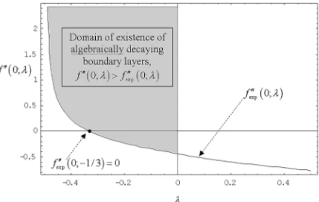
The dependence of f_exp00 (0, λ) on λ, as calculated by Ingham and Brown [2] is shown in Fig. 1. The domain of existence of the algebraically decaying solutions, the main issue of the present paper, is also shown in Fig. 1. The details will be discussed in Sections 2 and 3 below.

6. Ingham and Brown [2] also gave valuable estimates of f_exp00 (0; λ) for 0 < λ + 0.5 << 1 as well as for λ near to zero. These are:

f_exp00 (0; λ) = 0.078103· (λ + 0.5)−3/4 (6) for 0 < λ + 0.5 << 1, and

f_exp00 (0; λ) =−0.44375 − 0.85665 · λ + 0.66943λ2 (7) for|λ| << 1, respectively.

Figure 1. In the range−1/2 < λ < 0, the whole domain f00(0;λ) > f_exp00 (0;λ) above the Ingham–Brown characteristic curvef_exp00 (0;λ) corresponding to the exponentially decaying solutions is densely “filled” with values off00(0;λ) corresponding to algebraically decaying solutions.

A comprehensive analytical and numerical investigation (for a slightly rescaled form) of the boundary value problem (1) as it occurs in the context of the boundary layer flows induced by continuous surfaces stretched with power-law velocities has been reported by Banks, [4].

Recently for the exponentially decaying solutions f≡ f_exp(η; λ) of the problem (1) analytical expressions in form of infinite series with controllable convergence have been given by Liao and Pop, [5] by applying the homotopy analysis method (Liao, [6]). This method allows for the calculation of the similar wall temperature gradient f_exp00 (0; λ) and of the similar entrainment velocity f_exp(∞; λ) to any desired precision.

2. Algebraically decaying solutions

2.1. General features

We first examine the general question of the existence in the parameter range

−1/2 < λ < 0 of similar velocity and temperature profiles f0_{(η; λ) with algebraic}

asymptotic decay of the form

f0(η; λ)∼ ηb as η→ ∞ (8a)

which yields

f (η; λ)∼ 1 b + 1η

b+1 _{as η→ ∞ (8b)}

where b is a constant. As a requirement of the boundary condition f0(∞; λ) = 0, the exponent b must be negative. Substituting (8) in Eq. (1) and balancing the

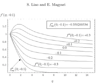
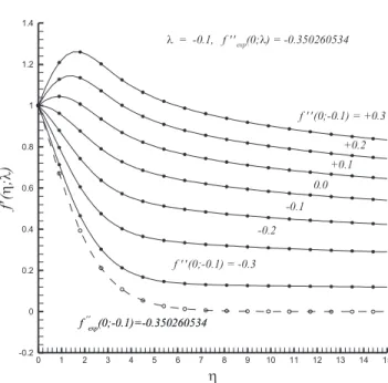
Figure 2. Here the exponentially decaying and seven (presumably) algebraically decaying dimensionless temperature (and velocity) profilesf_exp0 (η; λ) and f0(η; λ) are shown for

λ = −0.1. The exponentially decaying profile corresponds to the value f00

exp(0;−0.1) = −0.350260534 of the dimensionless wall temperature gradient. As f00(0;−0.1) approaches the value off_exp00 (0;−0.1), the family of algebraically decaying profiles goes over continuously in the exponentially decaying one.

dominant terms, we obtain that in the range−1/2 < λ < 0 which we are interested in, the asymptotic behavior (8) is possible for b = 2λ/(1−λ) which further implies

b + 1≡ β = 1 + λ

1− λ with 0 < β < 1. (9) Substituting Eqs. (8) in Eq. (4) we easily deduce that this condition is satisfied by the algebraically decaying solutions only in the range−1/2 < λ < −1/3 and it is violated in the remaining part −1/3 ≤ λ < 0 of the interval of interest

−1/2 < λ < 0. Hence, Eq. (5b) which is a consequence of Eq. (3), holds also

for our algebraically decaying solutions, but only in the range−1/2 < λ < −1/3 where f00(0; λ) > f_exp00 (0; λ) > 0. For−1/3 ≤ λ < 0 where f_exp00 (0; λ) ≤ 0, in the existence domain f00(0; λ) > f_exp00 (0; λ) of the algebraically decaying solutions both negative and positive values of f00(0; λ) are possible.

The numerical “proof” for the existence domain f00(0; λ) > f_exp00 (0; λ) of the multiple solutions for−1/2 < λ < 0 is straightforward. It is illustrated in Fig. 2 where the exponentially decaying and a couple of (presumably) algebraically de-caying dimensionless temperature (and velocity) profiles f_exp0 (η; λ) and f0(η; λ), respectively, are shown for λ =−0.1. All these profiles have been obtained by a direct numerical solution of the problem (1). The exponentially decaying solution corresponds to the value f_exp00 (0;−0.1) = −0.350260534 of the dimensionless wall temperature gradient. All the values f00(0;−0.1) > f_exp00 (0;−0.1) = −0.350260534 furnish (presumably) algebraically decaying solutions of the problem (1).

We underline again that the plots of Fig. 2 only show that the asymptotic decay of the solutions corresponding to values f00(0;−0.1) > f_exp00 (0;−0.1) is slower

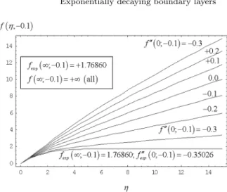
Figure 3. Plots of the stream functionsf(η; λ) corresponding to the velocity profiles of Fig. 2. All the curves corresponding tof00(0;−0.1) > f_exp00 (0;−0.1) go to infinity as η → ∞, while that corresponding tof_exp00 (0;−0.1) = −0.35026 goes to the finite asymptotic value

fexp(∞; −0.1) = +1.76860.

than the decay of the profile associated with the value f_exp00 (0;−0.1) lying on the Ingham–Brown curve of Fig. 1, i.e. it only suggests but it does not rigorously prove the algebraic character of their asymptotic behavior. Nevertheless, this conjecture is substantiated once more by Fig. 3 where the plots of the stream functions f (η; λ) corresponding to the velocity profiles of Fig. 2 are shown. We see in Fig. 3, that all the curves corresponding to f00(0;−0.1) > f_exp00 (0;−0.1) go to infinity as η → ∞, while that corresponding to f_exp00 (0;−0.1) is the only one which goes to a finite asymptotic value, f_exp(∞; −0.1) = +1.76860527.

2.2. The caseλ = −1/3

As it has been shown recently by Magyari et al. [7], the algebraically decaying solutions of the boundary value problem (1) corresponding to the values f00(0; λ) >

f_exp00 (0; λ) of f00(0; λ) can be obtained for λ = −1/3 in an exact analytic form in terms of the Airy functions,

f (η;−1/3) =£36f00(0;−1/3)¤1/3Bi

0_(z

0)Ai0(z)− Ai0(z0)Bi0(z)

Bi0(z₀)Ai(z)− Ai0(z₀)Bi(z) (10a)

f0(η;−1/3) = f00(0;−1/3) · η + 1 −1 6f

2 _(10b)

where

The far field behavior of this solution is

f (η;−1/3) →p6 + 6f00(0;−1/3)η as η → ∞ (12a)

f0(η;−1/3) → 3f00(0;−1/3)¡6 + 6f00(0;−1/3)η¢−1/2 as η→ ∞ (12b) for all f00(0;−1/3) > f_exp00 (0;−1/3) = 0. Hence, in this special case the values of the exponents present in Eqs. (8) are b =−1/2 and β = +1/2. Now, we actually see that, as already mentioned above, the condition (4) of validity of the integral relationship (3) is not satisfied in this case.

A remarkable feature of the solution (10a) having for f00(0) > 0 the algebraic asymptotic behavior (12a) is that for f00(0) → 0 it goes over in the well known hyperbolic tangent solution f (η;−1/3) = √6 tanh¡η/√6¢. This property has been proved by Magyari et al. [7] numerically, and later by Magyari and Rees [8] analytically. The analytical proof uses the asymptotic properties of the Airy functions (see e.g. [9]) and yields

f (η;−1/3) →¡6 + 6f00(0;−1/3)η¢−1/2· tanh µ¡ 1 + f00(0;−1/3)η¢3/2− 1 (27/2)1/2f00(0;−1/3) ¶ → √ 6 tanh µ η √ 6 ¶ (13) as f00(0;−1/3) → 0. In this way for f00(0;−1/3) = 0 one obtains f0(η;−1/3) = 1/ cosh2¡η/√6¢ which shows explicitly that the family of solutions f0(η;−1/3) having for f00(0;−1/3) > 0 the algebraic asymptotic decay (12b) goes over for

f00(0;−1/3) → 0 in a solution which decays exponentially, f0(η;−1/3) → 4 exp¡− 2η/√6¢. as η → ∞. The main issue of the present paper is to prove this remarkable feature, i.e. the continuous crossover of a family of algebraically decaying boundary layers into an exponentially decaying one, holds for the whole parameter range−1/2 < λ < 0 of the boundary value problem (1). The numerical “proof” has already been illustrated in Fig. 2. The detailed analytical proof is presented in the Appendix and its main results are summarized in Sect. 2.3 below.

2.3. Series solutions

With the aid of the homotopy analysis method (Liao, [6]) we obtain the following series solution of the problem (1):

f (η; λ) = 1 α +∞ X k=0 2k+2_X n=1 2k+1+[n/2]_X m=n−1+Xn An,m_k (1 + αη)nβ−m. (14)

Here [x] stands for the integer part of a real number x, α > 0, is a constant, and the coefficients Am,n_k can recursively be calculated from the equations

An,m_k = ~ ¡ α2B_kn,m+ C_kn,m¢ (nβ− m − β)(nβ − m − β + 1)(nβ − m − 2β + 2) + An,m_k−1X_2k+2−nX_{2k+1+[n/2]−m} (15) where~ is an auxiliary parameter, nβ − m 6= β, β − 1, 2β, β − 2 and

B_kn,m=X_2k+2−nX_{2k+3−m+[n/2]}X_m+1−n−Xn(nβ−m+ 2)(nβ−m+1)(nβ−m)An,m−2_k−1 , (16) C_km,s= k−1 X n=0 min{2n+2,m−1}_X p=max{1,m+2n−2k} min{2n+1+[p/2],s+p−m−X_X m−p} q=max{p−1+Xp,s+2n−2k−[(m−p)/2]} XmX2k−s+3+[p/2]+[(m−p)/2]Xs+3−m−Xp−Xm−p ×[(m−p)β+q−s+1] ½ (1 + λ) 2 [(m−p)β+q−s]−λ(pβ−q) ¾ Ap,q_n Am−p,s−q−1_k−1−n (17) and A1,0_k =2(β− 1) 2_δ 0+ (4− 3β)δ1+ δ2 β− 2 , A1,1_k =−2βδ₀+ 3δ₁− δ2 (β− 1), A2,2_k =β(1− β)δ0− 2(1 − β)δ1− δ2 (β− 1)(β − 2) . (18)

In the latter equations,

δ₀= 2k+2_X n=1 2k+1+[n/2]_X m=n−1+Xn An,m_k X_(n−1)2_+m2₊₁X_(n−1)2_+(m−1)2₊₁X_(n−2)2_+(m−2)2₊₁, δ1= 2k+2_X n=1 2k+1+[n/2]_X m=n−1+Xn An,m_k (nβ−m)X_(n−1)2_+m2₊₁X_(n−1)2_+(m−1)2₊₁X_(n−2)2_+(m−2)2₊₁, δ₂= 2k+2_X n=1 2k+1+[n/2]_X m=n−1+Xn An,m_k (nβ− m)(nβ − m − 1)× X(n−1)2_+m2₊₁X_(n−1)2_+(m−1)2₊₁X_(n−2)2_+(m−2)2₊₁. (19) In above expressions, γ = f00(0; λ) (20)

is given (see the existence domain shown in Fig. 1) andX_k is defined by

Xk =

(

0, k≤ 1,

The first three coefficients are A1,0₀ = 4− 3β + γα −1 2− β , A 1,1 0 = 3− 3β + γα−1 β− 1 , A 2,2 0 = 2− 2β + γα−1 (1− β)(2 − β). (22) Further details are presented in the Appendix of the present paper.

In terms of the first three coefficients (22) we can obtain all coefficients of the expansion (14) one by one, both symbolically or numerically. In this way the series solution (14) with algebraic asymptotic decay is fully determined. For example, for the parameter values λ =−1/3, γ = 1, α = 1/2 and ~ = −4 we obtain:

A1,0₀ = 3, A1,1₀ =−7, A2,2₀ = 4, A1,0₁ =−3079 2520, A 1,1 1 = 1331₇₂ , A1,21 = 9₈, A1,31 =35₂₄, A2,2₁ =−36, A2,3₁ = 784 45 , A 2,4 1 =−48₃₅, A3,3₁ = 12, A3,4₁ =−140 9 , A4,4₁ = 0, A4,5₁ = 128 35 , (23) . . . . and thus f µ η;−1 3 ¶ =4481 1260 µ 1+1 2η ¶1 2 +827 36 µ 1+1 2η ¶−1 2 −64 µ 1+1 2η ¶−1 +105 4 µ 1+1 2η ¶−3 2 +1568 45 µ 1+1 2η ¶−2 −1015 36 µ 1+1 2η ¶−5 2 +32 7 µ 1+1 2η ¶−3 +. . . (24)

3. Discussion and conclusions

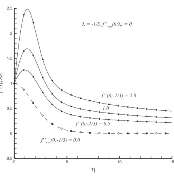
As shown in Fig. 4, for λ =−1/3 the series solution (14) agrees well with the exact solution (10) already in the 20th-order of approximation, and its convergence can further be accelerated by means of the homotopy–P´ade technique (Liao, [6]). This verifies the validity of the homotopy approach applied.

The expression (24) of f (η;−1/3) obtained by truncation of (14) yields an accurate approximation for small values of η. It also describes the asymptotic behaviour of f (η;−1/3) with an acceptable accuracy. Indeed, for η → ∞ the leading order term of (24) behaves as

f µ η;−1 3 ¶ =√2(A1,0₀ + A1,0₁ )√η =√2 µ 3−3079 2520 ¶ √ η = 2.514718·√η. (25) This fits the asymptotic expression (12a) of the exact solution (10a),

f_exact µ η;−1 3 ¶ =p6f00(0;−1/3)η =√6·√η = 2.449489·√η (26)

Figure 4. Comparison of the algebraically decaying series solutions (14) (filled circles)

associated with different positive values off00(0;−1/3), with the analytic solution (10) valid for

λ = −1/3 (lines). The dashed line correspond to the well known exponentially decaying

solutionf_exp0 (η; −1/3) = 1/ cosh2(η/√6) withf00(0;−1/3) = 0. The open circles on this curve denote series solution given by Liao and Pop, [5]. Asf00(0;−1/3) approaches the value

f00

exp(0;−1/3) = 0, the family of algebraically decaying profiles goes over continuously in the

exponentially decaying one.

with a deviation of only +2.7%.

The accuracy of the leading order term of (24) can obviously be enhanced by taking into account in (14) several terms the degree (1 + η/2)1/2. By doing so, one obtains f µ η;−1 3 ¶ =µ√2· m X n=0 A1;0_n ¶ √ η as η→ ∞. (27)

One finds that for m = 40 in (27) the coefficient of√η in (27) approaches (although

not monotonously) the value 2.4496.

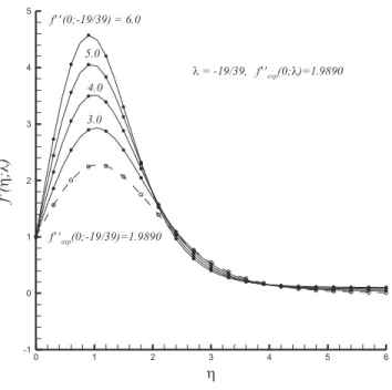
In general, for any specified λ∈ (−1/2, 0) we can get convergent algebraically decaying series solution for any f00(0; λ) > f_exp00 (0; λ) in a similar way by choosing the values of the control parameters α and~ suitably. On the other hand, we fail to get any convergent series solutions if f00(0; λ) < f_exp00 (0; λ), in a full agreement with the existence domain shown in Fig. 1. As an illustration, in Figs. 5 and 6 the

Figure 5. Comparison of the series solution (symbols) with the numerical results (lines) for

λ = −1/10. The dashed and solid lines correspond to the exponentially decaying and the seven

algebraically decaying dimensionless temperature (or velocity) profilesf_exp0 (η; λ) and f0(η; λ), respectively. The open circles denote exponentially decaying series solution given by Liao and Pop, [5], and the filled circles are the algebraically decaying series solution obtained in this article. Asf0(η; λ) approaches the value of f_exp0 (η; λ), the family of algebraically decaying profiles goes over continuously in the exponentially decaying one.

cases λ =−1/10 and λ = −19/39 ≈ −0.4872 are presented, respectively.

Therefore, the solutions obtained by the homotopy analysis method and pre-sented in Sect. 2.3 (with details in the Appendix) prove the main result of the present paper that in the parameter range −1/2 < λ < 0 of the Cheng and Minkowycz problem (1) the well known exponentially decaying solutions are not some isolated solutions but limiting cases of families of algebraically decaying multiple solutions. In other words, in the range−1/2 < λ < 0 the points of the Ingham–Brown curve f_exp00 (0; λ) shown in Fig. 1 are in fact branching points. From every point of this curve there bifurcates a whole family of algebraically decaying solutions corresponding to values f00(0; λ) > f_exp00 (0; λ) of the dimensionless wall temperature gradient. In addition to the different asymptotic decay of the dimen-sionless temperature (and velocity) fields f0(η; λ) associated with the points of the Ingham–Brown curve f_exp00 (0; λ) on the one hand and with the values of f00(0; λ) above it, f00(0; λ) > f_exp00 (0; λ), the corresponding entrainment velocities f (∞; λ)

are also basically different, as already predicted numerically (see Fig. 2). Indeed, while fexp(∞; λ) is a finite quantity, in the case of the bifurcating algebraically decaying solutions f (η; λ)→ ∞ as η → ∞. These diverging entrainment velocities are given according to Eq. (14) by

f (η, λ) = αβ−1 Ã _m X n=0 A1,0_n ! · ηβ _{as η→ ∞. (28)}

Appendix: Derivation of the series solution (14)

Consider the solutions with algebraic asymptotic property at infinity

f ∼ aηβ, η→ +∞, (A-1)

where β is defined by Eq. (9). When−1/2 < λ < 0, it holds 2β− 2 < β − 1 < β < 1. Under the transformation

f (η; λ) = g(ξ; λ)/α, ξ = 1 + αη, α > 0,

the original equation becomes

α2gm(ξ; λ) + µ 1 + λ 2 ¶ g(ξ; λ)g00(ξ; λ)− λ[g0(ξ; λ)]2= 0 (A-2) subject to the boundary conditions

g(1; λ) = 0, g0(1; λ) = 1, g0(+∞; λ) = 0, (A-3) where the primes denote the differentiation with respect to ξ.

According to the algebraic property at infinity, (A-1), and the boundary con-ditions (A-3), the solution can be expressed by the following set of base functions

© ξmβ−n|mβ − n < 1, β < 1, m ∈ N, n ∈ Nª in the form g(ξ; λ) = b_1,0ξβ+ +∞ X m=1 +∞ X n=1 b_m,nξm(β−n), (A-4) which provides us with the so-called Rule of Solution Expression suggested by Liao, [6]. Note that a solution expressed by the Rule of Solution Expression (A-4) automatically satisfies the boundary condition at infinity, i.e. g0(+∞; λ) = 0, which therefore becomes a non-effective boundary condition. The problem can be closed by providing an additional boundary condition f00(0; λ) = γ, corresponding to

g00(1; λ) = γ/α, (A-5)

Figure 6. Comparison of the series solution (symbols) with the numerical results (lines) for

λ = −19/39. The dashed and solid lines correspond to the exponentially decaying and the four

algebraically decaying dimensionless temperature (or velocity) profilesf_exp0 (η; λ) and f0(η; λ), respectively. The open circles denote exponentially decaying series solution given by Liao and Pop, [5], and the filled circles are the algebraically decaying series solution obtained in this article. Asf0(η; λ) approaches the value of f_exp0 (η; λ), the family of algebraically decaying profiles goes over continuously in the exponentially decaying one.

According to the Rule of Solution Expression (A-4) and the boundary condi-tions (A-3) and (A-5), it is straightforward to choose an initial approximation

g₀(ξ; λ) = (4− 3β + γα−1) (2− β) ξ β₋(3− 3β + γα−1) (1− β) ξ β−1 +(2− 2β + γα −1₎ (1− β)(2 − β) ξ 2β−2_. (A-6)

From Eq. (A-2) and the Rule of Solution Expression (A-4), we choose the auxiliary linear operator

L[f] = ξ3_f000

+ a₂(ξ)ξ2f00+ a₁(ξ)ξf0+ a₀(ξ)f, (A-7) where the primes denote the differentiation with respect to ξ, a₀(ξ), a₁(ξ), a₂(ξ) are

unknown functions to be determined soon. Enforcing the first three base functions

ξβ, ξβ−1, ξ2β−2

to be the solutions of the linear equationL[f] = 0, we have

a₀=−2β(1 − β)2, a₁= (β− 1)(5β − 6), a₂=−2(2β − 3).

Thus, to obey the Rule of Solution Expression (A-4), it is natural for us to choose the linear auxiliary operator

L[f] = ξ3_f000_{− 2(2β − 3)ξ}2_f00_{+ (β− 1)(5β − 6)ξf}0_{− 2β(β − 1)}2_{f, (A-8)} which possesses the property

L£C0ξβ+ C1ξβ−1+ C2ξ2β−2¤= 0, (A-9) for any constants C0, C1 and C2. Besides, we are led from Eq. (A-2) to define a nonlinear operator N[φ(ξ; λ, q)] = α2∂3φ(ξ; λ, q) ∂ξ3 + µ 1 + λ 2 ¶ φ(ξ; λ, q)∂ 2_{Φ(ξ; λ, q)} ∂ξ2 − λ · ∂φ(ξ; λ, q) ∂ξ ¸₂ , (A-10)

where q ∈ [0, 1] is an embedding parameter. Let ~ denote a non-zero auxiliary parameter, H(ξ) a non-zero auxiliary function, and q ∈ [0, 1] is an embedding parameter. We construct the so-called zeroth-order deformation equation

(1− q)L[φ(ξ; λ, q) − g₀(ξ; λ)] = q~H(ξ)N[φ(ξ; λ, q)], (A-11) subject to the boundary conditions

φ(1; λ, q) = 0, ∂φ(ξ; λ, q) ∂ξ ¯¯ ¯¯ ξ=1 = 1, ∂ 2_{φ(ξ; λ, q)} ∂ξ2 ¯¯ ¯¯ ξ=1 = γ α, ∂φ(ξ; λ, q) ∂ξ ¯¯ ¯¯ ξ→+∞ = 0. (A-12)

Obviously, when q = 0, we have from Eqs. (A-11) and (A-12) the solution

φ(ξ; λ, 0) = g₀(ξ; λ). (A-13) When q = 1, Eqs. (A-11) and (A-12) are equivalent to the original ones (A-2), (A-3) and (A-5), provided

φ(ξ; λ, 1) = g(ξ; λ). (A-14) Thus, as q increases from 0 to 1, the solution φ(ξ; λ, q) of the zeroth-order defor-mation equations (A-11) and (A-12) varies from the initial approxidefor-mation g₀(ξ; λ) to the solution of the original equations (A-2), (A-3) and (A-5).

Assume that~ and H(ξ) are properly chosen so that the variation (or deforma-tion) is smooth enough and thus φ(ξ; λ, q) can be expanded in the Taylor series

φ(ξ; λ, q) = φ(ξ; λ, 0) + +∞ X k=1 g_k(ξ; λ)qk, (A-15) where g_k(ξ; λ) = 1 k! ∂ + kφ(ξ; λ, q) ∂qk ¯¯ ¯¯ q=0 ,

and besides the series (A-15) converges at q = 1. Then, using (A-13) and (A-14), we have the solution series

g(ξ; λ) = g₀(ξ; λ) + +∞ X

k=1

g_k(ξ; λ). (A-16)

which provides us with a relationship between the solution g(ξ; λ) and the initial guess g0(ξ; λ).

Define the vector

− →_g

k=©g0(ξ; λ), g1(ξ; λ), g2(ξ; λ), . . . , gk(ξ, λ)ª.

To obtain governing equation and boundary conditions for the unknown g_k(ξ; λ) in the order k = 1, 2, 3, . . ., we differentiate the zeroth-order deformations (A-11) and (A-12) k times with respect to the embedding parameter q, then divide them by

k!, and finally set q = 0. In this way, we have the so-called k th-order deformation

equation

L[gk(ξ; λ)− Xkgk−1(ξ; λ)] =~H(ξ)Rk(−→gk−1), (A-17)

subject to the boundary conditions

g_k(1; λ) = g0_k(1; λ) = g00_k(1; λ) = g_k0(+∞; λ) = 0, (A-18) where R_k(−→g_k−1) = α2(g_k−1)000+ k−1 X n=0 "Ã 1 + λ 2 ! g_n(g_k−1−n)00−λ(g_n)0(g_k−1−n)0 # (A-19) and Xk = ( 0, k≤ 1, 1, k > 1. (A-20)

Note that, substituting (A-15) in Eqs. (A-11) and (A-12), and equating the co-efficients of the same powers of q, we can obtain the same equations as given above.

To obey the Rule of Solution Expression (A-4), the auxiliary function H(ξ) must be in the form H(ξ) = ξµ, where µ is an integer to be determined. It is found that, when µ ≥ 2, R_k(−→g_k−1) contains the term ξ2β−2, and thus, due to (A-9), the solution g_k(ξ) has the term ξ1nξ. However, the term ξ1nξ disobeys the

Rule of Solution Expression (A-4). When µ≤ 0, the solutions of the high-order deformation equations do not contain the term ξ2β−1. This, however, disobeys the Rule of Coefficient Ergodicity, i.e. coefficients of all base functions could be modified as the order of approximation tends to infinity, as suggested by Liao (2003). Thus, we must choose µ = 1, corresponding toH(ξ) = ξ. In this way, all of the linear equations (A-18) and (A-19) have solutions which comply the Rule of Solution Expression (A-4). And it is found that g_k(ξ; λ) can be expressed in such a general form g_k(ξ, λ) = 2k+2_X n=1 2k+1+[n/2]_X m=n−1+Xn An,m_k ξnβ−m, k = 0, 1, 2, 3,· · · (A-21)

where An,m_s is a constant coefficient, the operator [x] takes the integer part of the number x. Substituting (A-21) into (A-19), we have

R_k= 2k+2_X n=1 2k+1+[n/2]_X m=n−1+Xn ¡ α2B_kn,m+ C_kn,m¢ξnβ−m−1, where B_kn,m=X_2k+2−nX_{2k+3−m+[n/2]}X_m+1−n−Xn(nβ−m+2)(nβ−m+1)(nβ−m)An,m−2_k−1 , and C_km,s= k−1 X n=0 min{2n+2,m−1}_X p=max{1,m+2n−2k} min{2n+1+[p/2],s+p−m−XX m−p} q=max{p−1+Xp,s+2n−2k−[(m−p)/2]} XmX2k−s+3+[p/2]+[(m−p)/2]Xs+3−m−Xp−Xm−p × [(m − p)β + q − s + 1] ½ 1 + λ 2 [(m− p)β + q − s] − λ(pβ − q) ¾ Ap,q_n Am−p,s−q−1_k−1−n .

Substituting these expressions into the high-order deformation equations (A-18) and (A-19), we obtain the recurrence formulas given in section 3.2. The first three coefficients A1,0₀ , A1,1₀ , A2,2₀ are obtained by comparing (A-21) with the initial guess (A-6).

The above recurrence formulas contain two auxiliary parameters, α > 0 and ~. The value of α > 0 is determined by the minimum value of the residual error of the governing equation about the initial guess (A-6). Then, only the auxiliary parameter~ is unknown, which provides us with a simple way to control and adjust the convergence of the series (A-16), as shown by Liao, [5]. In all cases considered in this articles, we choose α = 1/2 and~ = −4.

References

[1] P. Cheng and W. J. Minkowycz, Free convection about a vertical flat plate embedded in a porous medium with application to heat transfer from a dike, J. Geophys. Res. 82 (1977), 2040–2044.

[2] D. B. Ingham and S. N. Brown, Flow past a suddenly heated vertical plate in a porous medium, Proc. Roy. Soc. London A 403 (1986), 51–80.

[3] I. Pop and D. B. Ingham, Convective Heat transfer, Mathematical and Computational

Mod-elling of Viscous Fluids and Porous Media, Pergamon, London, 2001.

[4] W. H. H. Banks, Similarity solutions of the boundary layer equations for a stretching wall,

J. de M´ecanique theorique et appliqu´e 2 (1983), 375–392.

[5] S.-J. Liao and I. Pop, Explicit analytic solution for similar boundary layer equations, Int.

J. Heat Mass Transfer 47 (2004), 75–85.

[6] S.-J. Liao, Beyond Perturbation: Introduction to the Homotopy Analysis Method, Chapman & Hall/ CRC Press, Boca Raton, 2003.

[7] E. Magyari, I. Pop and B. Keller, New analytical solutions of a well known boundary value problem in fluid mechanics, Fluid Dyn. Res. 33 (2003), 313–317.

[8] E. Magyari and D. A. S. Rees, Effect of viscous dissipation on the Darcy free convection boundary-layer flow over a vertical plate with exponential temperature distribution in a porous medium, Fluid Dyn. Res., in print.

[9] M. Abramowitz and I. A. Stegun, Handbook of Mathematical Functions, Dover Publ., Inc., New York, 1965.

Shijun Liao

School of Naval Architecture, Ocean and Civil Engineering Shanghai Jiao Tong University

Shanghai 200030 China

e-mail: [email protected] Eugen Magyari

Chair of Physics of Buildings Institute of Building Technology

Swiss Federal Institute of Technology (ETH) CH-8093 Z¨urich

Switzerland

e-mail: [email protected] (Received: June 7, 2005)