HAL Id: hal-00330920
https://hal.archives-ouvertes.fr/hal-00330920
Submitted on 25 Jan 2007
HAL is a multi-disciplinary open access
archive for the deposit and dissemination of
sci-entific research documents, whether they are
pub-lished or not. The documents may come from
teaching and research institutions in France or
abroad, or from public or private research centers.
L’archive ouverte pluridisciplinaire HAL, est
destinée au dépôt et à la diffusion de documents
scientifiques de niveau recherche, publiés ou non,
émanant des établissements d’enseignement et de
recherche français ou étrangers, des laboratoires
publics ou privés.
On the influence of wind on extreme wave events
Julien Touboul
To cite this version:
Julien Touboul. On the influence of wind on extreme wave events. Natural Hazards and Earth
System Science, Copernicus Publications on behalf of the European Geosciences Union, 2007, 7 (1),
pp.123-128. �hal-00330920�
www.nat-hazards-earth-syst-sci.net/7/123/2007/ © Author(s) 2007. This work is licensed under a Creative Commons License.
and Earth
System Sciences
On the influence of wind on extreme wave events
J. Touboul
Institut de Recherche sur les Ph´enom`enes Hors Equilibre, Marseille, France
Received: 19 October 2006 – Revised: 8 January 2007 – Accepted: 8 January 2007 – Published: 25 January 2007
Abstract. This work studies the impact of wind on extreme
wave events, by means of numerical analysis. A High Or-der Spectral Method (HOSM) is used to generate freak, or rogue waves, on the basis of modulational instability. Wave fields considered here are chosen to be unstable to two kinds of perturbations. The evolution of components during the propagation of the wave fields is presented. Their evolution under the action of wind, modeled through Jeffreys’ shelter-ing mechanism, is investigated and compared to the results without wind. It is found that wind sustains rogue waves. The perturbation most influenced by wind is not necessarily the most unstable.
1 Introduction
Extreme waves events, called rogue, or freak waves, are well known from the seafarers. Historically believed to belong to the domain of myth, more than to the domain of physics, they are now widely observed and witnessed. A large number of disasters have been reported by Mallory (1974) and Lawton (2001). This phenomenon has been observed in various con-ditions, and various places. It points out that a large number of physical mechanisms is involved in the generation of freak waves. A large review of the different mechanisms involved can be found in Kharif and Pelinovsky (2003). Up to now, there is no definitive consensus about their definition. The definition based on height is often used. A wave is consid-ered to be rogue when its height exceeds twice the significant wave height of the wave field.
These waves often occur in storm areas, in presence of strong wind. In those areas, Hs is generally large, leading freak waves defined by H ≥2×Hs to be very devastating. This observation lead to wonder what can be the impact of wind on such waves. Recent work by Touboul et al. (2006) and Giovanangeli et al. (2006) pointed out experimentally Correspondence to: J. Touboul
and numerically that freak waves generated by means of dis-persive focusing were sustained by wind. A focusing wave train was emitted, and propagated under the action of wind. It was found that the freak wave was shifted, and had a higher lifetime. Part of those results were observed numerically by modeling the wind action through Jeffreys’ sheltering mech-anism (Jeffreys, 1925).
Thus, one can wonder if these characteristics are generic for freak waves in general, or are specific to the case of dispersive focusing. Previous experimental work by Bliven et al. (1986), comforted by theoretical results by Trulsen and Dysthe (1991) observed that wind action was to delay, or even to suppress Benjamin-Feir instability. But more recent work by Banner and Tian (1998) concluded that this result could be different, with another approach for wind model-ing. Very recent work by Touboul and Kharif (2006) showed that the Jeffreys’ sheltering model was leading to an increase of the lifetime of the freak wave due to modulational instabil-ity, observing the results found in the case of dispersive fo-cusing. However, the authors concluded that the underlying physics of both cases were different. As a matter of fact, it is interesting to investigate further the present phenomenon.
Following this purpose, the approach used here is designed to analyze the evolution of several perturbations under the action of wind. The numerical scheme introduced by Dom-mermuth and Yue (1987) and West et al. (1987) is presented first. Nonlinear equations of waves propagation are solved by means of a High Order Spectral Method (HOSM). It is based on the pseudo-spectral treatment of the equations, re-sulting in a quite good precision, given the high efficiency of the method. This approach allows to simulate long time evo-lution (several hundreds of peak period) of the wave field to model Benjamin-Feir instability with a good accuracy. The model is presented in Sect. 2. Wind modeling is also pre-sented in this section, explaining how Jeffreys’ sheltering mechanism can be introduced in the equations of wave prop-agation. In Sect. 3, the initial conditions used in the numer-ical experiences are detailed, and results are presented and discussed in Sect. 4.
124 J. Touboul: On the influence of wind on extreme wave events
2 Modeling of the problem
2.1 Governing equations of the fluid
The fluid is assumed to be inviscid and the motion irrota-tional, so that the velocity u may be expressed as the gradi-ent of a potgradi-ential φ (x, z, t ): u=∇φ. If the fluid is assumed to be incompressible, the governing equation in the fluid is the Laplace’s equation 1φ=0.
The waves are supposed to propagate in infinite depth, and the fluid should remain asymptotically unperturbed by waves motion. Thus, the bottom condition writes
∇φ → 0 when z → −∞. (1)
The kinematic definition of the sea surface, which expresses the fact that a particle of the surface should remain on it, is expressed by ∂η ∂t + ∂φ ∂x ∂η ∂x− ∂φ ∂z = 0 on z = η(x, t). (2)
Since surface tension effects are ignored, the dynamic boundary condition which corresponds to pressure continuity through the interface, can be written
∂φ ∂t + (∇φ) 2 2 + gη + ρpa w = 0 on z = η(x, t). (3)
where g is the gravitational acceleration, pa the pressure at the sea surface and ρwthe density of water. The atmospheric pressure at the sea surface can vary in space and time.
By introducing the potential velocity at the free surface φs(x, t )=φ(x, η(x, t), t), Eqs. (2) and (3) writes
∂φs ∂t = −η − (∇φs) 2 2 +12W2[1 + (∇η)2] − p. (4) ∂η ∂t = −∇φ s · ∇η + W [1 + (∇η)2]. (5)
where p is the nondimensional form of pa, and where
W =∂φ
∂z(x, η(x, t ), t ). (6)
Equations (4) and (5) are given in dimensionless form. Ref-erence length, refRef-erence velocity and refRef-erence pressure are, 1/k0,√g/ k0and ρwg/ k0respectively.
The numerical method used to solve the evolution equa-tions is based on a pseudo-spectral treatment with an explicit fourth-order Runge-Kutta integrator with constant time step, similar to the method developed by Dommermuth and Yue (1987). More details, and test reports of the method can be found in Skandrani et al. (1996).
2.2 The Jeffreys’ sheltering mechanism
Previous works on rogue waves have not considered the di-rect effect of wind on their dynamics. It was assumed that they occur independently of wind action, that is far away from storm areas where wind wave fields are formed. Herein the Jeffreys’ theory (see Jeffreys, 1925) is invoked for the modelling of the pressure, pa. Jeffreys suggested that the en-ergy transfer was due to the form drag associated with the flow separation occurring on the leeward side of the crests. The air flow separation would cause a pressure asymmetry with respect to the wave crest resulting in a wave growth. This mechanism can be invoked only if the waves are suf-ficiently steep to produce air flow separation. Banner and Melville (1976) have shown that separation occurs over near breaking waves. For weak or moderate steepness of the waves this phenomenon cannot apply and the Jeffreys’ shel-tering mechanism becomes irrelevant.
Following Jeffreys (1925), the pressure at the interface z=η(x, t) is related to the local wave slope according to the following expression
pa= ρas(U − c)2 ∂η
∂x. (7)
where the constant, s is termed the sheltering coefficient, U is the wind speed, c is the wave phase velocity and ρa is atmospheric density. The sheltering coefficient, s=0.5, has been calculated from experimental data. In a nondimensional form, Eq. (7) rewrites
p = ρρa w s(U c − 1) 2∂η ∂x. (8)
In order to apply the relation (8) for only very steep waves we introduce a threshold value for the slope (∂η/∂x)c. When the local slope of the waves becomes larger than this critical value, the pressure is given by Eq. (7) otherwise the pressure at the interface is taken equal to a constant which is chosen equal to zero without loss of generality. This means that wind forcing is applied locally in time and space.
In the following simulations, parameter (∂η/∂x)chas been taken equal to 0.32. This parameter is chosen arbitrarily, noticing that this slope corresponds to an angle close to 30◦, which the angle of the limiting Stokes wave in infinite depth. The parameter Uc has been taken equal to 1.6, which would correspond to a wind speed U =25 m/s for waves of period T =10 s.
3 Initialization of the method
Stokes waves are well known to be unstable to the Benjamin-Feir instability, or modulational instability. It is the con-sequence of the resonant interaction of four components presents in the wave field. This instability corresponds to a quartet interaction between the fundamental compo-nent k0 counted twice and two satellites k1=k0(1 + p) and
k2=k0(1 − p) where p is the wavenumber of the modulation.
Instability occurs when the following resonance conditions are fulfilled.
k1+ k2= 2k0 and ω1+ ω2= 2ω0. (9)
where ωi with i=0, 1, 2 are frequencies of the carrier and satelites. A presentation of the different classes of instability of Stokes waves is given in the review paper by Dias and Kharif (1999).
The procedure used to calculate the linear stability of Stokes waves is similar to the method described by Kharif and Ramamonjiarisoa (1988). Let η= ¯η+η′ and φ= ¯φ+φ′ be the perturbed elevation and perturbed velocity poten-tial. ( ¯η, ¯φ) and (η′, φ′) correspond respectively to the un-perturbed Stokes wave and to the infinitesimal perturbative motion (η′≪ ¯η, φ′≪ ¯φ). Following Longuet-Higgins (1985), the Stokes wave of amplitude a0and wavenumber k0is
com-puted iteratively, providing a very high order solution of ( ¯η, ¯φ). This decomposition is introduced in the boundary conditions (4) and (5) linearized about the unperturbed mo-tion, and the following form is used:
η′= exp(λt + ipx) ∞ X −∞ ajexp(ij x). (10) φ′= exp(λt + ipx) ∞ X −∞ bjexp(ij x + γjz)). (11)
where λ, aj and bj are complex numbers and where γj= | p+j |. An eigenvalue problem for λ with eigenvector
u=(aj, bj)t:(A−λB)u=0 is obtained, where A and B are
complex matrices depending on the unperturbed wave steep-ness of the basic wave. The physical disturbances are ob-tained from the real part of the complex expressions η′ and φ′at t =0.
McLean et al. (1981) and McLean (1982) showed that the dominant instability of a uniformly-traveling train of Stokes’ waves in deep water is the two-dimensional modulational in-stability, or class I inin-stability, as soon as its steepness is less than ǫ=0.30.
In the following simulations, two initial conditions are used. Those conditions are designed to lead to modulational instability. The first one, named initial condition (1), is a Stokes wave of steepness ǫ=0.11, disturbed by its most un-stable perturbation which corresponds to p≈2/9≈0.22. The fundamental wave number of the Stokes wave is k0=9 and
the dominant sidebands are k1=7 and k2=11 for the
subhar-monic and the superharsubhar-monic part of the perturbation respec-tively.
The initial condition (2), is also a Stokes wave of same steepness, disturbed by its most unstable perturbation p≈2/9≈0.22. But the linear stability analysis demonstrates that the stokes of ǫ=0.11 is also unstable to the perturbation q≈1/9≈0.11, which is added to the previous initial condi-tion. Thus, the fundamental wave number of the Stokes wave
k
A
k 0 10 20 30 40 50 10-9 10-8 10-7 10-6 10-5 10-4 10-3 10-2 10-1k
0k
2k
1(a)
k
A
k 0 10 20 30 40 50 10-9 10-8 10-7 10-6 10-5 10-4 10-3 10-2 10-1k
4k
0k
2k
1k
3(b)
Fig. 1. Spectra of the two initial conditions used in the simulations. (a): initial condition (1), with perturbation p alone; (b): initial con-dition (2), with both perturbations p and q. Spectra are presented up to k=50 for sake of clarity.
is still k0=9 and the sidebands k3=8 and k4=10 for
subhar-monic and superharsubhar-monic part of the modulation q are also present, and have the same amplitude than sidebands k1=7
and k2=11 corresponding to the modulation p.
Higher harmonics are present in the interaction but they are not presented here, for sake of clarity. Figure 1 present the spectra of these initial conditions, up to fourth harmonic. From this figure, it also appears that wavenumbers k=1 and k=2 are present. They respectively correspond to the wavenumbers of the perturbations p and q.
126 J. Touboul: On the influence of wind on extreme wave events
t/T
A
k/A
k0 0 100 200 300 400 500 600 0 0.1 0.2 0.3 0.4 0.5 0.6 0.7 0.8 0.9 1(a)
t/T
A
k/A
k0 0 100 200 300 400 500 600 0 0.1 0.2 0.3 0.4 0.5 0.6 0.7 0.8 0.9 1(b)
Fig. 2. Time evolution of the components of the fundamental
mode k0=9 (solid line), of subharmonic modes k1=7 (dashed line)
and k3=8 (dotted line), and of superharmonic modes k4=10
(dash-dotted line) and k2=11 (dash-dot-doted line) propagated without
wind. (a): From initial condition (1). (b): From initial condition (2).
In all simulations, the order of nonlinearity is taken such that M=8. The number of mesh points satisfies the condi-tion N >(M + 1)kmaxwhere kmaxis the highest wavenumber
taken into account in the simulation. Here, it has been taken equal to kmax=70, and N=k0×100=900, so that 7
harmon-ics of the fundamental wavenumber are described. The latter criterion concerning N is introduced to avoid aliasing errors. More details can be found in Tanaka (2001). To compute the long time evolution of the wave packet the time step 1t is chosen equal to T /100 where T is the fundamental period
X
η
0 1 2 3 4 5 6 -0.05 -0.04 -0.03 -0.02 -0.01 0 0.01 0.02 0.03 0.04 0.05Fig. 3. Free surface elevation obtained at time t /T =280, from ini-tial condition (2), without wind (solid line), and under wind action (dotted line).
of the basic wave. This temporal discretization satisfies the Courant-Friedricks-Lewy (CFL) condition of stability of fi-nite difference scheme. Thus, a special concern regarding the accuracy of the method has been observed, since HOSM methods are known for the decay of accuracy for the steepest waves of concern here.
4 Results
4.1 Propagation without wind
Results obtained for both initial conditions propagated with-out wind are presented here. Figure 2 describes the normal-ized time evolution of the fundamental wavenumber k0of the
wave field, and sidebands of the two perturbations k1, k2, k3
and k4.
On Fig. 2a, one can see the Fermi-Pasta-Ulam recurrence obtained from initial condition (1). The perturbation p, which is alone in this initial condition, passes through a max-imum of modulation, during which components k1and k2are
predominant. Then it demodulates, and the fundamental k0
gets its initial amplitude back. Afterward begins a new cy-cle. It is interesting to notice that the components involved in the process are k0, k1and k2. The amplitude of components
k3and k4 remains almost constant through the
modulation-demodulation cycle.
On Fig. 2b, it appears that no cycle is observed. This is understood since two perturbations are present in initial con-dition (2). As a matter of fact, two cycles are superimposed, and there is a nonlinear interaction of the components of each perturbation. It results in the destruction of the recurrence of
t/T
A
100 150 200 250 300 1 1.25 1.5 1.75 2 2.25 2.5Fig. 4. Time evolution of the amplification factor A, obtained
from: initial condition (1) without wind (solid line), initial con-dition (2) without wind (dashed line), initial concon-dition (1) under wind action (dotted line), and initial condition (2) under wind ac-tion (dash-dotted line).
each cycle, and a more chaotic behavior. During some mod-ulation, components k1and k2are predominant, while during
some others, components k3and k4are.
4.2 Propagation with wind
Initial conditions are now propagated under wind action. Fig-ure 3 displays free surface elevations obtained from initial condition (2), propagated with and without wind for nondi-mensional time t /T =280. This time corresponds barely to the maximum of modulation. It is interesting to notice that the height H of the wave propagated under wind action is larger than the height of the freak wave obtained without wind. But phase of the two waves remain very close. Phase velocity is almost not affected by the presence of wind.
From the height H of the waves, one can define an am-plification factor A=HH0, H0 being the wave height of the
initial condition. Figure 4 displays the time evolution of this amplification factor for initial conditions (1) and (2), propa-gated with, and without wind. It is clear that in both cases, the presence of wind leads to an amplification of the freak wave. Furthermore, the time during which the wave group fulfills the freak wave criterion (HH
0>2) is increased. This is
understood as an increase of the freak wave’s lifetime. Simulations of the evolution of both initial conditions propagated under wind action stop around t /T =295. Nu-merical blow up appearing is understood as wave breaking, due to the large input of energy under wind action.
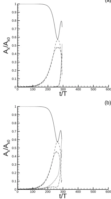
Figure 5 presents the evolution of components k0, k1, k2,
k3 and k4 propagated under wind action, in the same way
t/T
A
k/A
k0 0 100 200 300 400 500 600 0 0.1 0.2 0.3 0.4 0.5 0.6 0.7 0.8 0.9 1(a)
t/T
A
k/A
k0 0 100 200 300 400 500 600 0 0.1 0.2 0.3 0.4 0.5 0.6 0.7 0.8 0.9 1(b)
Fig. 5. Time evolution of the components of the
fundamen-tal mode k0=9 (solid line), of subharmonic modes k1=7 (dashed
line) and k3=8 (dotted line), and of superharmonic modes k4=10
(dash-dotted line) and k2=11 (dash-dot-doted line) propagated
un-der wind action. (a): From initial condition (1). (b): From initial condition (2).
it was done on Fig. 2 without wind. Curves last up to t /T =295, after numerical blow up. Results obtained from initial conditions (1) and (2) are very similar. One can no-tice that in both cases, components k1 and k2 are not
af-fected by the introduction of wind. Differences appear on the behavior of components k3 and k4. If components
re-lated to perturbation p seem to follow the evolution they had without wind, components related to perturbation q show a rapid divergence from their behavior without wind. By com-paring Fig. 2b and Fig. 5b, it appears that amplitude of the
128 J. Touboul: On the influence of wind on extreme wave events components k3and k4grow earlier in presence of wind. In
presence of wind, these components are dominant around t /T =290, while without wind, they are not dominant be-fore t /T =400. Between Figs. 2a and 5a, the difference is also very important. The normalized amplitude of compo-nents k3and k4, related to perturbation q, never exceeds 0.01
when propagated without wind. But while propagated un-der wind action, these components become dominant after t /T =290. As a matter of fact, the modulation q, which is not the most unstable, turns out to be more sensitive to wind forcing. This observation could be explained while noticing that a phase opposition exists between the two freak waves present around the time of maximum modulation. Therefore, the forcing criterion is not overcome simultaneously, but al-ternatively by these waves. This could result in the forc-ing of the perturbation q, which presents one wavelength in the computational domain, instead of perturbation p, which presents two.
5 Conclusions
The effect of wind on freak waves generated by means of modulational instability has been investigated numerically. Two initial conditions have been considered. In the first one, only the most linearly unstable perturbation has been consid-ered, while in the other one, the two perturbations linearly unstable were imposed. Those initial conditions have been propagated with, and without wind.
It appeared that without wind, the Fermi-Pasta-Ulam re-currence disappear when both modulations are present. This recurrence is broken by the presence of a second perturba-tion, of different growth rate. As a matter of fact, two cycle of different length are superimposed, and nonlinear interac-tions quickly destruct recurrence.
Under wind forcing, the lifetime of the freak wave is in-creased, in both cases. An amplification of the peak is also found, confirming previous results by Touboul and Kharif (2006). But in both cases, the influence of wind seems to help developing the perturbation which is not the most un-stable. In both simulations, wind forcing lead to numerical blow up, which is understood as wave breaking.
As a result, it appears that wind blowing over rogue waves lead them to breaking. Those waves, naturally dangerous, become very more devastating while breaking. The impact of huge breaking waves on ships or off-shore structures is re-sponsible of a large amount of energy destroying those struc-tures. This phenomenon appears to be supported by wind action on rogue waves.
To improve and validate this approach, a stronger inves-tigation of the pressure distribution in separating flows over waves is required. A two phase flow code is being developed for this study. A numerical simulation of the problem will provide a lot of information on the pressure distribution at the interface, and on the controling parameters.
Acknowledgements. The author would like to thank C. Kharif for very interesting and helpful conversations.
Edited by: E. Pelinovsky Reviewed by: two referees
References
Banner, M. I. and Melville, W. K.: On the separation of air flow over water waves, J. Fluid Mech., 77, 825–842, 1976.
Banner, M. I. and Tian, X.: On the separation of air flow over water waves, J. Fluid Mech., 367, 107–137, 1998.
Bliven, L. F., Huang, N. E., and Long, S. R.: Experimental study of the influence of wind on BenjaminFeir sideband, J. Fluid Mech., 162, 237–260, 1986.
Dias, F. and Kharif, C.: Nonlinear gravity and capillary-gravity waves, Annu. Rev. Fluid Mech., 31, 301–346, 1999.
Dommermuth, D. and Yue, D.: A high order spectral method for the study of nonlinear water waves, J. Fluid Mech., 184, 267– 288, 1987.
Giovanangeli, J. P., Touboul, J., and Kharif, C.: On the role of the Jeffreys’ sheltering mechanism in sustaining extreme water waves, C. R. Acad. Sci. Paris, Ser. IIB, 8-9, 568–573, 2006. Jeffreys, H.: On the formation of wave by wind, Proc. Roy. Soc. A,
107, 189–206, 1925.
Kharif, C. and Pelinovsky, E.: Physical mechanisms of the rogue wave phenomenon, Eur. J. Mech B/Fluids, 22, 603–634, 2003. Kharif, C. and Ramamonjiarisoa, A.: Deep water gravity wave
in-stabilities at large steepness, Phys. Fluids, 31, 1286–1288, 1988. Lawton, G.: Monsters of the deep (the perfect wave), New Scientist,
170(2297), 28–32, 2001.
Longuet-Higgins, M. S.: Bifurcation in gravity waves, J. Fluid Mech., 151, 457–475, 1985.
Mallory, J. K.: Abnormal waves on the South-East Africa, Int. Hy-drog. Rev., 51, 89–129, 1974.
McLean, J. W.: Instabilities of finite-amplitude water waves, J. Fluid Mech., 114, 315–330, 1982.
McLean, J. W., Ma, Y. C., Martin, D. U., Saffman, P. G., and Yuen, H. C.: Three-dimensional instability of finite-amplitude water waves, Phys. Rev. Lett., 46, 817–820, 1981.
Skandrani, C., Kharif, C., and Poitevin, J.: Nonlinear evolution of water surface waves: The frequency downshifting phenomenon, Contemp. Math., 200, 157–171, 1996.
Tanaka, M.: A method for studying nonlinear random field of sur-face gravity waves by direct numerical simulation, Fluid Dyn. Res., 28, 41–60, 2001.
Touboul, J. and Kharif, C.: On the interaction of wind and extreme gravity waves due to modulational instability, Phys. Fluids, 18, 108103, 2006.
Touboul, J., Giovanangeli, J. P., Kharif, C., and Pelinovsky, E.: Freak waves under the action of wind: experiments and simu-lations, Eur. J. Mech. B/Fluids, 25, 662–676, 2006.
Trulsen, K. and Dysthe, K. B.: Action of wind stress and break-ing on the evolution of a wave train, in: IUTAM Symposium on Breaking Waves, edited by: Grimshaw, B., pp. 243–249, Springer-Verlag, 1991.
West, B., Brueckner, K., Janda, R., Milder, M., and Milton, R.: A new numerical method for surface hydrodynamics, J. Geophys. Res., 92(C11), 11 803–11 824, 1987.