HAL Id: hal-00318001
https://hal.archives-ouvertes.fr/hal-00318001
Submitted on 22 Nov 2005
HAL is a multi-disciplinary open access
archive for the deposit and dissemination of
sci-entific research documents, whether they are
pub-lished or not. The documents may come from
teaching and research institutions in France or
abroad, or from public or private research centers.
L’archive ouverte pluridisciplinaire HAL, est
destinée au dépôt et à la diffusion de documents
scientifiques de niveau recherche, publiés ou non,
émanant des établissements d’enseignement et de
recherche français ou étrangers, des laboratoires
publics ou privés.
Predictions of local ground geomagnetic field
fluctuations during the 7-10 November 2004 events
studied with solar wind driven models
P. Wintoft, M. Wik, H. Lundstedt, L. Eliasson
To cite this version:
P. Wintoft, M. Wik, H. Lundstedt, L. Eliasson. Predictions of local ground geomagnetic field
fluc-tuations during the 7-10 November 2004 events studied with solar wind driven models. Annales
Geophysicae, European Geosciences Union, 2005, 23 (9), pp.3095-3101. �hal-00318001�
SRef-ID: 1432-0576/ag/2005-23-3095 © European Geosciences Union 2005
Annales
Geophysicae
Predictions of local ground geomagnetic field fluctuations during the
7–10 November 2004 events studied with solar wind driven models
P. Wintoft1, M. Wik1, H. Lundstedt1, and L. Eliasson2
1Swedish Institute of Space Physics, Lund, Sweden 2Swedish Institute of Space Physics, Kiruna, Sweden
Received: 22 February 2005 – Revised: 6 July 2005 – Accepted: 13 July 2005 – Published: 22 November 2005 Part of Special Issue “1st European Space Weather Week (ESWW)”
Abstract. The 7–10 November 2004 period contains two events for which the local ground magnetic field was severely disturbed and simultaneously, the solar wind displayed sev-eral shocks and negative Bzperiods. Using empirical models
the 10-min RMS 1X and 1Y at Brorfelde (BFE, 11.67◦E, 55.63◦N), Denmark, are predicted. The models are recur-rent neural networks with 10-min solar wind plasma and magnetic field data as inputs. The predictions show a good agreement during 7 November, up until around noon on 8 November, after which the predictions become significantly poorer. The correlations between observed and predicted log RMS 1X is 0.77 during 7–8 November but drops to 0.38 during 9–10 November. For RMS 1Y the correlations for the two periods are 0.71 and 0.41, respectively. Studying the solar wind data for other L1-spacecraft (WIND and SOHO) it seems that the ACE data have a better agreement to the near-Earth solar wind during the first two days as compared to the last two days. Thus, the accuracy of the predictions depends on the location of the spacecraft and the solar wind flow direction. Another finding, for the events studied here, is that the 1X and 1Y models showed a very different de-pendence on Bz. The 1X model is almost independent of
the solar wind magnetic field Bz, except at times when Bzis
exceptionally large or when the overall activity is low. On the contrary, the 1Y model shows a strong dependence on
Bzat all times.
Keywords. Magnetospheric physics (Solar wind-magnetosphere) – Geomagnetism and Paleomagnetism (Rapid time variations) – Ionosphere (Modeling and forecasting)
Correspondence to: P. Wintoft
1 Introduction
The Earth’s magnetosphere is a dynamic system that re-sponds to changes in the upstream solar wind. Through complex processes that includes magnetic reconnection and viscous instabilities, energy is transferred from the solar wind into the magnetosphere (Baumjohann and Haerendel, 1987), with subsequent energy dissipation through geomag-netic storms and substorms (Gonzalez et al., 1994). A major fraction of large geomagnetic storms is caused by coronal mass ejections (CME) (Gosling et al., 1991). The CME, and its interplanetary counterpart, the ICME, plows through the ambient solar wind, producing shock waves and following sheath regions (Owens et al., 2005). In some cases the ICME evolves as a magnetic cloud (Burlaga, 1995) with smooth magnetic field line rotation during which the Bzcomponent
may be strongly negative for an extended period of time, en-abling entry of solar wind energy through magnetic recon-nection. Another source for geomagnetic activity, especially during the declining phase of solar activity, is seen in high speed solar wind streams (Richardson et al., 2002). The dif-ferent structures interact and evolve as they travel from the Sun to the Earth, causing various degrees of geoeffectiveness (Huttunen et al., 2002; Echer and Gonzales, 2004).
During the geomagnetic storm, different current systems are modified, like the ionospheric currents, ring current, and magnetopause current. On the ground the currents are ob-served as deviations of the local geomagnetic field (Nishida, 1978). Several indices have been derived for various geo-physical phenomena (Mayaud, 1980) and their coupling to the solar wind have been extensively studied (Baker, 1986), and especially the Dst index (Wu and Lundstedt, 1997;
Kli-mas et al., 1998). The effects of geomagnetic disturbances are observed on technological systems, such as electrical power grids, pipe lines, and telegraph lines (Boteler et al., 1998, Lundstedt, 20041), and are called geomagnetically
1Lundstedt, H.: The Sun, Space Weather and GIC Effects in
3096 P. Wintoft et al.: Predictions of local ground geomagnetic field fluctuations induced currents (GIC). There is great interest in modelling
GIC, both for post-event analysis and for predictions. As a result there are three parallel GIC studies within the ESA Space Weather Applications Pilot Project and these can be found at the web page http://www.esa-spaceweather.net/.
The GIC can be estimated in different ways. One ap-proach is to use geomagnetic indices, as several can be suc-cessfully predicted: AE (Gleisner and Lundstedt, 2001a),
Dst (Vassiliadis and Klimas, 1999; Lundstedt et al., 2002),
and Kp (Boberg et al., 2000). The index is then translated
into a physical quantity that is related to GIC. Boteler (2001) showed that there is close to a linear relationship between the 3-h Kpindex and the logarithm of the ground electric field.
However, the indices have their limitations because they have been derived to capture some specific aspect of the mag-netospheric variation. Another approach is to use observed ground geomagnetic field data. The calculation of GIC can then be divided into two steps (Pirjola, 2002) involving a geo-physical part to determine the geoelectric field and an engi-neering part to compute the currents in the technological sys-tem. The electric field is computed from the magnetic field by assuming an equivalent ionospheric current system such that the geomagnetic variations at the Earth’s surface can be explained by horizontal divergence-free ionospheric currents (Viljanen et al., 2003). Solar wind–magnetosphere coupling models can then be used to predict the local ground magnetic field. In Gleisner and Lundstedt (2001b) a model was devel-oped that predicts the 10-min average local geomagnetic field using solar wind data. But, as the electric field is related to the rate-of-change of the magnetic field (dB/dt) via Fara-day’s law of induction ∇×E=−∂B∂t, a more basic quantity to use is the time difference of B, i.e. 1B(t)=B(t+1)−B(t ) (Viljanen et al., 2001). However, most of the power in 1B is located at small scales (high frequencies) and therefore a large fraction of the signal will be lost if 1B is temporally averaged, or if 1B is formed from a temporally averaged B (Wintoft, 2005). This happens already at 5 to 10 min aver-ages. Therefore, other moments of 1B should be consid-ered. In the work by Weigel et al. (2002) models were de-veloped that predict the average absolute value of 1B with a temporal resolution of 30 min. More specifically, they stud-ied the north-south component of the magnetic field, i.e.
h|1X|i30min. As the average is taken of the absolute value,
a large fraction of the variance from the original signal is maintained. The best model reached an overall prediction efficiency of 0.4 based on data from 1998–1999.
The models developed by Wintoft (2005) aims instead at predicting the 10-min root-mean-square (RMS) of 1X (and
1Y). The motivation of using RMS data is summarised here. The power spectrum of 1X peaks at small scales and de-creases quickly with increasing scale: 83% of the power is located at scales τ ≤8 min, 99% at τ ≤128 min. We speak in terms of scales as defined from wavelet analysis, but the scale may be translated into the approximate frequency band
[1/4τ, 1/2τ ] (Percival and Walden, 2002). One may also picture the signal at a certain scale as being the difference between two consecutive averages of width τ . It was found
that the RMS data can be used to estimate the power spectra of 1X and 1Y . This is useful for the subsequent analysis, for example, computing GIC, as both amplitude and scale (fre-quency) are available. Another issue is that the RMS data captures a major fraction of the variance in 1X. The relative variance is Var(RMS1X)/Var(1X)=0.82. For comparison the 10-min average absolute 1X has a relative variance of Var(h|1X|i)/Var(1X)=0.55. Finally, any temporal averag-ing will decrease the forecast lead time. To illustrate this we may consider a time dependent parameter x(t ) that is col-lected with a sampling interval 1t that results in the time series xi. The corresponding time stamp ti marks the
begin-ning of the interval so that xi is the average of x(t ) over the
interval t ∈[ti, ti+1], where ti+1=ti+1t. Similarly, we may
have another variable y(t ) sampled to yi. If we now wish
to develop a model that predicts y from x with lead time T we have ˆy(t +T )=f (x(t )), where ˆy is the prediction of y. This leads to the discrete model ˆyi+k=f (xi)where T =k1t.
Now assume that the current time is t0. The latest available
input is x−1and it has been collected over the time interval
[t−1, t0]. With a forecast time of T =k1t we will therefore
forecast yk−1, resulting in a true forecast time of T0=T −1t.
In order for the model to perform actual forecasts, we must have 1t≤T .
In this work we will use the previously developed mod-els to predict the disturbed period during 7 to 10 Novem-ber 2004. The following section describes the observed data, Sect. 3 describes the model, Sect. 4 address forecast errors related to the location of the solar wind monitor and the con-trol of the IMF Bzcomponent. In Sect. 5 the conclusions are
given.
2 The 7–10 November 2004 events
The 7–10 November 2004 period contains two events for which the local ground magnetic field was severely disturbed and the solar wind displays several shocks and negative Bz
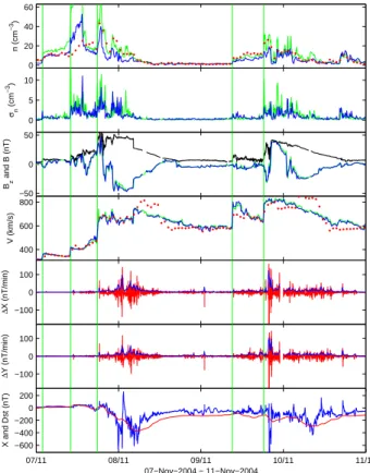
periods. In Fig. 1 the solar wind plasma and magnetic field data are shown, together with the ground magnetic field de-viations at Brorfelde (BFE, 11.67◦E, 55.63◦N). The
devia-tions are the one-minute differences of the north-south (X) and east-west (Y ) magnetic field components
1X(t ) = X(t +1) − X(t ), (1)
1Y (t ) = Y (t +1) − Y (t ), (2)
as approximations to dX/dt and dY /dt. The solar wind data comes from three spacecraft: ACE (blue line), WIND (green line), and SOHO (red dots). The ACE (Smith et al., 1998; McComas et al., 1998) and WIND (Ogilvie et al., 1995) data have been resampled to 10-min averages while the SOHO (Ipavich et al., 1998) data are one-hour averages. The four top panels show the particle density n, the standard deviation
σnof the density, the Bzmagnetic field component in GSM,
and the velocity V . The next two panels show the one-minute differences 1X and 1Y . The two panels also contain the
10-min root-mean-square (RMS) of 1X and 1Y . The bot-tom panel shows the north-south magnetic field X, minus 17 150 nT, and the Dst index. The five vertical lines
indi-cates the times of solar wind shocks. It is clear that these shocks are followed by sudden increases in |1X| and |1Y |. As the geomagnetic storm develops, large variations in 1X and 1Y are seen. During 8 November, the extreme values reach (1X, 1Y )=(140, 116) nT/min and during 9 Novem-ber (1X,1Y )=(−242, −229) nT/min. The corresponding 10-min RMS extreme values are (96,61) nT/min and (122, 104) nT/min, respectively. We also note that the ratio RMS1X/RMS1Y decreases from 1.6 for 8 November event to 1.2 for the 9 November event, indicating that the distur-bance is more along the north-south direction during the first event. These events have not yet been described in the scien-tific literature, however, a description can be found at Space Environment Center (http://www.sec.noaa.gov/weekly/).
We see that the Sun was very active with several CMEs. The first shock in early 7 November was probably caused by a CME on 3 November. There was a small increase in the so-lar wind magnetic field with a negative Bzcomponent. Both
1Xand 1Y display an impulse 66 min later in accordance with the ACE-magnetopause travel time of tACE=68 min at
the velocity of 365 km/s. The second shock, caused by a CME on 4 November was accompanied with larger increases in particle density n, σn, and B. Bz turned initially
north-ward and later southnorth-ward. The shock was followed by a magnetic impulse 55 min later, again in agreement with the 420 km/s velocity (tACE=59 min). Both 1X and 1Y
con-tinued to be slightly disturbed and Dst showed a weak
in-crease followed by a weak dein-crease typical for the magnetic storm initial and main phases. At the third shock the velocity jumped from 500 km/s to above 650 km/s, the magnetic field increased to almost 50 nT and Bzturned initially northward
and later strongly southward for an extended period of time. The source for this event was probably a series of CMEs that occurred late on 4 and early 6 November. The magnetic im-pulse took place 33 minutes later, in good agreement with a velocity of 650 km/s (tACE=38 min). The disturbed
pe-riod continued for about 19 h and Dst reached −373 nT on
8 November. What looks like a magnetic impulse early in 9 November is most likely a spurious value, as there are data gaps around that point and other stations show no such fea-ture. The fourth shock, around noon on 9 November shows quite different velocities for ACE/WIND and SOHO. The magnetic impulse occurs 16 min after the shock and is simi-lar in strength to that after the second shock. With a velocity of VACE=790 km/s there should be a delay of tACE=32 min.
It is thus difficult to associate this magnetic impulse with the measured solar wind at ACE. The fourth shock shows a jump in velocity from 650 km/s to 800 km/s and a magnetic im-pulse follows 29 min later, in agreement with tACE=31 min.
0 20 40 60 n (cm −3 ) 0 5 10 σn (cm − 3) −50 0 50 Bz and B (nT) 400 600 800 V (km/s) −100 0 100 ∆ X (nT/min) −100 0 100 ∆ Y (nT/min) 07/11 08/11 09/11 10/11 11/11 −600 −400 −200 0 200 07−Nov−2004 − 11−Nov−2004 X and Dst (nT)
Fig. 1. The panels show, from top to bottom: solar wind density
n(ACE–blue, WIND–green, SOHO–red), standard deviation σnof
the density, Bzmagnetic field component in GSM and total field B
from ACE (black), velocity V , one-minute 1X (red) and 10-min RMS 1X (blue), one-minute 1Y and 10-min RMS 1Y , and one minute X (blue) and hourly Dst (red). The period extends over the
four days of 7–10 November 2004. The only available data from SOHO are the hourly average density and velocity.
3 Forecasting RMS (1X,1Y ) using ACE
The empirical models previously developed predict the 10-min RMS 1X and 1Y for southern Scandinavia, with a pre-diction lead time of 30 min (Wintoft, 2005). The models are recurrent neural networks with solar wind plasma and mag-netic field data as inputs: 10-min averages of magmag-netic field
Bz, particle density n, velocity V , and standard deviations
(σ ) of the same parameters. Local time and time of year were also used.
The models were trained and validated on data from the six year period 1998–2003. As the distributions of RMS 1X and 1Y are dominated by values close to zero only a selected subset was used, in order to avoid the network becoming biased towards quiet conditions. However, large values are still typically underestimated, as they are more infrequent. The prediction horizon of 30 min was selected to enable the models to predict events with a large range of solar wind ve-locities. A velocity of 830 km/s at L1 takes 30 min to reach the magnetopause. We also studied models where the pre-diction lead time was increased up to 90 min, but for both
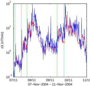
3098 P. Wintoft et al.: Predictions of local ground geomagnetic field fluctuations 07/11 08/11 09/11 10/11 11/11 10−1 100 101 102 07−Nov−2004 − 11−Nov−2004 ∆ X (nT/min)
Fig. 2. The figure shows the observed (blue) and predicted (red) 10-min RMS 1X.
networks were trained and the optimal models gave a cor-relation of 0.79 and prediction efficiency (Detman and Vas-siliadis, 1997) of 0.63 of the logarithm of the RMS data. It is important to notice here that the geomagnetic data are not used as input to the model, only solar wind data, otherwise the correlation could be even higher but not necessarily truly improving the predictions. For example, a simple persis-tence model, predicting RMS 1X(t +30 min) based on RMS
1X(t ), would have a correlation of 0.72 but the predictions would consistently lag by 30 min. To verify that the solar wind–1X model is actually making 30 min forecasts, with the stated correlation, we may compute the correlation coef-ficient between the observed 1X and the predicted 1X by shifting the predicted 1X backwards and forwards in time. For a true forecast the maximum correlation should occur at 30 min and decrease for smaller and larger prediction times, and this is also the case for the neural network models.
It was shown that the solar wind influence on 1X and
1Y were slightly different. The most important inputs for
1X, in order of increasing importance, were local time, Bz,
σn, and V . For 1Y it was local time, σn, V , and Bz. The
other inputs, and mots notably n, had no significant influ-ence. The independence of n was also shown by Weigel et al. (2002). The models have been implemented for real time operation and the forecasts are displayed on a web page (http://www.lund.irf.se/gicpilot/gicforecastprototype/). The predictions of RMS 1X and 1Y for the November events are shown in Figs. 2 and 3. It is seen that the predictions cap-ture the large-scale variations but not the sample-to-sample variations. The predictions show a good agreement during 7 November, up until around noon on 8 November, after which the predictions become significantly poorer. The correlations between observed and predicted log RMS 1X is 0.77 during
07/11 08/11 09/11 10/11 11/11 10−1 100 101 102 07−Nov−2004 − 11−Nov−2004 ∆ Y (nT/min)
Fig. 3. The figure shows the observed (blue) and predicted (red) 10-min RMS 1Y .
7–8 November but drops to 0.38 during 9–10 November. For RMS 1Y the correlation for the two periods are 0.71 and 0.41, respectively.
4 Discussion
In the following sections we address the forecast quality in relation to the location of the solar wind monitor and study the coupling to the solar wind Bzcomponent.
4.1 The locations of solar wind monitors
The ACE spacecraft is in orbit around L1 approximately 240 Earth radii (RE) upstream from Earth. Due to the large
dis-tance there may be considerable differences in solar wind properties at ACE and close to Earth. In the study by Dalin et al. (2002) it was shown that the correlation of solar wind plasma data from different spacecraft could, at times, be small and the correlation decreased with increasing (Y,Z)-separation. For the period studied here the ACE spacecraft is located approximately at (X,Y,Z)=(242, 23, −15) REin GSE
coordinate system. Two other spacecraft are also located around L1, namely SOHO at (218, −104, −3) REand WIND
at (199, 59, −9) RE. The spacecraft are almost located in the
(X,Y)-plane, with the largest separation of 12 RE in the
Z-direction. However, in the Y-direction the distance is as large as 163 RE. In the X-direction the separation is about 42 RE,
and with a velocity of 400 km/s or higher the separation in time is less than 11 minutes. From Fig. 1 we see that the
Bzmagnetic field components for ACE and WIND are very
well correlated. There is a shift of <10 min, barely visible in the figure, that comes from the separation in X. Studying the velocity, there is again a very good agreement between ACE
−150 −100 −50 0 50 100 150 −150 −100 −50 0 50 100 150 2004−11−07 2004−11−08 2004−11−09 2004−11−10
WIND ACE SOHO
Y (R
E)
Z (R
E
)
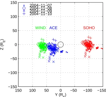
Fig. 4. The figure shows the advected spacecraft locations onto the plane X=10 REusing hourly average velocity vectors from WIND.
The data have been divided into the four days: 7 November (dots), 8 November (diamonds), 9 November (crosses), and 10 November (pluses). The black circle is centred on Earth and has a radius of 10 RE.
and WIND. The hourly average SOHO velocity data show a good agreement during 7 November, up to 05:00 UT on 8 November, despite its large distance from ACE and WIND. After that, the SOHO velocity deviates significantly most of the time. It thus seems that the velocity structure is ho-mogenous at the beginning of the period and then becomes more fragmented. The ACE and WIND densities show sim-ilar temporal variation, although WIND mostly gives higher densities, often by a factor 2 to 3. Except for the first part of 7 November, the SOHO density agrees quite well with the WIND density.
In Fig. 4 the crossing of the solar wind in the (Y, Z)-plane at X=10 RE(typical megnetopause distance) is shown for the
three spacecraft. As we only have all three velocity com-ponents for WIND, we have assumed the same velocity for the three spacecraft. The circle in the centre has a radius of 10 RE. We see that the measurements at ACE advected to
X=10 come reasonably close to the Earth during 7 Novem-ber (dots). The most distant points are the two westerly dots, but simultaneously the WIND measurements come close to the Earth, and as ACE and WIND show a very good agree-ment for the whole period, we may conclude that the mea-surements at ACE depicts quite well what the solar wind is like close to the Earth during 7 November. Then, during 8 November, the advected location of ACE (diamonds) moves towards the east and south. During this day the velocities at SOHO and ACE also start to deviate. Then, during 9 Novem-ber, the advected ACE location turns far south (crosses) of the Earth. It is thus possible that the measurements at ACE from the morning of 8 November through 9 November do
−50 0 50 B z (nT) 100 101 RMS ∆ X 07/11 08/11 09/11 10/11 11/11 100 101 RMS ∆ Y
Fig. 5. The three panels show, from top to bottom: solar wind Bz
(blue) and −Bz(red), predicted RMS 1X using Bz(blue) and −Bz
(red), and predicted RMS 1Y using Bz(blue) and −Bz(red).
not represent accurately the solar wind close to the Earth. Turning back to the predictions shown in Figs. 2 and 3, it was seen that the correlation was higher during the first two days as compared to the last two days. Thus, this may be the result that the solar wind at ACE correlates well with the solar wind close to the Earth in the early part of the period but not later in the period. The errors are particularly large during the late evening to midnight on 9 November. Study-ing another model that predicts the geomagnetic index Dst
(Lundstedt et al., 2002), also using ACE data as input, re-veals that the prediction errors are large for the same hours. 4.2 The influence of Bz
Using the prediction models the influence of the solar wind on RMS 1X and 1Y may be studied. In principal, some interesting artificial values could be selected to represent the solar wind to study the response of the model. However, care has to be taken so that the data represent a valid physical and statistical configuration, otherwise the output from the model will not be correct. One parameter that can be easily studied is Bz. It is perfectly valid to change the sign on Bzand run
the models, as we expect that the direction of B is not corre-lated with density or velocity. For example, a magnetic cloud starts with a simultaneous increase in n, V , and B (Burlaga, 1995). But Bzmay initially either turn northward or
south-ward, with the subsequent evolution determined by the cloud topology. The result is shown in Fig. 5. The blue curve rep-resents the original Bz and the red curve −Bz (top panel).
The model outputs are shown accordingly, in blue and red (bottom panels). The first apparent observation is that RMS
1Xshows a weak coupling to Bz, as changing the sign has
very little effect on the output. On the contrary, RMS 1Y is much more affected.
3100 P. Wintoft et al.: Predictions of local ground geomagnetic field fluctuations Looking at the details we note that the variations in the two
predictions of RMS 1X are very similar up to 23:00 UT on 7 November, even though the sign on Bzhas been changed.
During the following hours, when Bzis strongly negative, up
to 05:00 UT on 8 November there is a difference of about a factor 2. Then, the predictions coincide again when Bzgoes
towards zeros and the velocity decreases. But then, during a period of low activity from 12:00 UT on 8 November to 09:00 UT on 9 November, when Bzis close to zero, there is
again a difference of a factor 2, with slightly higher activity when Bzis negative.
5 Conclusions
In this work we have studied the prediction of the 10-min variation of the local ground magnetic field, more specifi-cally, the 10-min RMS 1X and 1Y . The prediction model uses the solar wind data from the ACE spacecraft. The four-day period extending over 7 November to 10 November 2004 was explored.
It was found that the sample-to-sample variations in RMS
1Xand 1Y are not predicted, but the large-scale variations are predicted. The predictions of the first two days show a higher correlation with the observations than during the last two days. By studying the solar wind data for other L1-spacecraft (WIND and SOHO), it seems that the ACE data have a better agreement to the near-Earth solar wind during the first two days as compared to the last two days. In a study by Dalin et al. (2002) it was also shown that the correlation of solar wind plasma data from different spacecraft decreased with increasing (Y, Z)-separation. Thus, the accuracy of the predictions depends on the location of the spacecraft and the solar wind flow direction.
The models have not been developed to predict the re-sponse of 1X or 1Y for specific solar wind structures; the only criterion used on the data selection is that there should be contiguous data for 48 h, or longer, for which RMS
>10 nT/min at least once. This means that solitary peaks in RMS 1X or 1Y will be difficult to model because of the low relative occurrence rate. However, the peaks may also be related to magnetic impulse events (Kataoka et al., 2003) that show a significant correlation to discontinuities of the in-terplanetary magnetic field, and not Bz, therefore, additional
inputs should be considered in future studies.
By modifying the solar wind input data the response of the model may be studied. Care has to be taken in how the input is modified, but a valid modification from a physical and statistical point of view is to change the sign of Bz. It
was found, for the events studied here, that the 1X and 1Y models showed a very different dependence on Bz. The 1X
model is almost independent of the solar wind magnetic field
Bz, except at times when Bzis large or when the overall
ac-tivity is low. On the contrary, the 1Y model shows a strong dependence on Bzat all times.
In the models developed by Wintoft (2005) the location of ACE was not considered. Thus, it is reasonable to believe
that there are data in the solar wind data set used for model development that are poorly correlated to the near-Earth solar wind. The inclusion of such data during the model develop-ment has the effect of increased noise. In future work, a more careful selection of data, taking into account the location of ACE, should be considered.
Acknowledgements. We are grateful to the providers of the solar
wind and ground magnetic field data: ACE data from CalTech and SEC; the MIT Space Plasma Group for the WIND plasma data and NASA/GSFC for the WIND magnetic field data; the University of Maryland for the SOHO/PM data; the Solar-Terrestrial Physics Di-vision at the Danish Meteorological Institute for the Brorfelde mag-netic field data. COST 724 is acknowledged for financial support. This work has been carried out with support from ESA/ESTEC (Contract No. 16953/02/NL/LvH).
Topical Editor T. Pulkkinen thanks J. B. Blake and another ref-eree for their help in evaluating this paper.
References
Baker, D. N.: Statistical analyses in the study of solar wind-magnetosphere coupling, Solar Wind-Magnetosphere Coupling, 17–38, 1986.
Baumjohann, W. and Haerendel, G.: Entry and dissipation of en-ergy in the Earth’s magnetosphere, in Space Astronomy and So-lar System Exploration: Proceeding of summer school held at aplbach, Austria, 29 July–8 August, 1986, 121–130, ESA, 1987. Boberg, F., Wintoft, P., and Lundstedt, H.: Real time Kp
predic-tions from solar wind data using neural networks, Physics and Chemistry of the Earth, 25, 275–280, 2000.
Boteler, D.: Assessment of geomagnetic hazards to power systems in Canada, Natural Hazards, 23, 101–120, 2001.
Boteler, D. H., Pirjola, R. J., and Nevanlinna, H.: The effects of ge-omagnetic disturbances on electrical systems at the Earth’s sur-face, Adv. Space Res., 22, 17–27, 1998.
Burlaga, L. F.: Interplanetary magnetohydrodynamics, Oxford Uni-versity Press, 1995.
Dalin, P., Zastenker, G., Paularena, K., and Richardson, J.: The main features of solar wind plasma correlations of importance to space weather strategy, J. Atmos. S.-P., 64, 737–742, 2002. Detman, T. R. and Vassiliadis, D.: Review of techniques for
mag-netic storm forecasting, 253–266, AGU, 1997.
Echer, E. and Gonzales, W. D.: Geoeffectiveness of interplanetary shocks, magnetic clouds, sector boundary crossings and their combined occurrence, Geophys. Res. Lett., 31, L09 808, 2004. Gleisner, H. and Lundstedt, H.: Auroral electrojet predictions with
dynamic neural networks, J. Geophys. Res., 106, 24 541–24 550, 2001a.
Gleisner, H. and Lundstedt, H.: Neural network-based local model for prediction of geomagnetic disturbances, J. Geophys. Res., 106, 8425–8433, 2001b.
Gonzalez, W. D., Joselyn, J. A., Kamide, Y., Kroehl, H. W., Ros-toker, G., Tsurutani, B. T., and Vasyliunas, V. M.: What is a geomagnetic storm?, J. Geophys. Res., 99, 5771–5792, 1994. Gosling, J. T., McComas, D. J., Phillips, J. L., and Bame, S. J.:
Geo-magnetic activity associated with Earth passage of interplanetary shock disturbances and coronal mass ejections, J. Geophys. Res., 96, 7831–7839, 1991.
Huttunen, K. E. J., Koskinen, H. E. J., and Schwenn, R.: Variability of magnetospheric storms driven by different solar wind pertu-bations, J. Geophys. Res., 107, SMP 20–1–8, 2002.
Ipavich, F. M., Galvin, A. B., Lasley, S. E., Paquette, J. A., Hefti, S., Reiche, K., Coplan, M. A., Gloeckler, G., Bochsler, P., Hov-estadt, D., Gr¨unwaldt, H., Hilchenbach, M., et al.: Solar wind measurements with SOHO: The CELIAS/MTOF proton moni-tor, J. Geophys. Res., 103, 17 205–17 213, 1998.
Kataoka, R., Fukunishi, H., and Lanzerotti, L. J.: Statistical iden-tification of solar wind origins of magnetic impulsive events, J. Geophys. Res., 108, SMP 13–1–12, 2003.
Klimas, A. J., Vassiliadis, D., and Baker, D. N.: Dst index
predic-tion using data-derived analogues of the magnetospheric dynam-ics, J. Geophys. Res., 103, 20 435–20 448, 1998.
Lundstedt, H., Gleisner, H., and Wintoft, P.: Operational forecasts of the geomagnetic Dst index, Geophys. Res. Lett., 29, 34–1– 34–4, 2002.
Mayaud, P. N.: Derivation, meaning, and use of geomagnetic in-dices, Geophysical Monograph Series, AGU, 1980.
McComas, D. J., Bame, S. J., Barker, P., Feldman, W. C., Phillips, J. L., Riley, P., and Griffee, J. W.: Solar wind electron proton alpha monitor (SWEPAM) for the Advanced Composition Ex-plorer, Space Science Reviews, 86, 563–612, 1998.
Nishida, A.: Geomagnetic Diagnosis of the Magnetosphere, 9 of Physics and Chemistry in Space, Springer-Verlag, 1978. Ogilvie, K. W., Chornay, D. J., Fritzenreiter, R. J., Hunsaker, F.,
Keller, J., Lobell, J., Miller, G., Scudder, J. D., Sittler, Jr., E. C., Torbert, R. B., Bodet, D., Needell, G., Lazarus, A. J., et al.: SWE, a comprehensive plasma instrument for the WIND space-craft, Sp. Sc. R., 71, 55–77, 1995.
Owens, M. J., Cargill, P. J., Pagel, C., Siscoe, G. L., and Crooker, N. U.: Characteristic magnetic field and speed properties of in-terplanetary coronal mass ejections and their sheath regions, J. Geophys. Res., 110(A01), 105, 2005.
Percival, D. B. and Walden, A. T.: Wavelet methods for time series analysis, Cambridge University Press, 2002.
Pirjola, R.: Review on the calculation of surface electric and mag-netic fields and of geomagmag-netically induced currents in ground-based technological systems, Surv. Geophys., 23, 71–90, 2002. Richardson, I. G., Cane, H. V., and Cliver, E. W.: Sources of
ge-omagnetic activity during nearly three solar cycles, J. Geophys. Res., 107, SSH 8–1–13, 2002.
Smith, C. W., L’Heureux, J., Ness, N. F., Acu˜na, M. H., Burlaga, L. F., and Scheifele, J.: The ACE magnetic fields experiment, Space Sci. R., 86, 613–632, 1998.
Vassiliadis, D. and Klimas, A. J.: The Dstgeomagnetic response
as a function of storm phase and amplitude and the solar wind electric field, J. Geophys. Res., 104, 24 957–24 976, 1999. Viljanen, A., Nevanlinna, H., Pajunp¨a¨a, K., and Pulkkinen, A.:
Time derivate of the horizontal geomagnetic field as an activ-ity indicator, Ann. Geophys., 19, 1107–1118, 2001,
SRef-ID: 1432-0576/ag/2001-19-1107.
Viljanen, A., Pulkkinen, A., Amm, O., Pirjola, R., Korja, T., and BEAR Working Group: Fast computation of the geoelctric field using the method of elementary current systems and planar Earth models, Ann. Geophys., 22, 101–113, 2004,
SRef-ID: 1432-0576/ag/2004-22-101.
Weigel, R. S., Vassiliadis, D., and Klimas, A. J.: Coupling of the solar wind to temporal fluctuations in ground magnetic fields, Geophys. Res. Lett., 29, 2002.
Wintoft, P.: Study of the Solar Wind Coupling to the Time Differ-ence Horizontal Geomagnetic Field, Ann. Geophys., 23, 1949– 1957, 2005,
SRef-ID: 1432-0576/ag/2005-23-1949.
Wu, J.-G. and Lundstedt, H.: Neural network modeling of solar wind–magnetosphere interaction, J. Geophys. Res., 102, 14 457– 14 466, 1997.