Unsupervised classification of saturated areas using a time series of remotely sensed images

(1)

HAL Id: hal-00298847

https://hal.archives-ouvertes.fr/hal-00298847

Submitted on 15 Jun 2007

HAL is a multi-disciplinary open access

archive for the deposit and dissemination of sci-entific research documents, whether they are pub-lished or not. The documents may come from teaching and research institutions in France or abroad, or from public or private research centers.

L’archive ouverte pluridisciplinaire HAL, est destinée au dépôt et à la diffusion de documents scientifiques de niveau recherche, publiés ou non, émanant des établissements d’enseignement et de recherche français ou étrangers, des laboratoires publics ou privés.

Unsupervised classification of saturated areas using a

time series of remotely sensed images

D. A. Dealwis, Z. M. Easton, H. E. Dahlke, W. D. Philpot, T. S. Steenhuis

To cite this version:

D. A. Dealwis, Z. M. Easton, H. E. Dahlke, W. D. Philpot, T. S. Steenhuis. Unsupervised classification of saturated areas using a time series of remotely sensed images. Hydrology and Earth System Sciences Discussions, European Geosciences Union, 2007, 4 (3), pp.1663-1696. �hal-00298847�

(2)

HESSD

4, 1663–1696, 2007

Using and NDWI to delineate saturated areas D. A. DeAlwis et al. Title Page Abstract Introduction Conclusions References Tables Figures ◭ ◮ ◭ ◮ Back Close

Full Screen / Esc

Printer-friendly Version

Interactive Discussion

Hydrol. Earth Syst. Sci. Discuss., 4, 1663–1696, 2007 www.hydrol-earth-syst-sci-discuss.net/4/1663/2007/ © Author(s) 2007. This work is licensed

under a Creative Commons License.

Hydrology and Earth System Sciences Discussions

Papers published in Hydrology and Earth System Sciences Discussions are under open-access review for the journal Hydrology and Earth System Sciences

Unsupervised classification of saturated

areas using a time series of remotely

sensed images

D. A. DeAlwis1, Z. M. Easton1, H. E. Dahlke1, W. D. Philpot2, and T. S. Steenhuis1

1

Department of Biological and Environmental Engineering, Riley-Robb Hall, Cornell University, Ithaca, NY 14853, USA

2

School of Civil and Environmental Engineering, Hollister Hall, Cornell University, Ithaca, NY 14853, USA

Received: 24 May 2007 – Accepted: 30 May 2007 – Published: 15 June 2007 Correspondence to: T. S. Steenhuis (tss1@cornell.edu)

(3)

HESSD

4, 1663–1696, 2007

Full Screen / Esc

EGU Abstract

The spatial distribution of saturated areas is an important consideration in numerous applications, such as water resource planning or sighting of management practices. However, in humid well vegetated climates where runoff is produced by saturation ex-cess proex-cesses on hydrologically active areas (HAA) the delineation of these areas can

5

be difficult and time consuming. Much of the non-point source pollution in these wa-tersheds originates from these HAAs. Thus, a technique that can simply and reliably predict these areas would be a powerful tool for scientists and watershed managers tasked with implementing practices to improve water quality. Remotely sensed data is a source of spatial information and could be used to identify HAAs, should a proper

10

technique be developed. The objective of this study is to develop a methodology to determine the spatial variability of saturated areas using a temporal sequence of re-motely sensed images. The Normalized Difference Water Index (NDWI) was derived from medium resolution LANDSAT 7 ETM+ imagery collected over seven months in the Town Brook watershed in the Catskill Mountains of New York State and used to

15

characterize the areas that were susceptible to saturation. We found that within a sin-gle landcover type, saturated areas were characterized by the soil surface water con-tent when the vegetation was dormant and leaf water concon-tent of vegetation during the growing season. The resulting HAA map agreed well with both observed and spatially distributed computer simulated saturated areas. This methodology appears promising

20

for delineating saturated areas in the landscape.

1 Introduction

Information on the spatial and temporal distribution of soil moisture is an important pa-rameter to correctly characterize. Numerous applications rely on information about soil moisture levels, from hydrologic and climate models to techniques aimed at optimizing

25

(4)

HESSD

4, 1663–1696, 2007

Full Screen / Esc

can be used to obtain the spatial distribution of the soil moisture content over large areas, thus reducing expensive and time consuming field measurements.

In the Northeast United States there is great interest in delineating saturated areas that contribute surface runoff and non point source pollutant loads to surface waters. Once these areas are identified, management practices can be developed and

imple-5

mented to control pollution. The highly permeable surface soils underlain by a dense layer of glacial till cause the majority of the runoff to be produced in areas of the land-scape that become saturated either when rainfall exceeds potential evaporation over an extended time or when the groundwater table intersects the soil surface. These saturated or Hydrologically Active Areas (HAA) expand and contract during the course

10

of the year (Dunne and Black, 1970; Dunne and Leopold, 1978; Beven, 2001; Needle-man et al., 2004). Thus, remotely sensed observations have the potential of defining the saturated areas in the landscape.

One way of determining soil moisture contents from remotely sensed data is by us-ing the thermal emissions from soils in the microwave range, generally sensitive to

15

moisture variations in the top five cm of the soil (Guha and Lakshmi, 2002). Saturated surfaces emit low levels of microwave radiation, whereas dry soils emit much higher levels of microwave radiation (Wang and Schmugge, 1980). However, in many applica-tions it is difficult to separate the microwave signal from saturated and unsaturated soil due to competing effects of moisture content, surface roughness, vegetation, liquid

pre-20

cipitation, and complex topography unless the variables are known a priori (Schmugge, 1985; Bindlish et al., 2003). Hence, an extensive amount of calibration is necessary to fit the parameters and prior knowledge of the surface cover and state must be known (Kerr, 2007). Indeed, Wagner et al. (2007) state that microwave remote sensing sys-tems can capture the general trends in surface soil moisture conditions, but cannot be

25

used to estimate absolute soil moisture values.

A more promising approach to obtain soil moisture variability is to remotely sense the greenness variations of biomass within an otherwise homogeneous canopy (Yang et al., 2006), because variations in soil water directly affect the growth patterns of

(5)

HESSD

4, 1663–1696, 2007

Full Screen / Esc

EGU

the overlying vegetation. For example, in Kansas, Wang et al. (2001) observed that soil moisture affected remotely sensed Normalized Difference Vegetation Index (NDVI) greenness patterns in the Konza Prairie. Vegetation indices such as the NDVI make use of the contrast between the strong reflection of vegetation in the near infra-red (NIR) and the strong absorption by chlorophyll in the red (R) (Gates et al., 1965).

How-5

ever, one of the disadvantages of the vegetation indices is that they are only sensitive to biomass in the early growth stages when the leaf area index is less than three (Co-hen et al., 2003; Friedl et al., 1994; Law and Waring, 1994; C(Co-hen and Chilar; Co(Co-hen et al., 2003; Fassnacht et al., 1997). Above three, there is no clear relationship be-tween biomass and vegetation indices (Fassnacht et al., 1997; Killelea, 2005). Another

10

potential disadvantage when relating moisture content and vegetation indices is that vegetation growth is dependent upon a number of environmental factors, such as nu-trient availability, disease pressure, insect infestation, temperature, wind, soil moisture content, and relative humidity among others. Thus, it is important not to misinterpret changes in vegetation growth patterns as related solely to soil wetness. Nonetheless,

15

there is clear evidence that hydrologic properties can have a strong effect on vegetation growth (De Jong et al., 1984; Farrar et al., 1994; Nicholson and Farrar, 1994; Timlin et al., 2001).

Similar to vegetation indices but more sensitive to moisture contents at the near sur-face are indices using measurements in the short-wave infrared (SWIR) band, where

20

strong water absorption bands are centered around 1450, 1500 and 1950 nm (Karnieli et al., 2001). Since virtually no light penetrates the atmosphere near the center of these bands, the bands selected for satellite sensors are typically chosen to avoid them. However, the absorption bands are quite broad, and still have an effect well away from the center wavelengths. The feasibility of using the SWIR bands was first

25

suggested by Tucker (1980) who noted that LANDSAT 7 ETM+ Band 5, and the SWIR band of MODIS (1550 to 1750 nm) would be well suited for remote sensing of the plant canopy water content. While this band will also be sensitive to variations in atmospheric water vapor, over relatively small areas and on clear days, the atmospheric variability

(6)

HESSD

4, 1663–1696, 2007

Full Screen / Esc

will generally be negligible and the local variations will be related to the presence of water on the land surface. In vegetated areas, absorption by leaf water occurs in the SWIR and the reflectance from plants thereby is negatively related to the leaf water content (Bowman, 1989; Ceccato, et al., 2001; Hunt, et al., 1987; Tucker, 1980). In the absence of vegetative cover, the local variations in LANDSAT 7 ETM+ Band 5

re-5

flectance will be sensitive to changes in the surface (near surface) soil moisture content (Whiting et al., 2004; Xiao et al., 2002), while for plants it will sense the water content in the vegetation.

Variations in reflectance may also occur due to variations in internal leaf structure, leaf dry matter content (Fensholt, 2004), soil mineral composition, and organic matter

10

content (Whiting et al., 2004). Consequently, LANDSAT 7 ETM+ Band 5 reflectance values alone are not suitable for retrieving vegetation water content. In the NIR (LAND-SAT 7 ETM+ Band 4, 780 - 900 nm), well away from the water absorption band, re-flectance is influenced most by the same factors affecting the LANDSAT 7 ETM+ Band 5 or SWIR band (e.g. leaf internal structure and leaf dry matter content), but not by

15

water content (Fensholt, 2004). By considering information from both the LANDSAT 7 ETM+ Bands 4 and 5 we can obtain a better estimate of the true moisture status. The Normalized Difference Water Index, NDWI, (Gao, 1996) has been proposed to exploit this characteristic of Bands 4 and 5. Another advantage of using NDWI, as opposed to the NDVI, is that saturation does not occur until LAI six or greater (Fensholt, 2004).

20

Once the values for NDWI are obtained, there are two approaches to aggregating pixels into homogeneous regions of wetness behavior: supervised and unsupervised classification. Supervised classification relies on the expertise of the analyst to define training sites using prior knowledge of the site but can be labor intensive (Foody and Arora, 1996). In unsupervised classification, pixels that exhibit similar characteristics

25

are subdivided into homogeneous spectral regions based on a set of boundary condi-tions specified by the user (Le Hgarat-Mascle et al., 1997). Once the homogeneous regions are classified, knowledge of the area under study is needed to assign the correct wetness index to each region. Thus, both supervised and unsupervised

(7)

classi-HESSD

4, 1663–1696, 2007

Full Screen / Esc

EGU

fications require the user to possess knowledge of the study area in order to complete the classification. However, the clustering portion of unsupervised classification oper-ates without a priori information of the wetness index classification and groups samples based on the inherent similarity of individual spectral signals.

The objective of this study is to test the ability of remote sensing techniques,

specifi-5

cally the NDWI derived from LANDSAT 7 ETM+ measurements for obtaining the spatial distribution of frequently saturated areas in the landscape that contribute the majority of the runoff and thus pollutants during storm events. We first separate the landscape into different land cover types and then relate the temporal NDWI pattern within each landcover type to the soil moisture status. We hypothesize that areas of the landscape

10

prone to saturated conditions will exhibit higher NDWI in the spring, particularly follow-ing snowmelt. These areas typically have less soil storage capacity, and drain large areas making them saturate more frequently. Thus during the typically drier summer months we expect these areas to dry out more rapidly due to the lower soil storage capacity, and maintain a lower NDWI than areas of the landscape more conducive to

15

plant growth (i.e., areas with greater soil storage capacity and more plant available wa-ter). We then assess the accuracy of the NDWI predictions using several techniques, including ground truth data collected in the watershed, as well as by comparison with two distributed hydrologic models.

2 Methods

20

2.1 Study site

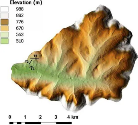
The site for this study was the Town Brook watershed (Fig. 1), in the Catskill Mountain region in New York State. The Town Brook watershed has an area of 37 km2 and an elevation range of 493 to 989 m (Fig. 2). The underlying geology of the watershed was formed during the glacial period, the north facing slopes are generally steep with

25

(8)

HESSD

4, 1663–1696, 2007

Full Screen / Esc

deciduous and evergreen forests. The south facing slopes are gentler with deeper soils particularly in the lower slope regions and are covered by shrubs, pastures, alfalfa, and corn grown in rotation. As mentioned above the hydrology is such that in late fall, winter, and early spring saturated areas develop mostly in the lower areas of the watershed on concave slopes and at locations where the slope flattens and thus the hydraulic

5

gradient is reduced. 2.2 Satellite images

A time sequence of multi-spectral LANDSAT 7 ETM+ images was used to identify spa-tial/temporal changes in the vegetative cover of Town Brook. The LANDSAT 7 ETM+ creates images with 30 m×30 m pixel size. The satellite orbital profile operates on a

16-10

day cycle, thus providing imagery every 16 days, each image covering a swath 183 km wide. The spectral range of Band 4 is 780–900 µ, and is primarily used to estimate biomass, although it can also discriminate water bodies, and soil moisture from veg-etation. Band 5 has a spectral range of 1550–1750 µ, and is particularly responsive variations in biomass and moisture. Seven cloud-free images were obtained on the

15

following dates: 27 January 2000, 5 April 2001, 7 May 2001, 8 June 2001, 10 July 2001, 12September 2001 and 30 October 2001. The vegetation and water indices calculated from these images are dependent on precipitation and snow cover on the ground. When the January 2000 image was taken there was snow on the ground. Dur-ing the rest of the acquisition period in 2001 there was 85 cm of precipitation, which

20

is below the thirty year average of 102 cm measured at Delhi, NY, located 20 km west of Town Brook watershed. Only March 2001 and October 2001 had precipitation in excess of the 30 year average. The snow that fell in March 2001 had almost melted by 5 April 2001 when the satellite image was taken, and the May image was taken after a two-week period without precipitation. These images were used to create the NDWI

25

(9)

HESSD

4, 1663–1696, 2007

Full Screen / Esc

EGU

2.3 Calculation of NDWI and NDVI

In analogy to the procedure proposed for the MODIS system by Fensholt (2004), the NDWI based on LANDSAT 7 ETM+ Bands 4 and 5 is defined as follows for each of the seven images:

NDW I₌ ρ(780−900 nm)− ρ(1550−1750)

ρ_{(780−900 nm)}_{+ ρ}_{(1550−1750)} (1)

5

where ρ_{(780−900 nm)}is the reflectance in Band 4 of LANDSAT 7 ETM+ and ρ(1550−1750 nm)

is the reflectance in Band 5 of LANDSAT 7 ETM+.

Similarly the normalized difference vegetation index (NDVI) that employs the re-flectance in Band 4, is defined for the seven images as (Richardson et al., 1992):

NDV I₌ ρ(780−900 nm)− ρ(630−690)

ρ_{(780−900 nm)}_{+ ρ}_(630−690) (2)

10

where ρ_{(630−690 nm)}is the reflectance in the red band (wavelength between 630 nm and 690 nm) and ρ(_{780−900 nm)} is the reflectance in the infrared band (wavelength between 780 nm and 900 nm) in LANDSAT 7 ETM+.

The NDWI and NDVI are defined in terms of reflectance at the surface while LAND-SAT 7 ETM+ measurements are in terms of radiance measured at the satellite, a value

15

that includes the radiance from the atmosphere including light reaching the sensor, scattering and absorption by gasses, water vapor, and aerosols (Song et al., 2001). Because of the difficulty of performing an atmospheric correction, it is common prac-tice to use radiance at the detector (after correction for path radiance) instead of re-flectance of the target at the surface (Lu et al., 2002; Song et al., 2001). We corrected

20

for path radiance using a dark object subtraction (DOS) correction by calculating the average signal over water bodies for the red and infrared bands and subtracting it from the respective red and infrared bands of the entire scene in order to adjust for the at-mospheric path radiance. The DOS is the single most important adjustment needed to make the NDWI and NDVI usable when comparing a temporal sequence of images.

(10)

HESSD

4, 1663–1696, 2007

Full Screen / Esc

2.4 Unsupervised clustering of NDWI

The three main unsupervised clustering algorithms are K means, Iterative Self Orga-nized Data Analysis Technique A (ISODATA) and the Automatic Classification of Time Series (ACTS) (Tou and Gonzalez, 1974; Viovy, 2000; DeAlwis et al., 2007). The ISO-DATA (ENVI, Research Systems Inc. 2002) technique allows the user to specify the

5

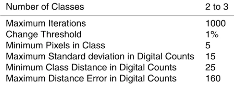
number of classes the data is separated into for clustering within each landcover. Thus, since we assume to know the number of classes, a priori, we have chosen to use the ISODATA technique for the clustering. The statistical thresholds used to separate the classes in the ISODATA analysis are shown in Table 1.

To obtain the data sets for each landcover, masks were created to isolate individual

10

landcover types in the image data using a landcover map. The landcover map used for this study was obtained by analyzing the temporal behavior of vegetation greenness from vegetation indices (NDVI) derived from the same seven images to segregate and identify vegetation with no prior information about the area (DeAlwis et al., 2007). Land cover types were row crop, grass/pasture, shrub, deciduous forest, evergreen forest,

15

and mixed forest (Fig. 1). Using the masks of each of the landcover types, an image cube or stack was then created for the seven DOS corrected NDWI images. The initial NDWI values that varied from –1 to +1 were linearly stretched between zero and 255 by assigning the least NDWI value in each image cube a value of zero and the maximum NDWI a value of 255. The stretch was necessary because the ISODATA clustering

20

algorithm operates only on integer values. The ISODATA technique divided the NDWI values of the image cubes for each land cover type into two or three NDWI regions with significantly different temporal patterns based on the parameter thresholds for clustering shown in Table 1. The pattern in NDWI values for the regions represents the temporal variation of surface soil moisture (before leaf on) and leaf water content

25

(11)

HESSD

4, 1663–1696, 2007

Full Screen / Esc

EGU

2.5 Identification of hydrologically active areas (HAA)

Next we related the NDWI patterns within each land cover to the HAAs in the Town Brook watershed. Town Brook has shallow, highly conductive soils with depths of 30 to 140 cm over a restrictive hardpan. Lateral flow in the shallow surface soil occurs during periods when the precipitation exceeds the potential evaporation and tends to

5

form a saturated area at the bottom of slopes or areas with shallow soils where the storage is exceeded. These HAAs saturate during rainfall events and produce runoff. During the period when potential evapotranspiration exceeds rainfall, the soils dry; in-terflow drains the water from the soil profile and most of the HAAs dry up and can, in fact, dry out more than other soils in the watershed that are deeper and have a greater

10

storage capacity. During the period when precipitation exceeds evapotranspiration we hypothesize that HAA will be detectable on these low storage, shallow soils underlain by a restricting layer. The relatively dry fall and winter period observed in 2000–2001 will further cause the HAAs to be detectable in saturation prone areas when compared to other areas within the same land cover because of the lower storage capacity.

Intu-15

itively, these same areas that saturate during the period when precipitation is greater than evapotranspiration will be drier during the period where evapotranspiration ex-ceeds precipitation (and have lower NDWI values) (Fig. 3). Similarly, regions that had low NDWI during early growing season and high NDWI due to high leaf water content during the growing season are regions with a low propensity to saturate for prolonged

20

periods as indicated by the better vegetative growth conditions (Fig. 3).

2.6 Accuracy assessment

The remotely sensed HAAs were compared with the distributed output of two simula-tion models developed for watersheds such as Town Brook, specifically, the Soil Mois-ture Distribution and Routing (SMDR) model (Frankenberger et al., 1999) and Variable

25

Source Loading Function (VSLF) model (Schneiderman et al., 2007). We also used field measurements of soil moisture levels taken in 2001 (Mehta et al., 2004) and field

(12)

HESSD

4, 1663–1696, 2007

Full Screen / Esc

survey in the upper reaches of the watershed conducted in 2006 to identify frequently saturated areas. Little spatially distributed data on the soil moisture content is readily available, thus, we propose several ways of testing the results: corroboration with ex-isting hydrologic models, direct soil moisture measurements, and field surveys in the watershed. While the simulation model results by no means represent the absolute

5

ground truth we have selected two models that both capture the evolution of HAAs in the landscape, and thus should provide an adequate representation of saturated ar-eas. Models based on topographic indices, such as TOPMODEL (Beven and Kirkby, 1979) with its copious variations and the Soil Moisture Distribution and Routing model (SMDR) (Zollweg et al., 1996; Frankenberger et al., 1999) are two modeling concepts

10

with modest input requirements capable of capturing the spatial distribution of soil mois-ture levels at the watershed scale. Both models have been shown to identify saturated areas, albeit for different types of systems. Topographic index based models generally assume that a watershed wide water table intersects the landscape to produce satu-rated runoff generating areas and SMDR assumes that these areas are controlled by

15

transient inter-flow perched on a shallow restricting layer.

The Soil Moisture Distribution and Routing (SMDR) model is a physically-based, fully-distributed model that simulates the hydrology for watersheds with shallow sloping soils. The model was developed specifically for regions such as Town Brook (Franken-berger et al., 1999). The model combines elevation, soil, and land use data, to predict

20

the spatial distribution of soil moisture, evapotranspiration, saturation-excess overland flow (i.e., surface runoff), and interflow throughout a watershed on a daily time step. Soil moisture content is predicted for each cell, typically of dimension 10 m. SMDR has been extensively validated in Town Brook (Mehta et al., 2004), and other basins in the region (e.g. Frankenberger et al., 1999; Hively et al., 2005; Johnson et al 2004; Easton

25

et al., 2007, more information athttp://soilandwater.bee.cornell.edu/).

The Variable Source Loading Function (VSLF) model (Schneiderman et al., 2007), a derivative of the Generalized Watershed Loading Function (GWLF) model (Haith and Shoemaker, 1987), uses the Soil Conservation Curve Number (SCS-CN) (USDA-SCS,

(13)

HESSD

4, 1663–1696, 2007

Full Screen / Esc

EGU

1972) method to predict runoff. The main difference between the VSLF and GWLF approaches to using the SCS runoff equation is that runoff is explicitly attributable to source areas according to a soil topographic index distribution rather than by land use and soil type as in original GWLF. Runoff and soil moisture are then distributed through-out the watershed according to a spatially weighted soil topographic index (Lyon et al.,

5

2004) VSLF has been used in the Catskill Mountains to predict hydrology and water quality, and has been validated spatially to predict saturated areas (Schneiderman et al., 2007).

The remotely sensed saturated areas were also compared with a field survey (Fig. 6) of saturated areas as well as measured soil moisture content from three transects

10

(Figs. 2 and 7) in Town Brook (Mehta et al., 2004) The field survey was conducted in spring 2006 during the period when HAAs would be most saturated, and should thus compare well with HAAs derived by the NDWI. Figure 2 shows the layout of the three soil moisture sampling transects: T1, T2 and T3. Soil samples from 3–8 cm depth were collected at 10 m intervals along each of the transects (Mehta et al. 2004). The

15

transects covered grass and shrub landcover types. Transect T1 was 210 m long and predominately shrub ending in a grass landcover, sampled on 3 November 2000 after a 15 day dry period following a 1.5 cm rain event. Transect T2, was 230 m long shrub landcover and was sampled on 4 May 2001 after 0.1 cm of rain on the previous day. Transect T3, was 90 m with a grass landcover and was collected on 28 November 2000.

20

3 Results

An average value of NDWI, for each of the seven LANDSAT 7 ETM+ images for the different months was obtained for each of the temporally homogeneous NDWI regions that were identified by the ISODATA clustering method within each of the six landcover types (Table 1). These average NDWI values for the wetness classes are depicted in

25

Fig. 3.

(14)

HESSD

4, 1663–1696, 2007

Full Screen / Esc

landcover types. The NDWI for all landcovers is elevated in January and April when the soil is wet. The lowest NDWI occurred in May after a 15 day dry period reduced the moisture content of the soil surface. The NDWI values increase subsequently for June and July due to the increase in leaf water content. The NDWI values for the deciduous and mixed forest decrease at the end in October (due to leaf senescence).

5

The NDWI for the shrub, evergreen forest, and crop land covers remain stable through the fall, while grass/pasture increase marginally. The slight increase in the NDWI for the grass/pasture is likely due to continued biomass accumulation into the fall, presumably increasing the leaf water content.

Comparing the NDWI curves of deciduous forests, grass, shrub, mixed forests, crop

10

and evergreen forests the landcover types in Fig. 3 it is evident that there is a region among all landcover types that is more wet (high NDWI) in the spring than the other homogeneous regions and drier (low NDWI) late in the growing season. This char-acteristic is consistent among all the landcover types. This region is shown in blue in Fig. 3 and, according to our hypothesis, is identified as the wet region in the

land-15

cover type. Regions within a landcover type having low surface water content during the early growing season and more leaf water content during the late growing season were identified as dry areas that were favorable for plant growth (due to high leaf water content during the late growing season).

Figure 3 shows the greatest variation in NDWI values between March and April 2001,

20

where snow cover went from 20 cm in March to essentially zero in April. The NDWI is high due to the snow cover and the increase in surface soil moisture from snow melt. At the same time the evapotranspiration loss was small and we expected that the HAAs were fully saturated. Thus, during the early growing season the areas with shallow soils, high water table, or a large contributing area tended to saturate and were

25

captured in the NDWI images. During the summer when evapotranspiration exceeds the rainfall and the interflow supplying water from upslope to the HAAs ceases the differences in NDWI values become much less (Fig. 3). During May and June it is reasonable to assume that the increase in the NDWI in most land covers is due to the

(15)

HESSD

4, 1663–1696, 2007

Full Screen / Esc

EGU

increase in the biomass, and subsequent leaf water content from maturing vegetation. During the summer, it is of interest to note that the moisture content in the HAAs that were saturated during the spring snowmelt decreases below that of the remaining land cover types (Fig. 3) because the HAA soils are shallower and thus have less storage.

As a matter of interest, the NDVI values are also calculated for the NDWI wetness

5

classes and show the opposite behavior from that of the NDWI. The NDVI values are low in January and March when there is little biomass and then increase during the rest of the year when plant growth resumes. Detailed information on the differences in NDVI values between land cover types can be found in DeAlwis et al. (2007). What is important here is that the different wetness index classes showed few differences in

10

NDVI values. During January and April when there is little biomass (except for ever-greens), the NDVI values should be the same. During the summer the leaf area index for all land covers is greater than three and thus it is difficult to discriminate among differences in the NDVI signal. The insensitivity to moisture content makes the NDVI signal a good proxy to distinguish land cover types but a poor predictor of moisture

15

status.

3.1 Validation

The main difficulty in comparing the NDWI predicted HAAs is that the remotely sensed saturated areas are static in time and represent an average saturation risk for the year of observation while the saturated areas predicted by SMDR and VSLF are

continu-20

ous, and dynamic in time. That being said, the NDWI saturated areas should represent areas of the landscape most prone to frequent saturation. Thus, to compare the tempo-rally dynamic prediction made by SMDR and VSLF we aggregated predictions during the spring for SMDR and VSLF (March–June 2001), which represents the most prob-able saturated period in this region. The simulated saturation degree maps for SMDR

25

and VSLF were stacked and an average saturation degree was calculated for each of the 10 m×10 m pixels. We resampled the 30 m×30 m NDWI pixels to 10 m×10 m pixel size to compare among models. The area of each specific land cover in Town Brook

(16)

HESSD

4, 1663–1696, 2007

Full Screen / Esc

was calculated and a ratio of total landcover to NDWI saturated area was derived. For example, deciduous forest covers 21 677 pixels of Town Brook, of which 3183 are pre-dicted as saturated by the NDWI, that is, 17.5% of the deciduous forest in Town Brook is predicted as an HAA. Then these areas were extracted independently for each land-cover from the SMDR or VSLF saturation degree maps. We assume that the pixels

5

from the SMDR and VSLF maps with the highest saturation degree corresponding to the fraction of the remotely sensed landcover that was saturated should theoretically correspond with the remotely sensed data (the 17.5% of cells with the highest satura-tion degree for deciduous forest from SMDR and VSLF). This allowed comparison of the potentially saturated areas on an areal basis.

10

The region maps representing the temporally homogeneous NDWI regions for each landcover type were overlaid on the saturation degree map and the mean saturation degree value within each of the regions was calculated. Results of this comparison are shown in Table 2. In all of the landcover types (except evergreen forests) it seems that the common characteristic of the homogeneous regions that are wet (represented by

15

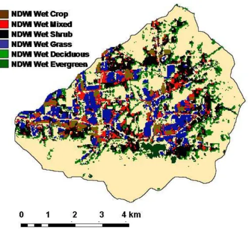
the blue curves in Fig. 3) in the early growing season and dry in the late growing sea-son have higher saturation degrees than those areas predicted as dry. The remotely sensed saturated areas are shown in Fig. 4. The intersection of the NDWI saturated areas and the SMDR and VSLF saturated areas are shown in Fig. 5. The extent of the remotely sensed NDWI based saturated area predictions for the crop, deciduous forest,

20

mixed forest, and shrub were extracted from the GIS and the producer and users ac-curacy were tabulated. Thus we have a measure of where the remotely sensed NDWI saturated areas agree with the SMDR or VSLF saturated areas (producers’ accuracy Table 2). NDWI based predictions not coinciding with an SMDR or VSLF prediction are not shown, but may be abstracted from the user’s accuracy in Table 2. The remotely

25

sensed saturated areas generally agree well with the model predictions with overall accuracies of 0.78 and 0.77 for SMDR and VSLF, respectively. However, saturated areas in the deciduous forest landcover predicted by the remote sensing method do not agree as well with SMDR and VSLF (Table 2). The positions of the NDWI

(17)

satu-HESSD

4, 1663–1696, 2007

Full Screen / Esc

EGU

rated areas within the deciduous forests were accurately predicted but their extent was small compared to the modeled saturated areas. The main discrepancy between the NDWI saturated areas and the modeled saturated areas is likely that the LAI is greater than six in the forest and thus the NDWI becomes saturated and unable to discriminate saturated areas. Additionally, the moisture status of the soil surface likely has limited

5

influence on the water content of the deciduous trees, as they can derive water from deeper in the soil, and thus the leaf water status may be more affected by regional groundwater dynamics then surface phenomena.

Due to the disagreement between the remotely sensed saturated areas and the SMDR and VSLF predicted saturated areas we used field surveying techniques to

10

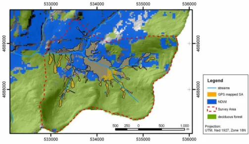
determine the model accuracy. Results from the field mapping survey conducted in an upland portion (deciduous forest) of the Town Brook watershed are shown in Fig. 6. The area was surveyed during spring (most frequently saturated time) 2006 with a GPS unit and saturated areas were mapped (Fig. 6). The mapped extents of the saturated areas generally agree well with the NDWI predicted saturated areas, with an overall

15

accuracy of 75%, better agreement than was calculated for the accuracy between the distributed models (SMDR and VSLF) for the deciduous forest. This provides some evidence that the remotely sensed saturated areas may better capture the true extent of HAAs in forested areas. It should be noted that neither SMDR nor VSLF were intended for application to strictly forested areas and have never really been validated

20

for them, thus the comparison may not be warranted.

Figure 7 shows the distribution of the measured and the simulated soil moisture content along the transects T1–T3. Figure 7 also shows the wet (blue) and dry (red) areas derived from remotely sensed data along the same transects. The simulated soil moisture content showed a good correlation with the measured soil water content.

25

The soil moisture content is seen to decrease in the middle of transact T2 indicating a dry area (Fig. 7b). The remotely sensed data were able to correctly identify a dry area among the wet shrub land along the transact T2. The wet grass and shrub land along transacts T1 (Fig. 7a) and T3 (Fig. 7c) were also correctly identified as wet areas by

(18)

HESSD

4, 1663–1696, 2007

Full Screen / Esc

the remotely sensed NDWI based method. To test the above hypothesis further the SMDR and VSLF predicted saturation degree was compared to the remotely sensed homogeneous regions (Table 3). According to the hypothesis within a landcover type a higher surface water content during the early growing season and lower leaf water content during the late growing season indicates a hydrologically sensitive (saturated)

5

area, that are not favorable for plant growth (represented by the blue curve in Fig. 3).

4 Discussion

In theory, areas within a landcover type situated on a steep slope, deep soils, a high permeability, and a low contributing area should remain drier than those areas with shallow slopes and soils, low permeability, and a large contributing area. In such

steep-10

sloped areas within each landcover type, NDWI is lower during early spring. The depth of the soil, a proxy for soil storage capacity, directly influences the leaf water content in late summer, while the depth of the soil is inversely proportional to the wetness of the soil in early spring.

Analysis of the NDWI data during a complete phenological cycle within a landcover

15

type highlights significant hydrological characteristics within the landcover. While the NDWI varies proportionally with the surface water content before leaf on (early spring) and leaf water content during leaf on (summer), the largest differences were consis-tently detected during the spring (Fig. 3), consistent with the other measurements and model analysis from the region. There were few differences detected during the

sum-20

mer and early fall periods, as watersheds in this region tend to dry out during the period from June to October when evapotranspiration is greater than precipitation. However, there were differences in the NDWI for the crop and pasture land covers during the summer. Specifically, the areas with a higher NDWI in the spring had considerably lower values than other areas in the summer (Fig. 3). There are likely numerous

ex-25

planations for this observation, but several appear more probable. First in these HAAs, the shallow, low storage soils are prone to drying out thus providing inadequate plant

(19)

HESSD

4, 1663–1696, 2007

Full Screen / Esc

EGU

available water to produce similar biomass as the non saturation prone areas. Second, and related to the first, the crop and pasture land covers typically have less developed root systems and probe the soil less aggressively for moisture than the forest or shrub type land covers, making them more susceptible to moisture stress.

The time series of the NDWI images exhibit characteristics consistent with the

hy-5

drologic setting of the landcovers considered. Interestingly evergreen forest behaved differently than the other landcover types. The region that had high NDWI during the early growing season and low NDWI during the late growing season that was hypothe-sized as the wet area (HAA) was predicted as dry according to the hydrological models. The high NDWI measured during the spring was clearly not due to the soil surface

wa-10

ter content as the satellite would not sense the soil surface as the LAI would be well above six. Another reason could be due to the fact that NDWI responds differently to evergreen needles. Further study needs to be done to explain this atypical behavior among the evergreen forests.

A significant issue in using this approach is the availability of the imagery for a

sin-15

gle year. The LANDSAT 7 ETM+ satellite collects imagery over the study area once every 16 days or about 23 times per year. The maximum amount of data that would be available to create a one-year time series would be 23 images. In practice, getting a sequence of six to eight images that are roughly equally-spaced through the year could be difficult with LANDSAT 7 ETM+ data. However, the LANDSAT 7 ETM+ data were

20

selected because its spatial resolution matched the need to identify relatively small re-gions of uniform landcover classes. Where spatial resolution is not so critical, there are satellite-based instruments (e.g. MODIS with 1 km pixels and appropriate spectral bands) that provide coverage every one to two days, and should be capable of provid-ing much more detailed time series. However, the resolution is such that delineatprovid-ing

25

saturated areas can be difficult (only 37 pixels for Town Brook). This invites the ques-tion of how many images are actually required and what the critical time periods are. It is clear that the April image was imperative to capture the saturated areas in the watershed (Fig. 3). It is not clear that both the June and July images were needed

(20)

HESSD

4, 1663–1696, 2007

Full Screen / Esc

as there were only differences detected between classes in the crop and pasture land covers (Fig. 3). These difficulties aside, it appears that the time-series examined here contain unique and useful information, and that the procedure holds significant promise for hydrologic applications.

This series analysis of remotely sensed spectral data has never been used for the

5

identification of HAAs but holds great potential, particularly at large scale since the derivation is independent of field measurements and hydrological parameters. How-ever since this study was conducted in a temperate humid region of the country this method is based specifically on vegetation and likely cannot be used to predict satu-rated areas in semi arid and arid areas, or areas where runoff is genesatu-rated by infiltration

10

excess processes and not from saturated areas of the landscape. The method might successfully be applied to determine relative differences in moisture contents in many areas, VSA or otherwise. Further work is necessary to investigate application of this method to other regions

5 Conclusions

15

Based on the temporal pattern of a wetness index derived from remotely sensed satel-lite imagery we were able to identify HAAs using an unsupervised classification tech-nique. This method is advantageous because it allows identification of HAAs indepen-dent of field measurements at a high spatial resolution. The two images in the early and late growing season contributed substantially to the accuracy of the results and

20

were critical in the sequence, since during these periods plant growth is rapid and re-flective of the stresses to which they are subjugated. The April image collected when there was four cm of snow on the ground, and the May image that was taken after 15 days of drought contributed substantially to the analysis. The largest variation among each homogeneous landcover type was seen on the April image with snow cover. The

25

May image showed the NDWI to decrease due to the 15 precipitation free days prior to the image; the increase in NDWI thereafter was due to increases in the leaf water

(21)

HESSD

4, 1663–1696, 2007

Full Screen / Esc

EGU

content, particularly for the crop and pasture landcovers.

The derived maps of saturated areas were validated by comparison with two dis-tributed hydrologic models; physical data collected in the watershed and mapped sat-urated areas. The results of the validation have shown the remotely sensed data to adequately represent the spatial distribution of saturated areas for most landcovers in

5

the watershed. This technique of delineating saturated areas shows promise for many applications requiring knowledge of HAAs, such as hydrologic modeling, landuse plan-ning, zoplan-ning, or implementing management practices to reduce pollution.

References

Bernier, P. Y.: Variable source areas and stormflow generation, An update of the concept and 10

a simulation affect, Soil Sci. Soc. Am. J., 79, 195–213, 1985.

Beven, K. J. and Kirkby, M. J.: A physically-based, variable contributing area model of basin hydrology, Hydrol. Sci. Bull., 24, 43–69, 1979.

Beven, K. J.: Changing ideas in hydrology, the case of physically based models, J. Hydrol., 105, 157–172, 1989.

15

Beven, K. J.: Rainfall-runoff modeling: the primer, John Wiley & Sons, LTD. Chichester, Eng-land. 360pp, 2001.

Bindlish, R., Jackson, T. J., Wood, E., Huilin, G., Starks, P., Bosch, D., and Lakshmi, V.: Soil moisture estimates from TRMM Microwave Imager observations over the Southern United States, Remote Sens. Environ., 85, 507–515, 2003.

20

Bowman, R. A.: A sequential extraction procedure with concentrated sulfuric acid and a dilute base for soil organic phosphorus, Soil Sci. Soc. Am. J., 53, 362–366, 1989.

Ceccato, P., Flasse, S., Tarantola, S., Jacquemoudy, S., and Gr’egoire, J. M.: Detecting vege-tation leaf water content using reflectance in the optical domain, Remote Sens. Environ., 77, 22–33, 2001.

25

Chavez, P. S.: An improved dark-object subtraction technique for atmospheric scattering cor-rection of multispectral data, Remote Sens. Environ., 24(3), 459–479, 1988.

Chen, J. M. and Cihlar, J.: Retrieving leaf area index of boreal conifer forests using LANDSAT TM images, Remote Sens. Environ., 55, 153–162, 1996.

(22)

HESSD

4, 1663–1696, 2007

Full Screen / Esc

Interactive Discussion Cohen, W. B., Maiersperger, T. K., Gower, S. T., and Turner, D. P.: An improved strategy for

regression of biophysical variables and LANDSAT ETM+data, Remote Sens. Environ., 84, 561–571, 2003.

DeAlwis, D.A.: Identification of hydrologically active areas in the landscape using satellite im-agery, Dissertation, Cornell University, Ithaca, NY USA, 2007.

5

De Jong, R., Shields, J. A., and Sly, W. K.: Estimated soil water reserves applicable to a wheat-fallow rotation for generalized soil areas mapped in southern Saskatchewan, Canadian J. Soil Sci., 64(3), 667–680, 1984.

Delbart N., Le Toan , T., Kergoat, L., and Fedotova, V.: Remote Sensing of spring phenology in boreal regions: A free of snow-effect method using NOAA-AVHRR and SPOT-VGT data 10

(1982–2004), Remote Sens. Environ., 101(1), 52–62, 2006.

Dunne, T. and Leopold, L: Water in Environmental Planning, W. H. Freeman & Co., New York. 818pp, 1978.

Dunne, T. and Black, R. D.: Partial area contributions to storm runoff in a small New England watershed, Water Resour. Res., 6, 1296–1311, 1970.

15

Easton, Z. M., G ´erard-Marchant, P., Walter, M. T., Petrovic, A. M., and Steenhuis, T. S.: Hy-drologic assessment of a urban variable source watershed in the northeast United States, Water Resour. Res., 43 W03413, doi:10.1029/2006WR005076, 2007.

Fassnacht, K. S., Gower, S. T., MacKenzie, M. D., Nordheim, E. V., and Lillesand, T. M.: Esti-mating the leaf area index of north central Wisconsin forests using the LANDSAT Thematic 20

Mapper, Remote Sens. Environ., 61, 229–245, 1997.

Farrar, T. J., Nicholson, S. E., and Lare, A. R.: The influence of soil type on the relationships between NDVI, rainfall, and soil moisture in semiarid Botswana, Remote Sens. Environ., 50(2), 121–133, 1994.

Fensholt, R.: Earth observation of vegetation status in the Sahelian and Sudanian West Africa, 25

comparison of Terra MODIS and NOAA AVHRR satellite data, Int. J. Remote Sens., 25(9), 1641–1659, 2004.

Frankenberger, J. R., Brooks, E. S., Walter, M. T., Walter, M. F., and Steenhuis, T. S.: A GIS based variable source area hydrology model, Hydrol. Proc., 13, 805–822, 1999.

Friedl, M. A., Michaelsen, J., Davis, F. W., Walker, H., and Schimel, D. S.: Estimating grassland 30

biomass and leaf area index using ground and satellite data, Int. J. Remote Sens., 15, 1401– 1420, 1994.

(23)

HESSD

4, 1663–1696, 2007

Full Screen / Esc

EGU

Opt., 4, 11–20, 1965.

Gao, B.: NDWI. A normalized difference water index for remote sensing of vegetation liquid water from space, Remote Sens. Environ., 58(3), 257–266, 1996.

Grayson, R. B., Moore, I. D., and McMahon, T. A.: Physically based hydrologic modeling, 1, A terrain-based model for investigative purposes, Water Resour. Res., 28, 2639–2658, 1992. 5

Guha, A. and Lakshmi, L.: Sensitivity, spatial heterogeneity, and scaling of C-Band microwave brightness temperatures for land hydrology studies, IEEE Trans. Geosci. Remote Sensing, 40(12), 2626–2635, 2002.

Haith, D. A. and Shoemaker, L. L.: Generalized Watershed Loading Functions for stream flow nutrients, Water Resour. Bull., 23(3), 471–478, 1987.

10

Hively, W. D., Gerard-Marchant P., and Steenhuis, T. S.: Distributed hydrological modeling of total dissolved phosphorus transport in an agricultural landscape, part II, dissolved phospho-rus transport, Hydrol. Earth Syst. Sci., 10, 263–276, 2006,

http://www.hydrol-earth-syst-sci.net/10/263/2006/.

Hunt Jr., E. R., Rock, B. N., and Nobel, P. S.: Measurement of leaf relative water content by 15

infrared reflectance, Remote Sens. Environ., 22, 429–435, 1987.

Karnieli, A., Kaufman, Y., Remer, L., and Wald, A.: AFRI – aerosol free vegetation index, Remote Sens. Environ., 77(1), 10–21, 2001.

Kerr, Y. H.: Soil moisture from space: Where are we? Hydrogeol. J., 15, 117–120, 2007. Killelea, M.: Carbon storage in New York State forestland, Ph.D. Dissertation, Cornell Univer-20

sity, Ithaca, NY, USA, 2005.

Law, B. E. and Waring, R. H.: Remote sensing of leaf area index and radiation intercepted by understory vegetation, Ecol. Apps., 4, 272–279, 1994.

Lyon, S. W., Walter, M. T., Gerard-Marchant, P., and Steenhuis, T. S.: Using a topographic index to distribute variable source area runoff predicted with the SCS curve-number equation, 25

Hydrol. Proc., 18, 2757–2771, 2004.

Mehta, V. K., Walter, M. T., Brooks, E. S., Steenhuis, T. S., Walter, M. F., Johnson, M., Boll, J., and Thongs, D.: Application of SMR to modeling watersheds in the Catskill Mountains. Environ, Model. Assess., 9, 77–89, 2004.

National Oceanic and Atmospheric Administration (National Climatic Data Center), Weather 30

data [Online], Available byhttp://www.ncdc.noaa.gov/oa/ncdc.html, 2001.

Needelman, B. A., Gburek, W. J., Petersen, G. W., Sharpley, A. N., and Kleinman, P. J. A.: Surface runoff along two agricultural hillslopes with contrasting soils, Soil Sci. Soc. Am. J.,

(24)

HESSD

4, 1663–1696, 2007

Full Screen / Esc

Interactive Discussion 68, 914–923, 2004.

Nicholson, S. E. and Farrar T. J.: The influence of soil type on the relationships between NDVI, rainfall, and soil moisture in semiarid Botswana, Remote Sens. Environ., 50, 107–120, 1994. New York City Department of Environmental Protection (NYCDEP), Modeling Status Report –

FAD 303b-1, 2004. 5

Research Systems, Inc. ENVI Users Manual, What’s new in ENVI 4.0 ENVI Version 4 Edi-tion, Boulder, Colorado, 2002.

Richardson, A. J., Wiegand, C. L., Wanjura, D. F., Dusek, D., and Steiner, J. L.: Multisite analyses of spectral-biophysical data for Sorghum, Remote Sens. Environ., 41(1), 71–82, 1992.

10

Schmugge, T.: Remote sensing of soil moisture, in: Hydrological Forecasting, edited by: An-derson, M. G. and Burt, T. P., Wiley, New York, 101–124, 1985.

Schneiderman, E. M., Pierson, D. C., Lounsbury, D. G., and Zion, M. S.: Modeling the hy-drochemistry of the Cannonsville watershed with Generalized Watershed Loading Functions (GWLF), J. Am. Water Resour. Assoc., 38(5), 1323–1347, 2002.

15

Schneiderman, E. M., Steenhuis, T. S., Thongs, D. J., Easton, Z. M., Zion, M. S., Mendoza, G. F., Walter, M. T., and Neal, A. L.: Incorporating variable source area hydrology into the curve number based Generalized Watershed Loading Function model, Hydrol. Proc., in press, 2007.

Timlin, D. J., Pachepsky, Y., Walthall, C. L., and Loechel, S. E.: The use of a water-budget 20

model and yield maps to characterize water availability in a landscape, Soil and Tillage, 58, 219–231, 2001.

Tucker, C. J.: Remote sensing of leaf water content in the near infrared, Remote Sens Environ., 10, 23–32, 1980.

USDA-SCS (Soil Conservation Service): National Engineering Handbook, Part 630 Hydrology, 25

Section 4, Chapter 10, 1972.

Wagner, W., Naeimi V., Scipal K., de Jeu R., and Martinez-Fernandez J.: Soil moisture from operational meteorological satellites, Hydrogeology J. 15, 121–131, 2007.

Wang, J., Price, K. P., and Rich, P. M.: Spatial patterns of NDVI in response to precipitation and temperature in the central Great Plains, Int. J. Remote Sens., 22(18), 3827–3844, 2001. 30

Wang, J. R. and Schmugge, T. J.: An empirical model for the complex dielectric permittivity of soils as a function of water content, IEEE Trans. Geosci. Remote Sens., 18(4), 288– 295, 1980.

(25)

HESSD

4, 1663–1696, 2007

Full Screen / Esc

EGU

Whiting, M. L., Lin, L., and Ustin S. L.: Predicting water content using Gaussian model on soil spectra, Remote Sens. Environ., 89(4), 535–552, 2004.

Wigmosta, M. S., Vail, L. W., and Lettenmaier, D. P.: A distributed hydrology vegetation model for complex terrain, Water Resour. Res., 30, 1665–1679, 1994.

Xiao, X., Boles, S., Liu, J. Y., Zhuang, D. F., and Liu, M. L.: Characterization of forest types in 5

Northeastern China, using multi-temporal SPOT-4 VEGETATION sensor data, Remote Sens. Environ., 82, 335–348, 2002.

Yang, J. P., Ding, Y. J., and Chen, R. S.: Spatial and temporal of variations of alpine vegetation cover in the source regions of the Yangtze and Yellow Rivers of the Tibetan Plateau from 1982 to 2001, Environ. Geo., 50(3), 313–322, 2006.

10

Zollweg, J. A., Gburek, W. J., and Steenhuis, T. S.: SMoRModA GIS-integrated rainfall-runoff model applied to a small northeast U.S. watershed, Trans. ASAE, 39, 1299–1307, 1996.

(26)

HESSD

4, 1663–1696, 2007

Full Screen / Esc

Table 1. Parameter set used in the ISODATA analysis.

Number of Classes 2 to 3 Maximum Iterations 1000

Change Threshold 1%

Minimum Pixels in Class 5 Maximum Standard deviation in Digital Counts 15 Minimum Class Distance in Digital Counts 25 Maximum Distance Error in Digital Counts 160

(27)

HESSD

4, 1663–1696, 2007

Full Screen / Esc

EGU Table 2. Producers (PA) and Users Accuracy (UA) assessment of remotely sensed saturated

areas compared to the equivalent areal extent by landcover of saturated areas predicted using the Soil Moisture Distribution and Routing (SMDR) model and the Variable Source Loading Function (VSLF) model. The SMDR and VSLF areas are considered ground truth for the clas-sification comparison.

Landcover SMDR wet NDWI wet Overlap PA UA Deciduous forest 1111 3783 834 0.75 0.22 Grass 5150 4170 3626 0.70 0.87 Shrub 7196 6139 5758 0.80 0.94 Mixed forest 2796 2378 2349 0.84 0.99 Row crop 1378 1255 1240 0.90 0.99 Total 17631 17725 13807 Overall Accuracy 0.78

VSLF wet NDWI wet Overlap PA UA Deciduous forest 1723 3783 1522 0.88 0.40 Grass 3889 4170 2632 0.68 0.63 Shrub 7320 6139 5883 0.80 0.96 Mixed forest 2776 2378 2337 0.84 0.98 Row crop 1365 1255 1244 0.91 0.99 Total 17073 17725 13618 Overall Accuracy 0.77

(28)

HESSD

4, 1663–1696, 2007

Full Screen / Esc

Table 3. Mean saturation degree for the Soil Moisture Distribution and Routing model (SMDR)

and the Variable Source Loading Function model (VSLF) for the Normalized Difference in Wa-ter Index (NDWI) homogeneous regions in each of the vegetation types. The Region Colors represent the colors used to plot the temporal behavior of the respective regions in Fig. 3. The region color blue represents Normalized Difference in Water Index (NDWI) predicted as saturated (wet) areas for each of the landcover types.

Landcover Region Color SMDR Saturation Degree VSLF Saturation Degree cm3H₂O cm−3_soil

Deciduous Forest Blue 0.70 0.68

Green 0.59 0.56 Red 0.51 0.34 Grass/Pasture Blue 0.65 0.71 Cyan 0.56 0.53 Red 0.36 0.47 Shrub Blue 0.57 0.65 Red 0.34 0.36

Mixed Forest Blue 0.62 0.67

Red 0.39 0.39

Crop Blue 0.60 0.69

Red 0.45 0.41

Evergreen Forest Blue 0.28 0.51

(29)

HESSD

4, 1663–1696, 2007

Full Screen / Esc

EGU Fig. 1. Landcover in the Town Brook watershed (DeAlwis et al., 2007). Inset figure gives the

(30)

HESSD

4, 1663–1696, 2007

Full Screen / Esc

Fig. 2. Landscape soil moisture sampling transects (Mehta et al., 2004) overlaid on a digital

elevation model of Town Brook. Soil moisture samples were taken along the T1, T2 and T3 transacts.

(31)

HESSD

4, 1663–1696, 2007

Full Screen / Esc

EGU Fig. 3. Variation of the Normalized Difference in Water Index (NDWI) of the two to three

homo-geneous regions in each of the landcover types (as defined by ISODATA analysis for (a) Row Crop, (b) Deciduous Forests (c) Evergreen Forests (d) Grass/Pasture, (e) Mixed Forests, (f) Shrub. Blue lines in all figures show the NDWI for predicted saturated zones, red lines show the NDWI for predicted unsaturated zones, in grass/pasture and deciduous forest the light blue and green lines show the NDWI for zones of intermediate saturation.

(32)

HESSD

4, 1663–1696, 2007

Full Screen / Esc

Fig. 4. Normalized Difference in Water Index (NDWI) predicted saturated (wet) areas for each

(33)

HESSD

4, 1663–1696, 2007

Full Screen / Esc

EGU Fig. 5. (a) Saturated areas by landcover predicted by the Variable Source Loading Function

(VSLF) model: (b) Intersection of saturated areas predicted by the NDWI and those predicted by VSLF: (c) saturated areas by landcover predicted by the Soil Moisture Distribution and Rout-ing (SMDR) model: (d) Intersection of saturated areas predicted by the NDWI and those pre-dicted by SMDR.

(34)

HESSD

4, 1663–1696, 2007

Full Screen / Esc

Fig. 6. Field survey delineated saturated areas in a portion of the Town Brook watershed

(35)

HESSD

4, 1663–1696, 2007

Full Screen / Esc

EGU Fig. 7. Simulated and measured soil moisture along transects with associated remotely sensed

wet and dry areas (Mehta et al., 2004). Simulated results are from the Soil Moisture Distribution and Routing (SMDR) model.