HAL Id: hal-00230322
https://hal.archives-ouvertes.fr/hal-00230322
Submitted on 10 Feb 2020
HAL is a multi-disciplinary open access
archive for the deposit and dissemination of sci-entific research documents, whether they are pub-lished or not. The documents may come from teaching and research institutions in France or abroad, or from public or private research centers.
L’archive ouverte pluridisciplinaire HAL, est destinée au dépôt et à la diffusion de documents scientifiques de niveau recherche, publiés ou non, émanant des établissements d’enseignement et de recherche français ou étrangers, des laboratoires publics ou privés.
A correction method for turbulence measurements with
a 3D acoustic Doppler velocity profiler
David Hurther, Ulrich Lemmin
To cite this version:
David Hurther, Ulrich Lemmin. A correction method for turbulence measurements with a 3D acoustic Doppler velocity profiler. Journal of Atmospheric and Oceanic Technology, American Meteorological Society, 2001, 18 (3), pp.446-458. �10.1175/1520-0426(2001)0182.0.CO;2�. �hal-00230322�
A Correction Method for Turbulence Measurements with a 3D Acoustic
Doppler Velocity Profiler
D. HURTHER AND U. LEMMIN
Laboratoire de Recherches Hydrauliques, E´ cole Polytechnique Fe´de´rale de Lausanne, Lausanne, Switzerland
ABSTRACT
A method is proposed to reduce the noise contribution to mean turbulence parameters obtained by 3D acoustic Doppler velocity profiler measurements. It is based on a noise spectrum reconstruction from cross-spectra evaluations of two independent and simultaneous measurements of the same vertical velocity component over the whole water depth. The noise spectra and the noise variances are calculated and removed for the three fluctuating velocity components measured in turbulent, open-channel flow. The corrected turbulence spectra show a25/3 slope over the whole inertial subrange delimited by the frequency band of the device, while the uncorrected turbulence spectra have flat high-frequency regions typical for noise effects. This method does not require any hypothesis on the flow characteristics nor does it depend on device-dependent parameters. The corrected profiles of turbulence intensities, turbulent kinetic energy, shear stress, and turbulent energy balance equation terms, such as production, transport, and dissipation, are in better agreement with different semitheo-retical formulas and other measurements from the literature than those from the uncorrected data. Combined with the use of a phase array emitter, the proposed correction method allows measurements with a relative error under 10% in the outer flow region. The corrected inner flow region measurements are still affected by errors that may originate from spatial averaging effects within the sample volume due to the high local velocity gradient or the lack of validity of the universal laws concerning turbulence quantities over a rough bed.
1. Introduction
Over the past decades, high-resolution multistatic ul-trasonic velocity profilers working with coherent de-modulation of the backscattered Doppler phase have been of increasing interest in the fields of fluid dynam-ics, physical oceanography, and, more recently, sedi-ment transport and river hydrodynamics. They have shown their advantage particularly in field applications where the presence of particulate matter often does not allow measurements by other techniques.
In all turbulent flows the precision and the identifi-cation of noise sources are of great importance. In this respect, the mean flow can be treated separately from the turbulent component. When classical hydraulic mean flow characteristics are estimated from high-res-olution sonar data, the precision of the measurements is typically better than 4% (Rolland 1994; Lemmin and Rolland 1997) confirming their high reliability. The re-maining error is mainly due to the precision of posi-tioning the sensors.
Noise effects are of particular importance if turbulence
Corresponding author address: Ulrich Lemmin, LRH-DGC, E´ cole Polytechnique Fe´de´rale de Lausanne, CH-1015 Lausanne, Switzer-land.
E-mail: [email protected]
measurements are evaluated because they are directly based on the fluctuating quasi-instantaneous velocity field estimation. In that case several mechanisms inherent to the measurement technique may reduce the precision. Several authors, Garbini et al. (1982), Lhermitte and Lemmin (1994), Voulgaris and Trowbridge (1998), have worked on the theoretical and experimental identification of the noise sources affecting the turbulence measure-ments with ultrasonic Doppler velocity profilers.
These undesired physical processes can be classified as follows: 1) the Doppler ambiguity process that is char-acterized by the amplitude modulation of the backscat-tered signal related to the transit time of the acoustical targets through the measurement volume. 2) The spatial averaging of the instantaneous velocity field (a large number of targets are present instantaneously), which is taken over the sample volume weighted by the directivity function of the emitter. 3) The effect of the mean flow shear stress present within the sample volume. 4) The phase distortion effect of the emitted front wave. 5) The effect of those turbulent scales that are of the same order of magnitude or smaller than the sample volume’s trans-verse size. 6) The electronic circuitry’s sampling errors linked to the A/D conversion. Except for the spatial av-eraging process (process 2), all other noise sources enter as additional variance terms in the measured fluctuating velocities variances and therefore are statistically
inde-pendent. Due to the geometrical configuration of the sen-sors these noise variances have different values depen-dent on which component (longitudinal, vertical, or trans-verse) is measured. This relates to different weighting factors for the total noise variance common to all com-ponents, as will be shown later.
Correction methods for the mean turbulence mea-surements expressed as additional variances broadly fall into two different categories, described in the next two subsections.
a. Indirect correction method
This method is most frequently used (Lhermitte and Lemmin 1994; Zedel et al. 1996). The different noise variance terms are estimated as a function of the sample volume’s distance from the sensors (processes 1, 3, 4, 5 above). They are added together to form the total noise variance, and a factor is applied to each component to remove the corresponding term from the measured var-iance. Three main disadvantages can be identified:
R The evaluation of the different noise variances is
based on assumptions about specific flow conditions. Variance 3 is calculated by assuming the logarithmic distribution of the mean longitudinal velocity profile. Variance 5 requires the knowledge of the turbulence dissipation rate (Cabrera et al. 1987), computed from expressions valid for isotropic turbulence.
R The transverse size of the sample volume has to be
known (Voulgaris and Trowbridge 1998) to calculate variances 1, 4, and 5. It can either be estimated from acoustical beam approximations or be measured di-rectly (Lhermitte and Lemmin 1994). The noise term related to process 6 also has to be evaluated from additional measurements (Zedel et al. 1996) because an expression for the phase resolution uncertainty can-not be established.
R No direct correction of the turbulence power spectral
density is possible even if the noise variances are evaluated correctly.
b. Correction method based on two point cross correlation
This method, proposed by Garbini et al. (1982) as-sumes that the noise signals (variances 1, 3, 4, and 5) between two points in the velocity profile are uncorre-lated. It should be noted that Garbini et al. (1982) used a monostatic acoustic Doppler velocity profiler (ADVP), where one transducer serves as emitter and receiver. In that case the cross correlation has to be applied to two spatially separated volumes in the velocity profile to en-sure that the noise processes are uncorrelated.
The advantage is that it can directly be applied to measured data and does not require any prediction as does the indirect correction method. The disadvantage is that the target population in the two sample volumes,
to which the cross correlation is applied, has to be dif-ferent to ensure the decorrelation. The existence of over-lapping regions between two consecutive volumes in the profiles, which have to be inclined with respect to the flow direction, limits the decorrelation of the noise part. The method is applied to two volumes separated by one measuring volume, which decreases the noise but in turn also attenuates the desired velocity signal. Our experience has shown that this method cannot be used with multistatic Doppler systems.
In the present paper, a correction method is presented to reduce the effects of variances 1, 3, 4, 5, and 6. The main contribution to noise reduction presented here con-cerns a direct treatment of the data similar the one pro-posed by Garbini et al. (1982). The essential difference is that it can be used with a multistatic 3D-ADVP sensor configuration. We will discuss the efficiency of the method as a function of the flow depth in boundary layer appli-cations such as open-channel flow where the improvement can be compared against the exsisting universal laws.
2. Description of the 3D-ADVP
a. General principle
The 3D-ADVP is composed of the 1-MHz focused phase array emitter (TRA), discussed in Hurther and Lemmin (1998), which is installed vertically in the cen-ter. This is an ultrasonic constant beamwidth transducer system, which is capable of generating an extended focal zone by electronically focusing the beam over the de-sired water depth range. The sample volume has a con-stant width (;7 mm from 26 dB acoustic beam mea-surements) over a range of 60 cm. Due to this config-uration, the effects of process 2 and variance 4 cited in the introduction can be significantly reduced.
Four 1-MHz large angle receivers are placed sym-metrically around the emitter (Fig. 1a). They are used to obtain the velocity components in the tilted direc-tions, TRB, TRC, TRD, and TRE. For the data analysis, the system is divided into two independently working multistatic subsystems (each multistatic system is com-posed of two bistatic configurations). The first subsytem is oriented in the longitudinal plane (TRA, TRB, TRC) of the flow, and measures the vertical and longitudinal instantaneous velocity profiles over the whole water depth. The second one is oriented in the transverse di-rection (TRA, TRD, TRE) of the flow, and allows the vertical and transverse instantaneous velocity profiles to be measured simultaneously with the longitudinal plane. Five sinusoidal sound pulses of identical duration are emitted by the elements of the focused transducer at a fixed pulse repetition frequency (PRF). PRF is chosen to cover the investigated water column and also to ensure a high temporal resolution. Between two pulses, TRB, TRC, TRD, and TRE receive the sound scattered from the same volume in the beam generated by TRA. All signals are simultaneously digitized and gated into M consecutive
FIG. 1. (a) 3D acoustic Doppler velocity profiler configuration for open-channel flow application. TRA represents the phase array emitter, TRB, TRC, TRD, and TRE are the four large angle receivers arranged to compose two independently, simultaneously measuring tristatic subsystems in the longitudinal and transverse flow sections. (b) Schematic diagram showing the longitudinal subsystem and its velocity vector decomposition. (c) Velocity vector decomposition for the transverse subsystem.
sample volumes to provide, after processing, two quasi-instantaneous local velocity profiles in the two planes and over the whole insonified water depth.
The 3D velocity vector components are shown in Figs. 1b and 1c. The Doppler frequency corresponding to each sample volume Rj(j5 1, . . . , M) is calculated
using the pulse-pair algorithm (Lemmin and Rolland 1997). For each of the two multistatic subsystems, the two local Doppler frequencies ( fd1,jand fd2,jfor the
lon-gitudinal system, fd3,jand fd4,jfor the transverse system)
are: 2 f0 2 f0 fd1, j 5 cos(a /2)V1, j 1, j fd3, j5 cos(a /2)V3, j 3, j c c 2 f0 2 f0 fd2, j5 cos(a /2)V2, j 2, j fd4, j5 cos(a /2)V4, j 4, j c c (1) where Vi,jare the projections of the local instantaneous
velocity Vjon the Bragg wavenumber vectors KBi,jwith
i 5 1, . . . , 4 and j 5 1, . . . , M. From these Doppler
frequencies we can determine the longitudinal, trans-verse, and two vertical components of the quasi-instan-taneous velocity vector over the whole insonified water column as c uj5 [ fd1, j2 f ]d2, j 2 f sin0 a1, j c y 5j [ fd3, j2 f ]d4, j 2 f sin0 a3, j c wj,t5 [ fd3, j1 f ]d4, j 2 f (10 1 cosa )3, j c wj,l5 [ fd1, j 1 f ],d2, j (2) 2 f (10 1 cosa )1, j
where subscript l denotes the longitudinal tristatic
sub-system and t the transverse one. Here f0is the emitted
sound wave frequency and c the speed of sound for our water condition. It is noted that two independent esti-mates of the vertical velocity are obtained simulta-neously with this system.
The temporal resolution is fixed by PRF and by the number Npp of consecutive samples needed to estimate
a quasi-instantaneous velocity by the pulse-pair algo-rithm. The corresponding Nyquist frequency is PRF/ (2Npp) [in our case equal to 666.67/(2 3 16) ù 20.84
Hz].
b. Expression of mean turbulence characteristics in terms of geometrical configuration and noise
The measured mean turbulent characteristics that can be expressed as a function of the bistatic configuration (subscript i) and as a function of the measurement po-sition (subscript j) can be written as the sum of the true quantity and the noise contribution. The measured fluc-tuations of the radial velocities can be composed as
^ &(t) 5 ^ &(t) 1 ^nV9i,j V˜9i,j i,j&(t). (3)
All terms are quasi-instantaneous quantities. The fluc-tuating quantities are noted by a prime. Here^ & indicates spatial averaging weighted by the transducer’s directiv-ity function. The tilde denotes the true flow quantities. The term ni,j(t) is the instantaneous noise signal for
com-ponent i at location j.
As suggested by Lohrmann et al. (1995), the follow-ing assumptions are made concernfollow-ing the noise signal:
R the noise signal has a flat power spectral density over
the investigated frequency band PRF/(2Npp) (white
noise)
R it is unbiased
R it is statistically independent of the velocity
TABLE1. Constants depending on the geometrical configuration. The first three columns are the normalized water depth, the distance from the emitter (TRA, see Fig. 1a), and the Doppler angle, respec-tively. The last three columns are the noise weighting factors for the vertical, horizontal turbulence variances, and the turbulence kinetic energy, respectively. z/h dj(cm) aj(8) aj bj aj1 bj/2 0.97 0.94 0.90 0.87 0.84 0.81 0.78 0.75 0.71 22.9300 23.2550 23.5850 23.9100 24.2300 24.5550 24.8800 25.2050 25.5300 24.4172 24.1324 23.8543 23.5827 23.3175 23.0540 22.8008 22.5491 22.3072 11.1806 11.4421 11.7065 11.9737 12.2437 12.5213 12.7972 13.0806 13.3622 0.5234 0.5228 0.5223 0.5218 0.5213 0.5208 0.5203 0.5199 0.5194 11.4423 11.7035 11.9676 12.2346 12.5044 12.7817 13.0573 13.3405 13.6219 0.68 0.65 0.62 0.59 0.56 0.53 0.50 0.46 0.43 0.40 25.8500 26.1750 26.4950 26.8200 27.1400 27.4600 27.7850 28.1050 28.4250 28.7450 22.3072 22.0665 21.8312 21.6047 21.3793 21.1587 20.9426 20.7311 20.5239 20.3209 13.3622 13.6515 13.9438 14.2341 14.5323 14.8334 15.1375 15.4445 15.7545 16.0675 0.5194 0.5190 0.5186 0.5182 0.5178 0.5174 0.5171 0.5167 0.5164 0.5161 13.6219 13.9110 14.2031 14.4932 14.7912 15.0921 15.3960 15.7029 16.0127 16.3255 0.37 0.34 0.31 0.28 0.25 0.22 0.18 0.15 0.12 0.09 0.06 0.03 29.0650 29.3850 29.7050 30.0250 30.3450 30.6650 30.9850 31.3050 31.6250 31.9400 32.2600 32.5800 20.1219 19.9269 19.7357 19.5483 19.3644 19.1840 19.0041 18.8305 18.6601 18.4901 18.3258 18.1646 16.3834 16.7024 17.0242 17.3491 17.6769 18.0076 18.3470 18.6837 19.0234 19.3719 19.7176 20.0662 0.5157 0.5154 0.5151 0.5148 0.5146 0.5143 0.5140 0.5137 0.5135 0.5132 0.5130 0.5128 16.6413 16.9601 17.2818 17.6065 17.9341 18.2648 18.6040 18.9406 19.2802 19.6285 19.9741 20.3226
R it is uncorrelated between the different radial
com-ponents i.
The validity of these assumptions will be demonstrat-ed as part of the verification of the method.
1) VARIANCES
The variance of the radial velocity components is given by
2 ˜ 2 2
^V9 & 5 ^V9 & 1 ^s &,i, j i, j i, j (4) where the second term of the right member of Eq. (4) is the variance of the noise signal. The velocity vari-ances can then be written as
1
2 2 2
^u9 & 5j 2 (^V9 & 1 ^V9 & 2 2^V9 &^V9 &)1, j 2, j 1, j 2, j
4 sin (a /2)j
1
2 2
5 ^u˜9 & 1j 2 ^s &j
2 sin (a /2)j
1
2 2 2
^y9 & 5j 2 (^V9 & 1 ^V9 & 2 2^V9 &^V9 &)3, j 4, j 3, j 4, j
4 sin (a /2)j
1
2 2
5 ^y˜9 & 1j 2 ^s &j
2 sin (a /2)j
1
2 2 2
^w9 & 5j,l 2 (^V9 & 1 ^V9 & 2 2^V9 &^V9 &)1, j 2, j 1, j 2, j
4 cos (a /2)j 1 2 2 5 ^w˜9 & 1j 2 ^s &j 2 cos (a /2)j to obtain 2 2 2 2 2 2
^u9 & 5 ^u˜9 & 1 a ^s &j j j j ^y9 & 5 ^y˜9 & 1 a ^s &j j j j
2 2 2
^w9 & 5 ^w˜9 & 1 b ^s &,j,l j j j (5) assuming that a1,j 5 a2,j 5 a3,j5 a4,j5 ajand ^ & 2
si,j
5 ^ &. This implies that the receiver transducers ares2 j
identical and ideal. This hypothesis will be verified in section 5a. The coefficients ajand bjare related to the
geometrical configuration of the 3D-ADVP (Fig. 1; Ta-ble 1).
In Table 1, the variables djand ajrepresent the
dis-tances of the measurement point j from the emitter and the Doppler angle at measurement point j, respectively. The horizontal velocity components are much more af-fected by noise (due to the geometrical configuration) than the vertical component. Furthermore, the weighting factors for the vertical component are nearly indepen-dent of location j, while the factors affecting the vari-ances of the horizontal components change strongly.
2) KINETIC ENERGY
The kinetic energy can be expressed as
2
˜
^K & 5 ^K & 1 (a 1 b /2)^s & withj j j j j
1 2 2 2
^K & 5 (^u9 & 1 ^y9 & 1 ^w9 &).j j j j,l (6) 2
3) REYNOLDS STRESS TERMS AND TRICOVARIANCES
With the same approach as outlined above, we obtain the Reynolds stress and tricovariance terms entering in the turbulent energy balance equation for a 2D mean flow:
1 ˜ 2 ˜ 2
^u9w9 & 5j j,l (^V9 & 2 ^V9 &) 5 ^u9w9 &,1, j 2, j j j,l (7) 2 sin(a )j
1
3 ˜ 3 ˜ 3 ˜ 2 ˜
^u9 & 5j 3 (^V9 & 2 V9 & 1 3^V9 &^V9 &1, j 2, j 1, j 2, j
8 sin (a /2)j
2 3
˜ ˜
2 3^V9 &^V9 &) 5 ^u9 &2, j 1, j j
1
3 ˜ 3 ˜ 3 ˜ 2 ˜
^y9 & 5j 3 (^V9 & 2 ^V9 & 1 3^V9 &^V9 &3, j 4, j 3, j 4, j
8 sin (a /2)j
2 3
˜ ˜
2 3^V9 &^V9 &) 5 ^y9 &3, j 4, j j
1
3 ˜ 3 ˜ 3 ˜ 2 ˜
^w9 & 5j,l 3 (^V9 & 2 ^V9 & 1 3^V9 &^V9 &1, j 2, j 1, j 2, j
8 cos (a /2)j
2 3
˜ ˜
1 2 ^u9 w9 & 5j j,l 4 sin(a ) sin(a /2)j j 3 3 2 2 ˜ ˜ ˜ ˜ ˜ ˜
3 (^V9 & 1 ^V9 & 2 ^V9 &^V9 & 2 ^V9 &^V9 &)1, j 2, j 1, j 2, j 1, j 2, j 2 5 ^u˜9 w˜9 &j j,l 1 2 ^y9 w9 & 5j j,t 4 sin(a ) sin(a /2)j j 3 3 2 2 ˜ ˜ ˜ ˜ ˜ ˜
3 (^V9 & 1 ^V9 & 2 ^V9 &^V9 & 2 ^V9 &^V9 &)3, j 4, j 3, j 4, j 3, j 4, j 2
5 ^y˜9 w˜9 &.j j,t (9)
There are no contributions from noise signals to the Reynolds stress [Eq. (7)] and all tricovariances terms [Eqs. (8) and (9)]. Equations (8) and (9) are found by taking the skewnesses equal to zero under the white noise assumption. Therefore the probability density function of the noise is symmetrical. Only the effect of spatial averaging is still present in the measured quan-tities.
As Garbini et al. (1982) have shown, the ambiguity induced by the spatial averaging process can be ne-glected as long as the sample volume size is sufficiently small to avoid large spatial averaging in the spectrum. For nonfocused piston emitters, the size of measurement volume changes along the beam axis and the averaging effect varies in rapport. The phase array emitter used here ensures a constant sample volume size over the entire ensonified water depth. Thus, variations in spatial averaging contributions will result from changes of the flow characteristic only. Effects of this process will be found most likely in the near wall region of the flow where strong gradients occur.
3. Principle of correction method
The aim of the correction method is to eliminate the noise terms from the above equations. These contain the additional and undesirable variances discussed in the introduction. For the correction, use will be made of the fact that the configuration of the 3D-ADVP pro-vides a redundant and independent measurement of the quasi-instantaneous vertical velocity component in the longitudinal and transverse planes. All quantities in the following are considered spatially averaged over the sampling volume. Based on Eqs. (5) and (6) the vertical velocities can be rewritten including the noise signal term as
^w9 &(t) 5 ^w˜9 &(t) 1 ^n*&(t)j,l j,l j,l
^w9 &(t) 5 ^w˜9 &(t) 1 ^n*&(t),j,t j,t j,t (10) where * denotes the geometrical weighted noise signal. The cross correlation, ^Rxy,j&, of these two signals at
location j is
^R &(t) 5 ^w9 &(t)^w˜9 &(t 1 t)xy, j j,l j,t
5 ^w˜9 &(t)^w˜9 &(t 1j,l j,t t) 1 ^w˜9 &(t)^n*&(t 1 t)j,l j,t
1 ^w˜9 &(t 1j,t t)^n*&(t) 1 ^n*&(t)^n*&(t 1 t).j,l j,l j,t
(11) If the noise signals of the two velocity estimates are uncorrelated, we obtain
^R &(t) 5 ^w˜9 &(t)^w˜9 &(t 1 t),xy, j j,l j,t (12) from which we can calculate the magnitude of the cross spectrum^Sxy,j&,
1`
^S &( f ) 5xy, j
)
E
^R &(t) exp(2j2p ft) dt , (13)xy, j)
2`
to finally express the noise spectrum,
&( f ) 5 bj^Nj&( f ) 5 ^Sxx, j&( f ) 2 ^Sxy, j&( f )
^N*j
5 ^Syy, j&( f ) 2 ^Sxy, j&( f ), (14)
where bj is the geometrical weighting factor for the
vertical component defined in section 2b. Here^Sxx,j&( f)
and^Syy,j&( f) are the power spectral densities of the
fluc-tuating vertical velocity components measured in the longitudinal and transverse plane, respectively. The power spectral density and the related noise variance that appears in Eq. (5), common to all measured velocity components, is then
1
^N &( f ) 5 [^S &( f ) 2 ^S &( f )]j xx, j xy, j
bj
1
5 [^S &( f ) 2 ^S &( f )]xx, j xy, j
bj
1`
1
2
^s & 5j
E
[^S &( f ) 2 ^S &( f )] dfxx, j xy, jbj 2`
1`
1
5
E
[^S &( f ) 2 ^S &( f )] df . (15)xx, j xy, jbj 2`
It has to be emphasized that, for this method to work, the spectra need to be robustly estimated from long time series with high degrees of freedom, or the statistical uncertainty will result in negative variances. It is now possible to verify the above assumptions on the noise signal if the following relations are valid:
2 2
^w9 & 5 ^w9 &j,l j,t
^S &( f ) , ^S &( f ) for all fxy, j xx, j (16)
^S &( f ) 5 ^S &( f ) for all f.xx, j yy, j
The first relation in Eq. (16) indicates that the re-ceivers can be considered as identical due to the same noise contribution in terms of their energy. The last two relations show that the magnitude of the cross-sprectrum is lower than the power spectral densities of the vertical velocity component calculated from the longitudinal and
TABLE2. Hydraulic parameters. Q (m3s21) h (cm) u*,S (cm s21) u*m (cm s21) S (31024) Reh (3103) Fr h B/h k1S P 0.069 10 1.71 1.66 3 28 0.28 24.5 36 0.11
transverse planes. Since these two spectra are identical, any difference can only originate from the uncorrelated noise signals between the two independent measure-ments of ^w9&(t). With the geometrical relations given in section 2b it is possible to extract the noise spectrum and the corresponding variances for each velocity com-ponent for all locations j.
4. Experimental setup
Experiments were carried out in a laboratory open channel (29 m long, 2.45 m wide, 75 cm deep) under uniform flow conditions over a rough bed. The mea-surement section is placed 12 m downstream from the entrance where turbulent flow is well developed. All velocity data presented here were taken at the center of the channel with the transducers mounted in a separate chamber above the flow as indicated in Fig. 1.
The experiments were conducted in clear water con-ditions where particles do not contribute significantly to backscattering (Shen and Lemmin 1997). All mea-surements presented here are extracted from datasets acquired over 600-s intervals in order to minimize the statistical uncertainty (less than 5% with the present device bandwidth). The spatial and temporal resolutions are dependent of the settings of the instrument and are equal to;3 mm and 0.024 s, respectively, in the present case.
The hydraulic parameters that indicate a subcritical highly turbulent flow are given in Table 2. The variables
u
*,m and u*,s represent the friction velocities obtained
from linear extrapolation of the mean Reynolds stress at the wall and from the energy line slope formula for uniform flow, respectively. The relative errors (relative to u*,s) are less than 3%, which shows that uniform flow
conditions are established. The roughness Reynolds numberk1is evaluated from the standard roughness of
s
the sand (d50 5 2.1 mm) and is equal to 36, which
indicates an incompletely rough channel bed.
Figure 2 shows results for the mean longitudinal ve-locity measurements. They agree well with theoretical estimations (wall-law, velocity-defect law, and Coles wake function). The P factor of Coles wake function has a value of 0.11 (Table 2; see Fig. 2d) and is obtained using the velocity defect law withk equal to 0.4. These values are typical for uniform open-channel flow with a rough bed (Graf and Altinakar 1998).
In the following, we will apply the noise corrections to the fluctuating components of these measurements.
5. Results and discussion
a. Validation of the method
Equation (16) gives the relations that are needed for the evaluation of the application of the proposed method to the sonar data. Figure 3 shows the variance profiles of the vertical fluctuating velocity component measured by the two independent multistatic subsystems. The rel-ative error between the two measurements, which is also shown, never exceeds a value of 1%, except for the point nearest to the bed (z . 3 mm). That high error value is due to sound-scattering problems at the wall– water interface. The low error values at all other depths indicate that the first relation of Eq. (16) is valid and that the two subsystems can be taken as identical and close to ideal.
Figures 4a and 4b show the magnitude of the cross-spectrum^Sxy,j&, the power spectral densities ^Syy,j&, and
^Sxx,j& measured simultaneously in the longitudinal and
transverse planes at water depth z/h 5 0.4 and z/h 5 0.9, respectively. The last two relations of Eq. (16) can be considered as valid and it can be confirmed that the lower energy contained in^Sxy,j& is due to the attenuation
of the uncorrelated signal parts between the two inde-pendent measurements of the vertical velocity fields. The difference between either of the power spectral den-sities and the magnitude of the cross-spectrum is iden-tified as the noise spectrum of the vertical velocity com-ponent ^ &, also drawn in Figs. 4a and 4b. At eachN*j
depth, the calculated cross-spectrum has been taken to evaluate the noise spectrum common to all measured components.
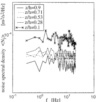
In Fig. 5 the noise spectra ^Nj& for different depths
are given. In all cases we observe a flat noise spectrum over the investigated frequency domain confirming the assumption of white noise. The level of the noise signal changes with depth. This trend is confirmed by the noise profile in Fig. 6 where its standard deviation normalized with the friction velocity has been plotted. The noise contribution increases first slowly toward the bed but increases significantly for z/h , 0.15. Also shown in Fig. 6 is the relative difference of the standard noise deviations calculated with the cross-correlation method applied to two consecutive points (Garbini et al. 1982) and the two independent vertical velocity field mea-surements, respectively. The relative difference is about 5% near the free surface and increases toward the wall where it reaches a value of 40%. The depth-averaged difference is about 20%. The disadvantage of the meth-od used by Garbini et al. (1982) is evident because it
FIG. 2. Mean velocity measurements in an open-channel flow (see Table 2 for the hydraulic flow characteristics). (a) Mean longitudinal velocity profile. (b) Universal logarithmic velocity profile. (c) Wall-law validation in the inner flow region and evaluation of the constant Br of the logarithmic profile. (d) Velocity-defect law validation andp-factor evaluation of Cole’s wake function.
FIG. 3. Comparison of the two vertical velocity variances measured in the longitudinal and transverse flow sections. The squared line shows the relative error in percent.
overestimates the noise part. It actually incorporates part of the uncorrelated but desired velocity signal between two consecutive points into the noise signal.
The same effect is also seen in Fig. 7 where the spec-trum calculated with the two point method, called
^Sj,j11&, is lower than the spectrum ^Sxy,j& at depth z/h 5
0.4. Additionally, in the inertial subrange, the slope of
^Sj,j11& is weakly increased compared to that of ^Sxy,j&.
Furthermore, in the range from 10 to 20 Hz the spectrum
^Sj,j11& becomes flat whereas the spectrum ^Sxy,j& holds
the same slope. That behaviour may originate from the overlapping of two consecutive sample volumes imply-ing an incomplete decorrelation of the noise signals.
b. Results
1) POWER SPECTRAL DENSITIES
In Figs. 8a and 8b the uncorrected and corrected pow-er spectral densities are shown for the longitudinal and transverse fluctuating velocity components at depth z/h
5 0.68. In the higher frequency domain, the
character-istic flattening of the noise-affected spectra can be dis-tinguished. As mentioned above, the contribution of the noise in the longitudinal and transverse velocity ponents is more pronounced than for the vertical com-ponent mainly because of the larger magnitude of the weighting factors due to the geometrical configuration. These factors are the same for the longitudinal and trans-verse components. Therefore the effect of noise atten-uation on the power spectra is particularly significant for both components. The slope of25/3 of the spectrum in the inertial subrange traced in Figs. 8a and 8b is followed by the two corrected spectra indicating an ef-fective correction.
FIG. 4. Power spectra of vertical fluctuating velocity and corresponding noise signals. (a) At depth z/h5 0.4. (b) At depth z/h 5 0.9. In the two figures the solid line, dash–dotted line, and dashed line represent the power spectra from the longitudinal, transverse, and cross-correlation measurements, respectively. The dotted lines show the extracted vertical noise signals.
FIG. 6. Profile of noise standard deviation relative to the friction velocity (squares). Profile of relative difference of the standard noise deviations calculated with the cross-correlation method applied to two consecutive points (Garbini et al. 1982) and the two independent vertical velocity field measurements.
FIG. 5. Power spectra of noise signals at different water depths.
2) TURBULENT INTENSITIES
Figure 9 shows the uncorrected and corrected tur-bulent intensities for each component normalized by the friction velocity. The turbulent intensity is defined as the magnitude of the turbulent velocity fluctuations. For each depth, the corrected quantities are obtained from the integration of the corresponding corrected spectra as those presented in Figs. 8a and 8b. Also drawn in
Fig. 9 are the semitheoretical curves of the turbulent intensities given by Nezu and Nakagawa (1993) as
2 Ïu9 /u* 5 2.3 exp(2z/h) 2 Ïy9 /u* 5 1.63 exp(2z/h) 2 Ïw9 /u* 5 1.27 exp(2z/h). (17) Again, the difference of the uncorrected and the cor-rected intensities of the longitudinal and the transverse components is more significant than for the vertical component. The comparison of the corrected quantities with the curves from Eq. (17) allows a certain evaluation of the efficiency of the correction method (see part 5c for the error analysis). For all three components the
FIG. 7. Spectra of the vertical fluctuating velocity component at depth z/h5 0.4. The solid line represents the result of the cross-correlation between the measurements in the longitudinal and trans-verse flow sections. The dashed line shows the result of the cross-correlation between two consecutive points as proposed by Garbini et al. (1982).
FIG. 8. Power spectra of uncorrected and corrected fluctuating velocities at depth z/h5 0.68. (a) For the longitudinal component, (b) for the transverse component. In each figure the stars represent the uncorrected data, the crosses show the corrected data.
curves are in good agreement with the measurements in the flow region z/h. 0.2.
In the range z/h, 0.2, the vertical and longitudinal intensities deviate significantly from the theoretical curves. If the comparison of the corrected data is limited
to the curves expressed by Eq. (17) these deviations could be interpreted as inaccuracies of the instrument in the wall region of the flow. However, if we consider the effect of roughness on turbulence intensities, which is not taken into account in Eq. (17), these deviations may not necessarily be the result of measurement in-accuracies.
To investigate this point further, the corresponding curves from measurements of turbulent intensities over a rough bed with a normalized roughness value of k1
s
5 85, presented by Grass (1971) using hydrogen-bubble
technique, are also plotted in Fig. 9. It can be seen that the effect of roughness is to reduce the longitudinal turbulence intensity for z/h, 0.3. The vertical intensity is less affected. It is evident that our corrected measured data are in better agreement with these curves taking into account bed roughness. The deviation of the trans-verse intensity is less important. A similar behavior was also observed by Nezu and Nakagawa (1993). It con-firms that the roughness strongly affects the longitudinal intensity for z/h , 0.3 and less so the transverse and vertical ones.
3) TURBULENT KINETIC ENERGY AND SHEAR
STRESS PROFILES
In Fig. 10 the uncorrected, the corrected turbulent kinetic energy Kj5 ( 1 1 ), and the mean
1 2 2 2
u9 y9 w9
2 j j j,l
covariance term22u9w9 are compared to the following relations:
2
K/u* 5 4.78 exp(22z/h)
2
FIG. 9. Profiles of turbulence intensities relative to the friction velocity: from the uncorrected data, from the corrected data, from the semitheoretical curves of Nezu and Nakagawa (1993) and from hydrogen-bubble technique measurements of Grass (1971).
FIG. 10. Profiles of turbulent kinetic energy relative to the friction velocity for uncorrected data, corrected data, and semitheoretical curve of Nezu and Nakagawa (1993). Profiles of shear stress relative to the friction velocity for uncorrected data and theoretical curve.
Again, the difference between the uncorrected and the corrected kinetic energy is important due to the sum of the geometrical weighting factors. The agreement of the corrected measurement with the semitheoretical predic-tion is good for z/h. 0.2. In the region z/h , 0.2, the deviation becomes more pronounced [the bottom rough-ness effect is not taken into account in Eqs. (18)].
The shear stress profile also shows a deviation of the measured profile from the theoretical prediction for z/h
, 0.2. Since this quantity is inherently not affected by
the noise signal present in the turbulent intensities [see section 2b(3)] the only remaining error source is related to the spatial averaging effect in the sample volume. However, the possible effect of bed roughness on the
shear stress in this profile range is not well documented in the literature.
4) TERMS OF THE ENERGY BALANCE EQUATION
In Fig. 11 the profiles of the different terms of the energy balance equation, all normalized by the term h/ , over the whole water depth are presented. The
un-3
u*
corrected and corrected energy dissipation rates are evaluated from the inertial subrange of the longitudinal uncorrected and corrected spectra, respectively. The fol-lowing formula is used:
21 5/3 2 3/2
FIG. 11. Profiles of normalized terms of the turbulent energy balance equation: the turbulent energy dissipation term (from the corrected and uncorrected data), the production, and corrected transport terms.
where C is the Kolmogorov constant (with a value of 0.5), and ku, Su(ku), and u92 are the longitudinal
wave-number, the longitudinal wavenumber spectrum, and the longitudinal variance, respectively. It is obvious from Fig. 8 that the uncorrected dissipation rate is largely overestimated because the 25/3 power law is not ob-served in the uncorrected spectrum. In consequence, the dissipation rate calculated from the uncorrected spec-trum is much higher than the one calculated from the corrected spectrum (Fig. 11). Good agreement is found between the corrected normalized «h/u3 and the
ex-* pression given by Nezu and Nakagawa (1993):
«h5 E (z/h)21/2
exp(23z/h), (20)
1 3
u*
where the value E1is equal to 9.8 for a Reynolds number
between 104and 105.
Also drawn in Fig. 11 are the normalized production and corrected transport terms, written as
Ph P h11 u9w9h ]u 5 5 2 3 3 3 u* 2u* u* ]z Th (T111 T 1 T )h22 33 5 3 3 u* 2u* h ] 2 2 2 5 2 3 (u9 1 y9 1 w9 )w9. (21) 2u*]z
For z/h , 0.15, the profile of the production term de-creases, which indicates an energy deficiency (the pro-duction is lower than the dissipation). This trend prob-ably confirms the inaccuracies of the measurements in that region due to the spatial averaging process in the sheared velocity domain.
In the free-surface flow region the dissipation is slightly higher than the production term, which again
is indicative for an energy deficiency. The normalized transport term is also drawn in Fig. 11 and is positive for z/h # 0.4 with a maximum value of 9. For z/h . 0.1, the corrected results are in agreement with the mea-surements found in Nezu and Nakagawa (1993). For z/h
, 0.1, this term decreases toward the wall, which again
indicates a deviation from the results found in the lit-erature.
c. Error analysis
Here we present a quantitative value of the relative differences of the corrected mean turbulence measure-ments with the above-mentioned models. The profiles of relative differences are computed for the longitudinal, transverse, and vertical turbulent intensities, the tur-bulent kinetic energy and the shear stress, noted«u,«y,
«w,«K,«uw, respectively. They are calculated as follows;
|q (z /h)c 2 q (z/h)|m
« (z/h) 5i , (22)
q (z /h)m
where qcis the corrected measured quantity and qmthe
quantity calculated from the model. Errors written with an overbar, «i, are the depth-averaged relative
differ-ences.
For z/h. 0.2, the depth-averaged values do not ex-ceed 10% (Fig. 12) (for the turbulent kinetic energy), which confirms the high accuracies of the corrected so-nar measurements.
Except for the error of the transverse turbulent in-tensity, all other errors are significant for z/h, 0.2. As mentioned before it is difficult to attribute these high values clearly to measurement inaccuracies considering that some physical process, especially the bed roughness effects, are not taken into account in the semitheoretical models.
FIG. 12. Profiles of relative errors: for the three turbulence intensities, the turbulent kinetic energy, and the shear stress. The variables written with overbars are the depth-averaged quantities (for z/h. 0.2).
6. Conclusions
A combination of two techniques to improve the pre-cision of turbulence measurements with a 3D ADVP is discussed.
The first concerns the use of a phase array emitter discussed in Hurther and Lemmin (1998).
The following improvements have been made:
R the sample volume has a constant width (;7 mm)
over a maximal distance of 60 cm from the emitter
R the effect of the beam divergence (or phase distortion
of the front wave), appearing as an additional noise variance in the measurements, can no longer be dis-tinguished on beam measurements
R spatial averaging effect is considerably reduced and
is only dependent on flow characteristics in the ver-tical flow direction since the emitter’s normalized di-rectivity function is no longer a function of the water depth.
The second technique used to increase the signal-to-noise ratio of the measurements is a direct correction method of the Doppler signal. It has been verified that the following noise signal characteristics apply to the method
R the noise has a flat spectrum independent of the flow
depth
R the noise signal is uncorrelated from the velocity
sig-nal
R the noise signal is uncorrelated between the different
receivers
R the receivers and the different analogic circuitries can
be considered as identical.
Based on these results it is possible to apply the cor-rection method. It consists in making a redundant mea-surement of the instantaneous vertical velocity field with
two independent working tristatic subsystems in the lon-gitudinal and transverse flow sections. By calculating the difference between the magnitudes of the auto- and cross-spectra we rebuild the noise spectra of each ve-locity component by considering the specific geomet-rical configuration. Thereby, the following mean tur-bulence quantities were corrected:
R the three turbulence intensities (with a mean relative
error of;5% in the outer flow domain)
R the turbulent kinetic energy (with a mean relative error
of;9% in the outer flow domain)
R the turbulence spectra over the entire resolved
fre-quency band
R the turbulent energy dissipation rate, which is of
par-ticular importance if energy balances are investigated. From comparisons of the corrected data with raw data and with results from literature, we have shown quan-titatively that the corrected ADVP data are highly re-liable and accurate in the flow region z/h . 0.2. This result is of major importance for our further investi-gations concerning free surface turbulence in open-channel flow based on 3D-ADVP velocity field mea-surements. Therefore the presented method has been programmed as a systematic correction method of the sonar measurements. Another advantage of the proposed technique is that it does not require assumptions about the flow characteristics. As a result the presented so-lution can be applied to any ADVP applications as long as the geometrical configuration permits a simultaneous redundant velocity component measurement. Voulgaris and Throwbridge (1998) have mentioned in their con-clusion that the presence of high noise terms is an in-escapable feature of the geometry of an ADV. This re-mark is valid for their case. We have shown here that with another geometrical configuration and an
appro-priate signal treatment the noise contribution to the mean turbulence terms can be eliminated.
Supplementary studies are needed to quantitatively evaluate the ‘‘true’’ precision of sonar measurements in the wall region of an open-channel flow. From theo-retical considerations (which are difficult to validate ex-perimentally), we allocate the remaining deviations (in the wall region) of the corrected measurements to effects of the spatial averaging since no other noise process is identified after application of the presented correction method. However, effects of bottom roughness cannot be excluded either.
Acknowledgments. Comments by two anonymous
re-viewers helped to improve the presentation. This work was funded by the Swiss National Science Foundation grant 20-39494.93. We are grateful for the support.
REFERENCES
Cabrera, R., K. Deines, B. Brumley, and E. Terray, 1987: Develop-ment of a practical coherent acoustic Doppler current profiler. Proc. Oceans ’87. The Ocean, An International Workplace, Hal-ifax, NS, Canada, IEEE, 93–97.
Garbini, J. L., F. K. Forster, and J. E. Jorgensen, 1982: Measurement
of fluid turbulence based on pulsed ultrasound techniques. Part 1. Analysis. J. Fluid Mech., 118, 445–470.
Graf, W. H., and M. Altinakar, 1998: Fluvial Hydraulics. Wiley & Sons Ltd., 681 pp.
Grass, A. J., 1971: Structural features of turbulent flow over smooth and rough boundaries. J. Fluid Mech., 50, 233–255.
Hurther, D., and U. Lemmin, 1998: A constant beamwidth transducer for 3D acoustic Doppler profile measurements in open channel flows. Meas. Sci. Technol., 9, 1706–1714.
Lemmin, U., and T. Rolland, 1997: An acoustic velocity profiler for laboratory and field studies. J. Hydraul. Eng., 123, 1089–1098. Lhermitte, R., and U. Lemmin, 1994: Open-channel flow and tur-bulence measurement by high-resolution Doppler sonar. J. At-mos. Oceanic Technol., 11, 1295–1308.
Lohrmann, A., R. Cabrera, and N. C. Kraus, 1995: Direct measure-ments of Reynolds stress with an acoustic Doppler velocimeter. Proc. IEEE Fifth Conf. on Current Measurements, St. Peters-burg, FL, IEEE Oceanic Engineering Society, 205–210. Nezu, I., and H. Nakagawa, 1993: Turbulence in open channel flows.
AIHR Monogr. Series, No. 4, Balkema, 281 pp.
Rolland, T., 1994: De´veloppement d’une instrumentation Doppler ul-trasonore adapte´e a` l’e´tude hydraulique de la turbulence dans les canaux. Ph.D. dissertation 1281, Swiss Federal Institute of Technology–Lausanne, 155 pp.
Shen, C., and U. Lemmin, 1997: Ultrasonic scattering in highly tur-bulent clear water flow. Ultrasonics, 35, 57–64.
Voulgaris, G., and J. H. Trowbridge, 1998: Evaluation of the acoustic Doppler velocimeter (ADV) for turbulence measurements. J. At-mos. Oceanic Technol., 15, 272–289.
Zedel, L., A. E. Hay, and A. Lohrmann, 1996: Performance of a single beam pulse-to-pulse coherent Doppler profiler. IEEE J. Oceanic Eng., 21, 290–297.