A robust and parsimonious regional disaggregation method for deriving hourly rainfall intensities for the UK

(1)

HAL Id: hal-00298664

https://hal.archives-ouvertes.fr/hal-00298664

Submitted on 14 Jun 2005

HAL is a multi-disciplinary open access

archive for the deposit and dissemination of sci-entific research documents, whether they are pub-lished or not. The documents may come from teaching and research institutions in France or abroad, or from public or private research centers.

L’archive ouverte pluridisciplinaire HAL, est destinée au dépôt et à la diffusion de documents scientifiques de niveau recherche, publiés ou non, émanant des établissements d’enseignement et de recherche français ou étrangers, des laboratoires publics ou privés.

A robust and parsimonious regional disaggregation

method for deriving hourly rainfall intensities for the

UK

D. Maréchal, I. P. Holman

To cite this version:

D. Maréchal, I. P. Holman. A robust and parsimonious regional disaggregation method for deriving hourly rainfall intensities for the UK. Hydrology and Earth System Sciences Discussions, European Geosciences Union, 2005, 2 (3), pp.1047-1065. �hal-00298664�

(2)

HESSD

2, 1047–1065, 2005 A robust and parsimonious regional disaggregation method D. Mar ´echal and

I. P. Holman Title Page Abstract Introduction Conclusions References Tables Figures J I J I Back Close

Full Screen / Esc

Print Version Interactive Discussion Hydrol. Earth Sys. Sci. Discuss., 2, 1047–1065, 2005

www.copernicus.org/EGU/hess/hessd/2/1047/ SRef-ID: 1812-2116/hessd/2005-2-1047 European Geosciences Union

Hydrology and Earth System Sciences Discussions

Papers published in Hydrology and Earth System Sciences Discussions are under open-access review for the journal Hydrology and Earth System Sciences

A robust and parsimonious regional

disaggregation method for deriving

hourly rainfall intensities for the UK

D. Mar ´echal1, 2and I. P. Holman1

1

Institute of Water and Environment, Cranfield University, Silsoe, Bedford, UK

2

now at: EQECAT, 16 Rue Drouot 75009 Paris, France

Received: 9 May 2005 – Accepted: 25 May 2005 – Published: 14 June 2005 Correspondence to: I. P. Holman (i.holman@cranfield.ac.uk)

(3)

HESSD

Full Screen / Esc

Print Version Interactive Discussion

Abstract

A regional rainfall disaggregation method from daily to hourly intensities is presented for the entire UK, which was developed for use with regionalised hydrological and water quality models. The approach is based on the inter-dependence of the hourly rainfall intensities during a rainfall event. The analysis of 23 229 days with at least 15 mm

5

of precipitation from 238 weather stations throughout the UK allowed regional param-eters for climatically homogeneous regions of the UK to be derived for each season. The method reproduces well the main statistical characteristics of the data (mean, min-imum and maxmin-imum intensity and standard deviation). The method is fully operational, computationally efficient and can be applied to any location throughout the UK.

10

1. Introduction

Water quality legislation is increasingly requiring standardized approaches to manage-ment and monitoring across regions and countries. Regionalised models (e.g. nitrates: Lord and Anthony, 2000; pesticides: Holman et al., 2004; erosion: Brazier et al., 2001; phosphorus: Hutchins et al., 2002) are an important tool for helping comply with

leg-15

islation in a cost-effective manner, allowing ex ante evaluation of the effectiveness and consequences of environmental and agricultural policy measures. Many of these mod-els tend to operate on a daily timestep, combining the mechanisms of infiltration-excess and saturation-excess runoff generation into a single process. Although infiltration ex-cess surface runoff is generally accepted as being less important in humid and

temper-20

ate regions, it is becoming increasingly apparent that it can be an important process in a wide range of soils (Evans 1996) due to land use changes or to farming practices which impact on the infiltration characteristics of the soil (Holman et al., 2003). How-ever, in many countries there are insufficient numbers of rainfall stations recording the necessary sub-daily data to directly allow national-scale simulation. For example, the

25

Meteorological Office in the UK runs a network of more than 5000 rainfall stations, but 1048

(4)

HESSD

Full Screen / Esc

Print Version Interactive Discussion hourly rainfall data are only collected for a few hundred stations.

One solution to obtain fine temporal resolution rainfall data is to disaggregate the coarse (e.g. daily) data. Disaggregation is achieved by applying stochastic rainfall models to reproduce the main statistics of the data. The two main categories of such stochastic models are profile-based (e.g. Hershenhorn and Woolhiser, 1987;

Kout-5

soyiannis and Xanthopoulos, 1990) and pulse-based (e.g. Onof and Wheater, 1993; Cowpertwait et al., 1996a) rainfall models, but all were developed for use with individ-ual station data (Cameron et al., 2000) which are inappropriate for regional or national studies.

Only a few attempts have been made to derive regional parameters for stochastic

10

rainfall models. Econopouly et al. (1990) found that it was possible to export the cal-ibrated Hershenhorn and Woolhiser (1987) model over a long distance in the United States of America if the condition of climatic similarity was respected. Gyasi-Agyei (1999) tried to compute regional parameters in Australia for the Gyasi-Agyei – Willgo-ose model. Cowpertwait et al. (1996b) derived regional parameters for Great Britain but

15

used only 27 sites with hourly records. Koutsoyiannis et al. (2003) presented a method-ology for spatial-temporal disaggregation aimed at generating hourly rainfall series for several sites from daily rainfall series from all the sites and hourly rainfall series from at least one site.

These methods showed the promise of regional rainfall disaggregation but failed to

20

propose robust operational methods because of the complexity of multi-site parameter estimation (Kottegoda et al., 2003; Favre et al., 2002). Nevertheless robust, compu-tationally efficient regionalised disaggregation methodologies will be required for water quality modelling to support regional and national policy. The aim of this study is there-fore to develop a robust and parsimonious rainfall disaggregation method from daily to

25

hourly intensities that is applicable throughout the UK.

(5)

HESSD

Full Screen / Esc

2. Data set

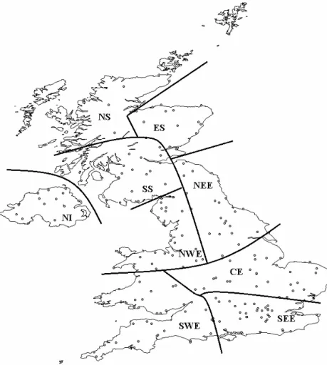
A total of 389 stations spread over England, Wales, Scotland and Northern Ireland corresponding to 5798 station/years with hourly rainfall data between 1983 and 1999 have been analysed. Only intense rainfall episodes have been selected, defined as days (from 09:00 a.m. to 09:00 a.m.) when the total daily rainfall was ≥15 mm. Table 1

5

summarises the distribution of the 23 229 intense events and 238 stations for the 9 homogeneous regions (Fig. 1) defined following Gregory et al. (1991).

3. Statistical analysis

Meteorological processes may vary depending on the period of the year (Guntner et al., 2001), but the small number of intense rainfall events for the summer months in some

10

regions necessitated the aggregation of several months to get significant samples of data. Consequently the analysis has been carried out for 4 seasons (winter: January– March; spring: April–June; Summer: July–September; Autumn: October–December) in the 9 regions.

3.1. Analysis strategy

15

Let h_k be the dimensionless hourly rainfall intensity at hour k in its discrete form:

h_k = qk n P j=1 q_j (1)

where q is the observed hourly intensity in mm/h and n the length of the rainfall event. In this study, the adopted approach is equivalent to assume that there was only one

(6)

HESSD

Full Screen / Esc

Print Version Interactive Discussion rainfall event per day, Eq. (1) becomes:

h_k = qk 24 P j=1 q_j (2)

The dimensionless hyetograph expresses the dimensionless accumulated quantity of rainfall after k hours.

H_k = k X j=1 h_j = k P j=1 q_j 24 P j=1 q_j (3) 5

Kottegoda et al. (2003) and Garcia-Guzman and Aranda-Oliver (1993) suggested that the successive values of H_k were not independent. We propose here to describe this dependence of the dimensionless hourly rainfall intensities by representing the dimensionless intensity during the most intense hour by a statistical distribution, and by defining explicit relationships between the dimensionless intensities during the most

10

intense hour and the other hours (Boughton, 2000). 3.2. Hour of maximum rainfall

The 24 hourly rainfall intensities are classified from the most intense hour to the least intense hour and noted as q₁ to q₂₄. h₁ is derived from Eq. (2) and then represented by a statistical distribution covering all rainfall events in the climatically homogeneous

15

region. It was hypothesised that h₁was best described by the Log-Normal distribution (Fig. 2), which was assessed using a Kolmogorov-Smirnov two-sample test. In 81% of the 36 Kolmogorov-Smirnov tests (9 climate zones and 4 seasons) the hypothesis could not be rejected at α=0.05, and in 95 % of the cases at the 0.01 level. The Log-Normal distribution was therefore adopted as the best description of the dimensionless

20

(7)

HESSD

Full Screen / Esc

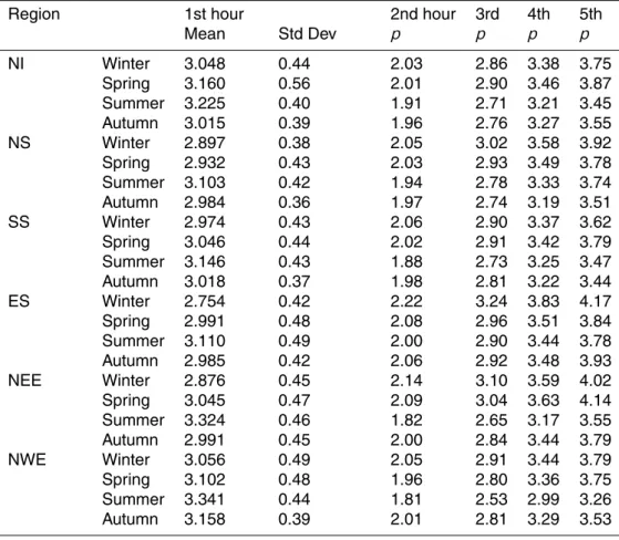
Print Version Interactive Discussion intensity of the hour of maximal rainfall. Values of the mean and the standard deviation

of the Log-Normal distributions for the climatic region-season combinations are given in Table 2.

The fitted mean and standard deviations of the Log-Normal distributions show re-gional variations due to the climatic variations over the UK, corroborating the climatic

5

regions used. In the summer, the fitted mean values increase from west to east asso-ciated with a transition from rainfall assoasso-ciated with Atlantic depressions, which create frontal precipitation events with a moderate intensity over rather long periods, to con-vectional events generating heavy showers and thunderstorms. In winter periods the reverse is true with fitted mean values decreasing eastwards. The UK is the first land

10

met by Atlantic fronts which get weaker as they move east. In all regions the mean values have their maximum for the summer period and their minimum for the winter. Consequently, these seasonal variations are more severe for the eastern regions than the western regions where the precipitation events are more stable in both amount and type.

15

3.3. Other 23 intensities

The other 23 dimensionless intensities h_k are directly related to the rainfall amount during more intense hours:

h_k = qk 24 P j₌₁ q_j = rk∗   k−1 X j=1 h_j   (4)

with k the hour number between 2 and 24 and r_k:

20 r_k = qk k−1 P j=1 q_j (5) 1052

(8)

HESSD

Full Screen / Esc

Print Version Interactive Discussion It was found that the best type of regression to express the relationship between rainfall

depths r_kand h₁, h₂. . . , h_k₋₁is exponential (Fig. 3). h_kis therefore expressed as:

h_k = −       k−1 P j₌₁ h_j p       ln       k−1 P j₌₁ h_j 100       (6)

Values of p for the 2nd to 5th hours are given in Table 2. The distributions of the coefficients of determination for the regressions are graphically presented in Fig. 4 for

5

the 2nd, 3rd, 4th and 5th hours. These coefficients of determination tend to improve towards the less intense rain hours as the information on the shape of the hyetograph held by previous hours increases.

4. Evaluation

The disaggregation method was evaluated for the 9 climate regions of the UK. The

10

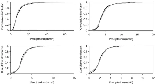
relative intensities of the first hours were selected randomly from the calibrated Log-Normal distributions and then the intensities in subsequent hours were derived using the correlation formulae. As an example, Fig. 5 compares the observed and predicted rainfall intensities for the Central England region in summer for the first 4 h. The evalu-ation tested whether the disaggregevalu-ation method reproduces the standard and extreme

15

statistics (Cameron et al., 2000) of the observations for each hour.

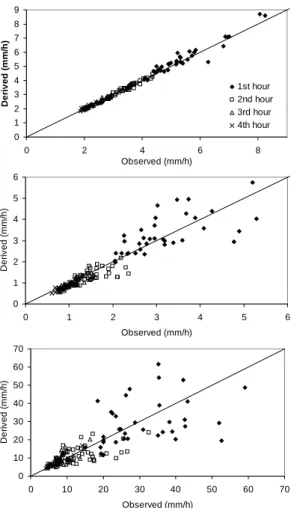
Because the disaggregation method outputs rainfall intensities and not time series, the analysis was limited to the mean intensity, standard deviation, maximum and min-imum dimensionless intensities. The minmin-imum dimensionless intensity is well repro-duced. Figure 6 shows the results for the mean intensity, standard deviation and

maxi-20

mum dimensionless intensity for the first 4 h.

(9)

HESSD

Full Screen / Esc

Print Version Interactive Discussion The two-sample t test was used to determine if the observed and predicted

inten-sities were drawn from populations with the same mean. In 90% of the cases the hypothesis could not be rejected at the 5% level for the first 4 h. Although, this pro-portion deteriorated for the 5th hour, when the hypothesis could not be rejected in only 45% of the cases, the rainfall intensities are unlikely to be significant for generating

5

infiltration-excess runoff.

The standard deviation is generally well predicted, it is only slightly underestimated for the highest intensities of the first and second hours. The prediction of the maximum hourly intensities was also generally good, although a greater dispersion of the predic-tions for the high events above 30 mm/h around the 1:1 line was observed (Fig. 8).

10

Globally, this disaggregation method proves to be robust and to give satisfactory results.

5. Conclusions

A robust and parsimonious disaggregation method from daily to hourly rainfall inten-sities applicable in homogeneous regions of the UK for water resources modelling is

15

presented. The method assumes that the intensity during the most intense hour dic-tates the type of rainfall event and therefore the intensities during the other 23 h of the day. Consequently, these 23 fractions are directly related to the rainfall amount falling during more intense hours. 23 229 days with at least 15 mm of precipitation from 238 meteorological stations spread over the UK were analysed. In 81% of the cases the

20

Log-Normal distribution represents well the relative rainfall intensities during the most intense hour, and that the relations between rainfall depths are well explained using an exponential regression.

An evaluation of its capability to reproduce the main statistics of the data concluded that it is successful for its purpose for water resources modelling, although it showed

25

some discrepancies with the observations for the infrequent very intense events. Nev-ertheless the significant advantages of the proposed method are: 1) its national

(10)

HESSD

Full Screen / Esc

Print Version Interactive Discussion cability, as all parameters have been determined for 9 regions dividing the UK, and 2)

its extreme simplicity of use.

Acknowledgements. This work was funded by the European Commission Framework V

Pro-gramme as part of the MULINO project (EVK1-2000-22089). Thanks are due to the British Atmospheric Data Centre for providing access to the UK Meteorological Office Land Surface

5

Observation Stations Data and to the UK Meteorological Office for the use of their data.

References

Brazier, R. E., Rowan, J. S., Anthony, S. G., and Quinn, P.F.: “MIRSED” towards an MIR approach to modelling hillslope soil erosion at the national scale, 42, 59–79, 2001.

Cameron, D., Beven, K., and Tawn, J.: An evaluation of three stochastic rainfall models, J.

10

Hydrol., 228, 130–149, 2000.

Cameron, D., Beven, K., Tawn, J., and Naden, P.: Flood frequency estimation by continuous simulation (with likelihood based uncertainty estimation), Hydrol. Earth Sys. Sci., 4, 23–34, 2000,SRef-ID: 1607-7938/hess/2000-4-23.

Boughton, W.: A model for disaggregating daily to hourly rainfalls for design flood estimation,

15

Cooperative Research Centre for Catchment Hydrology (CRCCH), Tech. Rep. 00/15,http: //www.catchment.crc.org.au/pdfs/technical200015.pdf, 2000.

Cowpertwait, P. S. P., O’Connell, P. E., Metcalfe, A. V., and Mawdsley, J. A.: Stochastic point process modelling of rainfall, I Single-site fitting and validation, J. Hydrol., 175, 17–46, 1996a. Cowpertwait, P. S. P., O’Connell, P. E., Metcalfe, A. V., and Mawdsley, J. A.: Stochastic point

20

process modelling of rainfall, I Regionalisation and disaggregation, J. Hydrol., 175, 47–65, 1996b.

Econopouly, T. W., Davis, D. R., and Woolhiser, D. A.: Parameter transferability for a daily rainfall disaggregation model, J. Hydrol., 118, 209–228, 1990.

Evans, R.: Soil erosion and its impacts in England and Wales, Friends of the Earth, London,

25

121, 1996.

Favre, A. C., Musy, A., and Morgenthaler, S.: Two-site modeling of rainfall based on the Neyman-Scott process, Wat. Res. Res., 38, 1307–1313, 2002.

Garcia-Guzman, A. and Aranda-Oliver, E.: A stochastic model of dimensionless hyetograph, Wat. Res. Res., 29, 2363–2370, 1993.

30

(11)

HESSD

Full Screen / Esc

Gregory, J. M., Jones, P. D., and Wigley, T. M. L.: Precipitation in Britain: an analysis of area-average data updated to 1989, Int. J. of Climatol.. 11, 331–345, 1991.

Guntner, A., Olsson, J., Calver, A., and Gannon, B.: Cascade-based disaggregation of con-tinuous rainfall time series: the influence of climate, Hydrol. Earth Sys. Sci., 5, 145–164, 2001.

5

Gyasi-Agyei, Y.: Identification of regional parameters of a stochastic model for rainfall disag-gregation, J. Hydrol., 223, 148–163, 1999.

Hershenhorn, J. and Woolhiser, D. A.: Disaggregation of daily rainfall, J. Hydrol., 95, 299–322, 1987.

Holman, I. P., Hollis, J. M., Bramley, M. E., and Thompson, T. R. E.: The contribution of soil

10

structural degradation to catchment flooding: a preliminary investigation of the 2000 floods in England and Wales, Hydrol. Earth Sys. Sci., 7, 754–765, 2003,

SRef-ID: 1607-7938/hess/2003-7-754.

Holman, I. P., Dubus, I. G., Hollis, J. M., and Brown, C. D.: Using a linked soil model emulator and unsaturated zone leaching model to account for preferential flow when assessing the

15

spatially distributed risk of pesticide leaching to groundwater in England and Wales, Science of the Total Environment, 318, 73–88, 2004.

Hutchins, M. G., Anthony, S. G., Hodgkinson, R. A., and Withers, P. J. A: Modularised process-based modelling of phosphorus loss at farm and catchment scale, Hydrol. Earth Sys. Sci., 6, 1017–1030, 2002,SRef-ID: 1607-7938/hess/2002-6-1017.

20

Kottegoda, N. T., Natale, L., and Raiteri, E.: A parsimonious approach to stochastic multisite modelling and disaggregation of daily rainfall, J. Hydrol., 274, 47–61, 2003.

Koutsoyiannis, D. and Xanthopoulos, T.: A dynamic model for short-scale rainfall disaggrega-tion, Hydrol. Sci. J., 35, 305–322, 1990.

Koutsoyiannis, D. Onof, C., and Wheater, H. S.: Multivariate rainfall disaggregation at a fine

25

timescale, Wat. Res. Res., 39, 1173–1190, 2003.

Lord, E. I., Anthony, S. G.: MAGPIE: A modelling framework for evaluating nitrate losses at national and catchment scales, Soil Use Manage, 16, 167–174 Suppl., 2000.

Onof, C. and Wheater, H. S.: Modelling of British rainfall using a random parameter Barlett-Lewis rectangular pulse model, J. Hydrol., 149, 67–95, 1993.

30

(12)

HESSD

Full Screen / Esc

Print Version Interactive Discussion Table 1. Distribution of the meteorological stations and rainfall events.

Region Number of Stations Number of events

Northern Ireland(NI) 15 942

North of Scotland (NS) 21 3284

East of Scotland (ES) 16 1241

South of Scotland (SS) 32 4443

North West England (NWE) 14 1689

North East England (NEE) 22 1107

South West England (SWE) 49 5260

Central England (CE) 28 2089

South East of England (SEE) 41 3216

Total 238 23 229

(13)

HESSD

Full Screen / Esc

Print Version Interactive Discussion Table 2. Regionalised seasonal parameter values for the UK.

Region 1st hour 2nd hour 3rd 4th 5th

Mean Std Dev p p p p NI Winter 3.048 0.44 2.03 2.86 3.38 3.75 Spring 3.160 0.56 2.01 2.90 3.46 3.87 Summer 3.225 0.40 1.91 2.71 3.21 3.45 Autumn 3.015 0.39 1.96 2.76 3.27 3.55 NS Winter 2.897 0.38 2.05 3.02 3.58 3.92 Spring 2.932 0.43 2.03 2.93 3.49 3.78 Summer 3.103 0.42 1.94 2.78 3.33 3.74 Autumn 2.984 0.36 1.97 2.74 3.19 3.51 SS Winter 2.974 0.43 2.06 2.90 3.37 3.62 Spring 3.046 0.44 2.02 2.91 3.42 3.79 Summer 3.146 0.43 1.88 2.73 3.25 3.47 Autumn 3.018 0.37 1.98 2.81 3.22 3.44 ES Winter 2.754 0.42 2.22 3.24 3.83 4.17 Spring 2.991 0.48 2.08 2.96 3.51 3.84 Summer 3.110 0.49 2.00 2.90 3.44 3.78 Autumn 2.985 0.42 2.06 2.92 3.48 3.93 NEE Winter 2.876 0.45 2.14 3.10 3.59 4.02 Spring 3.045 0.47 2.09 3.04 3.63 4.14 Summer 3.324 0.46 1.82 2.65 3.17 3.55 Autumn 2.991 0.45 2.00 2.84 3.44 3.79 NWE Winter 3.056 0.49 2.05 2.91 3.44 3.79 Spring 3.102 0.48 1.96 2.80 3.36 3.75 Summer 3.341 0.44 1.81 2.53 2.99 3.26 Autumn 3.158 0.39 2.01 2.81 3.29 3.53 1058

(14)

HESSD

Full Screen / Esc

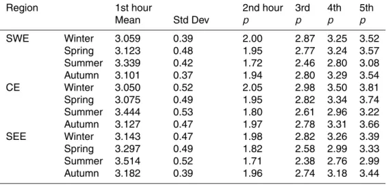
Print Version Interactive Discussion Table 2. Continued.

Region 1st hour 2nd hour 3rd 4th 5th

Mean Std Dev p p p p SWE Winter 3.059 0.39 2.00 2.87 3.25 3.52 Spring 3.123 0.48 1.95 2.77 3.24 3.57 Summer 3.339 0.42 1.72 2.46 2.80 3.08 Autumn 3.101 0.37 1.94 2.80 3.29 3.54 CE Winter 3.050 0.52 2.05 2.98 3.50 3.81 Spring 3.075 0.49 1.95 2.82 3.34 3.74 Summer 3.444 0.53 1.80 2.61 2.96 3.22 Autumn 3.127 0.47 1.97 2.78 3.31 3.66 SEE Winter 3.143 0.47 1.98 2.82 3.26 3.39 Spring 3.297 0.49 1.82 2.58 2.99 3.33 Summer 3.514 0.52 1.71 2.38 2.76 2.99 Autumn 3.182 0.39 1.96 2.74 3.18 3.44 1059

(15)

HESSD

Full Screen / Esc

EGU

Figure 1. The homogenous climate regions (adapted from Gregory et al., 1991) and the location of the meteorological stations providing hourly data

Fig. 1. The homogenous climate regions (adapted from Gregory et al., 1991) and the location

of the meteorological stations providing hourly data.

(16)

HESSD

Full Screen / Esc

EGU Figure 2. Distribution of the relative rainfall intensity of the 1st hour h1 – Central

England region in spring

Fig. 2. Distribution of the relative rainfall intensity of the 1st hour h₁ – Central England region in spring.

(17)

HESSD

Full Screen / Esc

Print Version Interactive Discussion EGU R2 = 0.58 0 10 20 30 40 50 60 70 80 90 100 0 10 20 30 40 50 60 70 80 90 100 r2 (% of R1) R1 ( % of d a ily to ta l)

Figure 3. Regression analysis of the relative rainfall intensity of the 2nd hour r2 –

spring CE region

Fig. 3. Regression analysis of the relative rainfall intensity of the 2nd hour r₂ – spring CE region.

(18)

HESSD

Full Screen / Esc

Print Version Interactive Discussion EGU 0 5 10 15 20 25 30 0 0.1 0.2 0.3 0.4 0.5 0.6 0.7 0.8 R2 N u m b er o f valu es ( % ) 0 5 10 15 20 25 30 0 0.1 0.2 0.3 0.4 0.5 0.6 0.7 0.8 R2 Nu m b e r o f valu es ( % ) 0 5 10 15 20 25 30 0 0.1 0.2 0.3 0.4 0.5 0.6 0.7 0.8 R2 Nu m b er o f valu es ( % ) 0 5 10 15 20 25 30 0 0.1 0.2 0.3 0.4 0.5 0.6 0.7 0.8 R2 Nu m b er o f va lu es ( % )

Figure 4. Distribution of the coefficients of determination for top left) 2nd_{hour, top}

right) 3rd hour, lower left) 4th hour and lower right) 5th hour for all climatic regions

and seasons

Fig. 4. Distribution of the coefficients of determination for top left: 2nd hour, top right: 3rd hour,

lower left: 4th hour and lower right: 5th hour for all climatic regions and seasons.

(19)

HESSD

Full Screen / Esc

Print Version Interactive Discussion EGU 0 0.2 0.4 0.6 0.8 1 0 20 40 60 Precipitation (mm/h) C u m u la ti ve d ist ri b u tio n 0 0.2 0.4 0.6 0.8 1 0 5 10 15 20 Precipitation (mm/h) C u m u la ti ve d ist ri b u tio n 0 0.2 0.4 0.6 0.8 1 0 5 10 15 Precipitation (mm/h) C u m u la ti v e d is tr ibu ti o n 0 0.2 0.4 0.6 0.8 1 0 2 4 6 8 10 12 Precipitation (mm/h) C u m u la ti v e d is tr ibu ti o n

Figure 5. Comparison of observed (grey line) and predicted (black line) rainfall intensities for top left) the 1st hour, top right) the 2nd hour, lower left) the 3rd hour and lower right) the 4th_{hour – Central England region in summer}

Fig. 5. Comparison of observed (grey line) and predicted (black line) rainfall intensities for top

left: the 1st hour, top right: the 2nd hour, lower left: the 3rd hour and lower right: the 4th hour – Central England region in summer.

(20)

HESSD

Full Screen / Esc

Print Version Interactive Discussion 18 0 1 2 3 4 5 6 7 8 9 0 2 4 6 8 Observed (mm/h) Der iv e d ( m m /h) 1st hour 2nd hour 3rd hour 4th hour 0 1 2 3 4 5 6 0 1 2 3 4 5 6 Observed (mm/h) D e riv e d (m m /h ) 0 10 20 30 40 50 60 70 0 10 20 30 40 50 60 70 Observed (mm/h) D e riv e d (m m /h )

Figure 6. Comparison of predicted vs observed (top) hourly mean intensities, (middle) standard deviation of hourly mean intensities and (lower) maximum hourly intensities for all climatic regions

Fig. 6. Comparison of predicted vs observed (top) hourly mean intensities, (middle) standard

deviation of hourly mean intensities and (lower) maximum hourly intensities for all climatic re-gions.