HAL Id: hal-00296310
https://hal.archives-ouvertes.fr/hal-00296310
Submitted on 16 Aug 2007
HAL is a multi-disciplinary open access
archive for the deposit and dissemination of
sci-entific research documents, whether they are
pub-lished or not. The documents may come from
teaching and research institutions in France or
abroad, or from public or private research centers.
L’archive ouverte pluridisciplinaire HAL, est
destinée au dépôt et à la diffusion de documents
scientifiques de niveau recherche, publiés ou non,
émanant des établissements d’enseignement et de
recherche français ou étrangers, des laboratoires
publics ou privés.
Observations of OH and HO2 radicals in coastal
Antarctica
W. J. Bloss, J. D. Lee, D. E. Heard, R. A. Salmon, S. J.-B. Bauguitte, H. K.
Roscoe, A. E. Jones
To cite this version:
W. J. Bloss, J. D. Lee, D. E. Heard, R. A. Salmon, S. J.-B. Bauguitte, et al.. Observations of OH
and HO2 radicals in coastal Antarctica. Atmospheric Chemistry and Physics, European Geosciences
Union, 2007, 7 (16), pp.4171-4185. �hal-00296310�
www.atmos-chem-phys.net/7/4171/2007/ © Author(s) 2007. This work is licensed under a Creative Commons License.
Chemistry
and Physics
Observations of OH and HO
2
radicals in coastal Antarctica
W. J. Bloss1,*, J. D. Lee1,**, D. E. Heard1, R. A. Salmon2, S. J.-B. Bauguitte2, H. K. Roscoe2, and A. E. Jones2 1School of Chemistry, University of Leeds, Woodhouse Lane, Leeds, LS2 9JT, UK
2British Antarctic Survey, Madingley Road, Cambridge, CB3 0ET, UK
*now at: School of Geography, Earth & Environmental Sciences, University of Birmingham, Edgbaston, Birmingham, B15
2TT, UK
**now at: Department of Chemistry, University of York, Heslington, York, YO10 5DD, UK
Received: 18 January 2007 – Published in Atmos. Chem. Phys. Discuss.: 23 February 2007 Revised: 27 July 2007 – Accepted: 10 August 2007 – Published: 16 August 2007
Abstract. OH and HO2 radical concentrations have been
measured in the boundary layer of coastal Antarctica for a six-week period during the austral summer of 2005. The measurements were performed at the British Antarctic Sur-vey’s Halley Research Station (75◦35′S, 26◦19′W), using the technique of on-resonance laser-induced fluorescence to detect OH, with HO2measured following chemical
conver-sion through addition of NO. The mean radical levels were 3.9×10⁵molecule cm−3for OH, and 0.76 ppt for HO2(ppt
denotes parts per trillion, by volume). Typical maximum (local noontime) levels were 7.9×10⁵ molecule cm−3 and 1.50 ppt for OH and HO2respectively. The main sources of
HOxwere photolysis of O3and HCHO, with potentially
im-portant but uncertain contributions from HONO and higher aldehydes. Of the measured OH sinks, reaction with CO and CH4 dominated, however comparison of the observed
OH concentrations with those calculated via the steady state approximation indicated that additional co-reactants were likely to have been present. Elevated levels of NOxresulting
from snowpack photochemistry contributed to HOxcycling
and enhanced levels of OH, however the halogen oxides IO and BrO dominated the CH3O2 – HO2– OH conversion in
this environment, with associated ozone destruction.
1 Introduction
The chemistry of the sunlit troposphere is dominated by the reactions of the hydroxyl radical, OH, which is responsi-ble for initiating the degradation of most hydrocarbons and other species emitted to the atmosphere. Knowledge of at-mospheric hydroxyl levels, of related species such as HO2,
and the chemical processes which govern their abundance, is central to explaining current atmospheric trace gas distribu-tions and predicting their likely future evolution.
Correspondence to: W. J. Bloss ([email protected])
Field measurement campaigns, in which coordinated mea-surements of radical species such as OH, HO2, NO etc. have
been performed, provide a means to test and refine our un-derstanding of fast radical photochemistry. Measurements of OH and HO2 radicals have been performed in a range
of marine and continental, polluted and clean environments (e.g. Heard and Pilling, 2003, and references therein); how-ever very few measurements have been performed in the po-lar boundary layer, where the differing physical conditions together with snowpack emission and deposition processes give rise to a unique chemical environment.
Interest in the chemistry of the polar boundary layer, and the atmospheric chemistry above the surface of the polar ice sheets and sea ice, has grown in recent years, driven in part by interest in understanding atmospheric evolution through measurements of trace gases in air trapped in ice cores and firn. In addition to climatic information derived from long-lived tracers such as CO2levels and various
iso-tope ratios, measurements of sulphur, nitrate and perox-ide levels have all been used to infer historic atmospheric composition (e.g. Legrand and Mayewski, 1997, and ref-erences therein); understanding the chemical environment in which these species are deposited and incorporated in firn/ice, i.e. the background chemistry of the polar boundary layers, is clearly important for such analyses.
From the perspective of the modern atmosphere, interest in the polar boundary layer has also been driven by the ob-servation of periodic surface ozone depletion events linked to bromine chemistry in the arctic, and the recognition that snowpack can act as a source of nitrogen oxides NO and NO2
(collectively NOx), HONO, HCHO and peroxides, amongst
other species, thereby modifying the boundary layer compo-sition from what might be expected for regions remote from pollutant sources.
In the sunlit background troposphere, radical production is driven primarily by the short-wavelength photolysis of ozone, and reaction of the electronically excited O(1D) atoms
2
so formed with water vapour (in competition with quench-ing), forming hydroxyl radicals:
O3+hv → O(1D) + O2 (R1)
O(1D) + H2O → OH + OH (R2)
OH subsequently reacts with hydrocarbons such as methane, and with carbon monoxide, forming organic and hydroper-oxy radicals respectively:
OH + CH4(+O2) → CH3O2(+H2O) (R3)
OH + CO(+O2) → HO2(+CO2) (R4)
The fate of the peroxy radicals depends upon the level of NOx(=[NO] + [NO2]). In clean (low NOx) conditions, the
peroxy radicals largely undergo self- or cross-reaction, lead-ing to the formation of peroxides, alcohols and aldehydes, and in very low NOx environments, ozone destruction
re-sults (via Reaction R1). Alternatively, peroxy radicals may react with NO, converting CH3O2 into HO2 (and HCHO),
and HO2into OH, with associated NO to NO2conversion:
CH3O2+NO(+O2) → HCHO + NO2+HO2 (R5)
HO2+NO → OH + NO2 (R6)
NO2in turn readily undergoes photolysis in the lower
atmo-sphere leading to the formation of ozone.
NO2+hv → NO + O (R7)
O + O2+M → O3+M (R8)
The presence of NOxthus leads to RO2→HO2→OH
radi-cal cycling and to ozone production. Additional HOx
reser-voir/sink formation also occurs, through the production of nitric acid and peroxynitric acid, and at sufficiently high lev-els of NOx, removal of HOxthrough HNO3formation leads
to reduced ozone production.
OH + NO2+M → HNO3+M (R9)
HO2+NO2+M ↔ HO2NO2+M (R10)
In the polar boundary layers, solar insolation is low due to the high latitude (zero for significant periods of the year pole-wards of the Arctic/Antarctic circles) and water vapour con-centrations are low (relative to lower latitudes) due to the low temperatures. Consequently, OH formation through Re-actions (R1) and (R2) is slow, and in the absence of other factors HOxlevels are therefore expected to be low (the low
concentrations of OH sinks, VOCs – volatile organic com-pounds – notwithstanding), with HOxremoval dominated by
HO2radical recombination.
The first measurements of OH in Antarctica (Jefferson et al., 1998) were consistent with this picture, with mean 24-h
OH levels of (1.1–16.1) ×105molecule cm−3(typical
max-imum daily levels of 7× 10⁵molecule cm−3) reported
dur-ing February at Palmer Station, a marine site on the Antarc-tic Peninsula (64.7◦S). Subsequent studies in the Arctic and Antarctic identified snowpack as sources of several reactive species: HCHO (Sumner and Shepson, 1999; Hutterli et al., 1999), NOx(Honrath et al., 1999; Jones et al., 2000), HONO
(Zhou et al., 2001) and higher aldehydes (Grannas et al., 2002).
Such emissions will significantly alter the anticipated HOx
levels: HONO will readily undergo photolysis to release OH and NO, which together with potential direct NOxemissions
will drive radical cycling mechanisms, resulting in elevated HOx, and potentially net ozone production.
HONO + hv → OH + NO (R11)
Measurements of OH performed at South Pole found much higher levels than those observed at Palmer Station; aver-age values of (2–2.5) ×106cm−3 were reported during the austral summers of 1998 and 2000 (Mauldin et al., 1999, 2004). These levels can be compared with the daily max-imum levels (7×105cm−3) from Palmer Station,
consider-ing the near-constant solar zenith angle at South Pole. The high levels of OH were consistent with rapid radical cycling (Reactions R5, R6) driven by snowpack emissions of NOx,
the effect of which was enhanced by the low boundary layer height at South Pole station (Chen et al., 2001; Davis et al., 2001). While agreement between observed and modelled OH and HO2+ RO2levels was satisfactory for moderate levels of
NO (ca. 100 ppt in this environment), at lower and higher NO levels the model over predicted the observed OH; more-over inclusion of measured HONO levels in the model led to a large overestimate of the measured OH and HO2+ RO2
levels (Chen et al., 2004). (ppt denotes parts per trillion, by volume).
Measurements of OH and HO2+RO2have also been made
at Summit, Greenland (at an altitude of 3200 m) during bo-real summer 2003 and spring 2004. Noontime OH and per-oxy radical levels of (5–20) ×106and (2–5) ×108cm−3were observed (Huey et al., 2004; Sjostedt et al., 2005). Model calculations were able to reproduce the observed peroxy rad-ical levels, but underestimated the OH concentrations, sug-gesting a missing HO2to OH conversion process, ascribed
to possible bromine chemistry (Sjostedt et al., 2005). A wide variation in radical concentrations is thus ob-served in overtly similar polar environments, probably driven largely by differences in local dynamical factors (stabil-ity/boundary layer height) and as a consequence of pro-cesses within the snowpack leading to the production of NOx, HONO, aldehydes and halogen species amongst
oth-ers. It was within this context that the CHABLIS campaign (Chemistry of the Antarctic Boundary Layer and the Inter-face with Snow) originated. CHABLIS aimed to make a se-ries of measurements of atmospheric and firn air composition
in coastal Antarctica over a 13 month period from January 2004.
This paper describes measurements of OH and HO2
rad-icals performed by laser-induced fluorescence (LIF) during the January and February 2005 CHABLIS oxidant intensive, at the British Antarctic Survey’s Halley Research Station in coastal Antarctica. The measurement approach and calibra-tion details are described, followed by a descripcalibra-tion of the data series, and correlations with radiation, meteorology and chemical composition. A steady-state analysis is used to qualitatively identify the likely dominant OH sources and sinks, and the data are discussed in relation to previous ob-servations of HOxin comparable locations. A separate paper
(Bloss et al., 20071) reports the results of a detailed photo-chemical modelling study of all the radical species observed, including a quantitative comparison of measured and mod-elled HO2, overall radical sources/sinks and summarises the
oxidative environment.
2 Measurement location/environment
Measurements were performed in the course of the CHABLIS campaign, a consortium project involving the British Antarctic Survey and the UK Universities of Leeds, York, East Anglia, Bristol and Imperial College. Full details of the project are given in the overview paper (Jones et al., 20072) accompanying this special issue; brief details perti-nent to the HOxdataset are given here.
Measurements were made at the British Antarctic Survey’s Halley Research Station, located on the Brunt Ice Shelf off Coats Land, at 75◦35′S, 26◦19′W. The base location is ap-proximately 35 m above sea level. The base is located on a peninsula of the ice sheet, surrounded by the Weddell Sea to the North around (counter clockwise) to the South West, with the permanent ice front located 15–30 km from the base de-pending upon direction. The OH and HO2observations were
made during the austral summer, January–February 2005, at which time the sea ice cover had almost entirely dissipated. The prevailing wind is from ca. 80 degrees, corresponding to a uniform fetch of several hundred km over the ice shelf. The measurement site was located ca. 1.5 km upwind of the other base buildings (and generators), at the apex of a clean air sector encompassing the prevailing wind direction, within and above which vehicle and air traffic movements were pro-hibited.
1Bloss, W. J., Lee, J. D., Heard, D. E., Saiz-Lopez, A., Plane, J. M. C., Salmon, R. A., Bauguitte, S. J.-B., Roscoe, H. K., and Jones, A. E.: Box Model Studies of Radical Chemistry in the Coastal Antarctic Boundary Layer, in preparation, 2007.
2Jones, A. E., Wolff, E. W., Salmon, R. A., et al.: Chemistry of the Antarctic Boundary Layer and the Interface with Snow: An overview of the CHABLIS campaign, Atmos. Chem. Phys. Dis-cuss., in preparation, 2007.
The LIF measurement system was located in a shipping container positioned 30 m from the Clean Air Sector labo-ratory (CASLab), which housed the remaining instrumen-tation. The container was mounted on a sledge, giving a sampling height for OH and HO2of approximately 5–4.5 m
above the snow surface (range due to snow accumulation during the measurement period). Measurements of temper-ature, ambient humidity and ozone were co-located with the HOx inlet. The light path of the DOAS instrument was at
the same height, while the remaining species measured in ambient air (summarised below) were sampled from an in-let on the CASLab, approximately 8 m above the snow sur-face. The additional measurements referred to in this pa-per were NO/NO2(measured by chemiluminescent analyser
with photolytic converter), O3 (measured by UV
absorp-tion), H2O (dew point hygrometer), CO (VUV fluorescence,
calibrated by UK National Physical Laboratory standard), HCHO (fluorescence), non-methane hydrocarbons (NMHCs; detected by gas chromatography with flame ionisation detec-tion (GC-FID) – Read et al., 2007), the halogen oxides IO and BrO (observed by differential optical absorption spec-troscopy (DOAS) – Saiz-Lopez et al., 2007a) and radiation data (2π spectral radiometer, periodically inverted for up-welling flux).
An overview of the climatology of the Antarctic boundary layer at Halley during the CHABLIS campaign is presented elsewhere (Jones et al., 20072); however the basic environ-mental conditions are summarised in Table 1, together with the broad chemical composition. The corresponding levels of CH4and H2at Halley in January/February 2005 were 1720
and 546 ppb respectively (NOAA Global Monitoring Divi-sion flask analyses). Note that Table 1 refers only to the summer period (January/February 2005) during which the HOxinstrument was deployed; similarly in the remainder of
this manuscript the phrase ”measurement period” refers to the days in January and February 2005 when HOx
measure-ments were performed.
3 Experimental approach
OH and HO2radicals were detected using laser-induced
fluo-rescence, via the FAGE (Fluorescence Assay by Gas Expan-sion) methodology (Hard et al., 1984). The system has been described previously (e.g. Bloss et al., 2003; Smith et al., 2006); brief details and differences from previous campaigns are summarised here.
OH radicals were detected via on-resonance pulsed laser-induced fluorescence through the A26+←X25i (0,0)
tran-sition at approximately 308 nm. Ambient air was drawn through a 1.0 mm diameter flat nozzle into a 250 mm diame-ter fluorescence excitation chamber held at a pressure of ap-proximately 0.9 Torr using a throttled Roots blower/rotary pump. The resulting expansion jet was intersected (approx-imately 120 mm below the nozzle) by the excitation laser
2
Table 1. Chemical and Meteorological Conditions at Halley during
the HOxMeasurement Period. Basic Chemical Climatology
Species: NO/ NO2/ CO/ O3/ HCHO/
ppt ppt pbb ppb ppt
Min <LOD <LOD 17.2 5.3 3
Mean 8.1 4.8 34.5 8.8 131
Max 66.5 69.3 38.6 13.0 385
Notes: Values refer to filtered data only, i.e. excluding air from base sector which may include generator exhausts. Limit of Detection (LOD) for NOx: Conservatively 1.5 ppt for NO; 3–4 ppt for NO2.
Meteorological Parameters
Parameter: Temp/ Pressure/ j (O1D)/ H2O/1016
K mbar 10−5s−1 molec cm−3
Min 254.3 962.8 – 3.12
Mean 268.1 984.7 – 9.39
Max 275.0 994.0 4.04b 1.66
Note b: j (O1D) value is maximum of hourly-binned data averaged over measurement period.
beam. OH LIF was detected along a perpendicular detec-tion axis. A gas injecdetec-tion ring is posidetec-tioned approximately 60 mm below the nozzle, permitting the addition of NO for the conversion of HO2to OH. The system can thus detect a
signal due to ambient OH, or to the sum of OH + HO2, with
an empirically determined sensitivity.
The excitation radiation was provided by an all-solid-state laser system, comprising an intra-cavity doubled Nd:YAG pumping a Ti:Sapphire oscillator. The wavelength of the near-IR fundamental output of the Ti:Sapphire laser (924 nm) was selected using an adjustable grating, and then frequency tripled via two non-linear stages using a pair of CLBO crys-tals, firstly to generate the second harmonic at 462 nm, and then to perform sum-frequency mixing of this wavelength with the fundamental (924 nm) to obtain the desired 308 nm radiation. During the CHABLIS campaign, the laser system produced 30–50 mW of 308 nm radiation at 5 kHz pulse rep-etition frequency.
In normal operation the laser radiation is divided into three fractions, for OH, HO2and reference cells respectively;
how-ever during the CHABLIS campaign technical difficulties led to operation with a single fluorescence cell (and reference cell). The reference cell, into which a small fraction (5%) of the total laser power was directed, contained a relatively high concentration of OH generated from a microwave discharge through humidified air at reduced pressure. The signal from this cell provides a wavelength calibration and was used to lock the laser wavelength to a particular OH transition. A
fibre optic cable was used to deliver the main fraction of the laser beam to the fluorescence cell, where the beam was col-limated, and directed through baffled arms across the fluores-cence cell. After traversing the cell, the beam was directed onto a filtered photodiode, the resulting laser power measure-ment used to normalise the fluorescence signal. Typical laser power in the fluorescence cell was 10–15 mW.
The detection axis comprised a quartz window, collimat-ing lenses, interference filter (transmission >50% at 308 nm; FWHM 8 nm; very high rejection (transmission <10−6) at
other wavelengths) and focussing lenses, which directed the OH fluorescence onto the cathode of a channeltron photo-multiplier tube (PMT). The solid angle of fluorescence col-lection was approximately doubled with a spherical mirror mounted opposite the collimating optics. The PMT was switched off immediately prior to and during the laser pulse using a gating circuit to apply a 100 V positive voltage to the cathode relative to the channeltron body. OH fluo-rescence was recorded by photon-counting during a 500 ns wide integration window, commencing 100 ns after the start of the laser pulse. The delay accounts for the laser pulse width (ca. 35 ns) and the PMT gating circuit time response (ca. 50 ns). A second integration window, delayed 50 µs af-ter the laser pulse, was used to measure the signal arising due to scattered solar radiation through the nozzle, for subsequent subtraction.
For the Antarctic deployment, a new roof enclosure was constructed to house the sampling cells, pressure control and electronic gating boxes on top of the container. The roof enclosure was thermostatically heated to 15◦C throughout the measurement campaign. Additional modifications for the Antarctic deployment included a heated external calibra-tion unit, and extended exhaust line, incorporating a com-bined sofnofil/activated charcoal scrubber, which vented into a buried snow pit ca. 50 m downwind of the measurement site.
Data cycle
Due to instrumental difficulties, only a single measurement cell was operable during CHABLIS, which was used to per-form alternating measurements of OH and (OH + HO2).
Data were acquired as 5×30 s duration averages of the OH signal, followed by 5×30 s averages of the OH + HO2
sig-nal (NO turned on), followed by 4×30 s averages of the background (offline – dark counts and residual laser scatter). All points were corrected for solar scatter on a second-by-second timescale as described above. The instrument duty cycle was ca. 8 min (including wavelength adjustment peri-ods). The data were subsequently converted to 10 min aver-ages for comparison with other measurements.
4 Calibration
LIF is not an absolute technique, thus calibration of the in-strument response factor is required; during CHABLIS, the system was calibrated using the water photolysis / ozone acti-nometry approach (Aschumtat et al., 1994) to determine the response factor C relating the measured signal S to the OH or OH + HO2volume mixing ratio (vmr) at a given laser power
Pwr :
S = C × Pwr×(OH or OH + HO2vmr) (1)
The calibration source consists of a 22 mm internal diameter by 400 mm length quartz tube, through which 12 slm (stan-dard litres per minute) of humidified air was flowed, under approximately laminar conditions. The 184.9 nm radiation from a mercury “pen-ray” lamp was used to photolyse the water vapour and oxygen within the tube, in an irradiation zone approximately 20 mm from the sampling nozzle, lead-ing to the generation of OH, HO2and O3. The mercury lamp
output was filtered using a 184.9 nm bandpass filter before passing through the calibration flow. The calibration unit housing was purged with a flow of N2 to prevent
absorp-tion of the lamp output by oxygen in ambient air, and ozone build-up. For HO2calibrations, an additional flow of CO (25
sccm) was added to the humidified air flow before the cali-bration tube, to convert the OH formed to HO2.
After passing the photolysis region the calibration flow im-pinges upon the nozzle of the LIF system, and a fraction of the total flow (ca. 5 slm) is drawn into the instrument. The remainder of the flow is directed to an ozone monitor, dew point hygrometer and subsequently vented. As the humidity of the air entering the flow reactor is known the concentra-tion of OH or HO2radicals formed can be calculated from
the measured ozone concentration and the relevant cross sec-tions and quantum yields.
A complication arises due to the radial distribution of the axial flow velocity within the laminar flow tube: Air in the centre of the tube travels faster than air at the edges, and so spends less time in the photolysis region, and thus has lower OH, HO2and O3 concentrations. The LIF nozzle samples
from the centre of the flow tube, while the ozone concen-tration measured is the average of the remaining flow – a correction (the profile factor, P) must therefore be applied. For perfect laminar flow, with a parabolic velocity profile, and zero sample withdrawal by the LIF nozzle, the correc-tion would be a factor of 2; for the calibracorrec-tion system used a value of P =(1.92±0.05) was measured.
The OH present at the LIF system sampling nozzle can then be calculated via Eq. (2):
HOx/ppt=(O3/ppt) × (H2O/ppt) × σH2O×8HOx
2.08 × 1011× P × σ
O2 ×8O3
(2)
where 8O3is the quantum yield for the (ultimate) production
of O3 from oxygen photolysis, equal to 2 (Washida et al.,
1971) and 8HOxis the quantum yield for production of OH
or HO2following water photolysis, equal to 1 (for OH in the
absence of CO) or 2 (for HO2in the presence of CO) (Sander
et al., 2006). 2.08×10¹¹is the atmospheric volume mixing ratio of oxygen (in ppt), P is the profile factor referred to above, and σ (H2O) and σ (O2) are absorption cross sections
for water and oxygen (respectively) at 184.9 nm. A value of (7.1±0.2) ×10−20molecule−1cm2was used for σ (H2O),
be-ing the mean of the determinations of Cantrell et al. (1997), Hofzumahaus et al. (1997) and Creasey et al. (2000). A value of σ (O2)=(1.25±0.08) ×10−20 molecule−1cm2 was
deter-mined for the pen-ray lamp used during the CHABLIS cam-paign, under the actual operating conditions of oxygen col-umn, lamp current and cooling flow employed in the cali-bration system. The use of the mixing-ratio version of the calibration equation (E2, as shown) rather than its number-density equivalent avoided complications arising from small temperature and pressure differences between the O3 and
H2O monitors within the container, the external calibration
cell, and ambient air. The calibrations were performed in zero air, produced by passing ambient air through a pure-air generator which incorporated freeze-drying, heated catalyst VOC decomposition, NO to NO2 conversion and charcoal
scrubbing stages. The resulting zero air was re-humidified as desired using snow melt purified through a Millipore system. CO (Sigma-Aldrich, 99%) and NO (Air Products, 99%) were used as supplied.
The OH LIF signal is expected to decrease with increas-ing humidity in the sampled air, as H2O is an extremely
ef-ficient quencher of electronically excited OH radicals; the sensitivity of ambient HOxLIF systems is however known
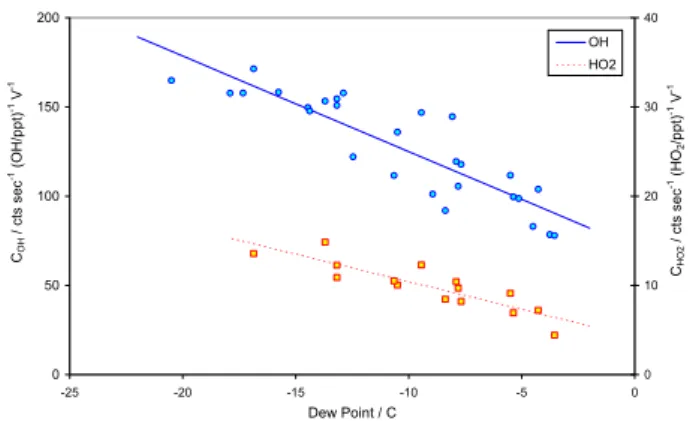
to show a stronger dependence upon humidity than can be accounted for by quenching alone, in a manner dependent upon the precise sampling geometry (nozzle diameter, shap-ing; cell design) employed (Creasey et al., 1997). During the CHABLIS campaign, ambient humidity varied between 0.11% and 0.65% (dew points of –19.4 to +0.4◦C respec-tively). Calibrations were therefore performed as a func-tion of humidity. Calibrafunc-tions at a range of water levels were performed every 3 days on average (11 times in total over the 39 days of measurements), and all calibration data were averaged to determine a mean (humidity dependent) in-strument sensitivity for the campaign, which was applied to all the measured data. Figure 1 shows the humidity depen-dence of the determined calibration constants C for OH and HO2. Fewer HO2calibrations were performed due to a
lim-ited supply of CO. Under the median conditions of 0.4 % absolute humidity (dew point –5.2◦C), the instrument sensi-tivity was 17 counts s−1mW−1ppt−1for OH and 1.2 counts s−1mW−1ppt−1for HO2, corresponding to typical detection
limits of 4.8×10⁻³and 0.068 ppt (ca. 1.3×10⁵and 1.8×10⁶ molecules cm−3) respectively, in (just under) 5 min. The
difference in OH and HO2sensitivity reflects the low
con-version efficiency achieved under the configuration (nozzle diameter; NO injector arrangement; NO flow) used during CHABLIS.
2 0 50 100 150 200 -25 -20 -15 -10 -5 0 Dew Point / C CO H / ct s se c -1 (O H /p p t) -1 V -1 0 10 20 30 40 CH O 2 / c ts se c -1 (H O2 /p p t) -1 V -1 OH HO2
Fig. 1. Calibration constants for OH (blue circles) and HO2(red squares) measured during the campaign, as a function of humidity. Lines indicate linear regressions used to analyse the ambient HOx data. The data are given in terms of laser power in the fluorescence cell, measured via UV photodiode, and can be converted approxi-mately into units of counts s−1(HOx/ppt)−1mW−1by dividing by 6. -1 0 1 2 3 4 5 3 9 15 21 27 33 39 Julian Day, 2005 O H / 1 0 6 cm -3 -3 -2 -1 0 1 2 3 H O2 / p p t o r j(O 1D )/ 5 x1 0 -4 s -1 OH HO2 j(O1D)
Fig. 2. Time series of OH (molecule cm−3; blue) and HO2(ppt, red, upper panel) data for the campaign, together with j (O1D) (s−1; black line, upper panel).
The overall uncertainty in the HOxlevels determined via
Eq. (2), and hence the instrument calibration, can be calcu-lated from the uncertainty in the individual factors. System-atic uncertainties in the values of the water and oxygen cross sections, the profile factor and the accuracy of the ozone analyser and dew-point hygrometer give an uncertainty of 22% when combined in quadrature. To this must be added the precision in the ozone and water measurements, which largely accounts for the scatter apparent in Fig. 1, and which we estimate to be 15%, giving a combined uncertainty for this campaign of 27%. As in practice the average of multiple calibrations was used to analyse the HOx data (i.e. the
re-gression lines shown in Fig. 1), this value may over estimate the total uncertainty, although naturally only known sources of error are taken into account. Interference tests were per-formed during the campaign, in which C3F6 was added to
the calibration flow, resulting in the removal of all OH
radi-cals (Dubey et al., 1996); the instrument signal fell to back-ground levels. No signal was observable when the NO flow was turned on (during calibration, with the mercury lamp off, i.e. in the absence of any OH or HO2radicals),
indicat-ing that any HO2artefact (arising from, for example, HONO
and/or HNO3formation in the NO supply line, both of which
may photolyse in the laser pulse to form OH) was below de-tectable levels. The NO titration flow was replaced with N2,
and turned on/off during normal calibration, with no change in the detected OH signal, indicating that flow disturbance in the cell arising from the gas injection was negligible.
5 OH and HO2observations
Figure 2 shows the entire OH and HO2dataset obtained at
Halley, together with j (O1D) as determined by a spectral ra-diometer. HOx data were recorded on 37 days between 3
January and 10 February 2005, including a near-unbroken 5-week spell from 11 January – the instrument was shut down as blizzard conditions prevented access to the measurement site over the 8–10 January period. The campaign yielded slightly over 4000 10-min averaged OH and HO2data points.
As Fig. 2 shows, OH and HO2followed a diurnal profile
very closely coupled to the variation in photolysis rates. HOx
levels were above zero even at their lowest levels – as Halley lies within the Antarctic circle, 24 h daylight is present dur-ing January and early February (maximum solar zenith angle of 82◦–89◦; 11 January–13 February – for comparison, the minimum values j (O1D) and j (NO2) “at night” were 2.6 %
and 11.4 % of their maximum values, on average over the measurement period). A seasonal cycle is clearly visible in the j (O1D) and OH data, with maximum and minimum val-ues decreasing towards the end of the measurement period as solar zenith angles increased. The trend is less clear in HO2, reflecting both the more complex HO2production and
removal chemistry, and the natural buffering of HO2levels
which results from self-reaction accounting for a significant fraction of their removal.
The OH and HO2levels were observed to respond to
lo-cal (base generator exhaust) pollution events: Figure 3 shows the response of HOxto an NO spike experienced at the
mea-surement location, as the local wind direction veered from westerly to easterly in a clockwise manner (through North), bringing exhaust from the base generators, containing NOx,
over the measurement site at approximately 9 am on 30 Jan-uary. OH levels rise and HO2levels fall in response to the
NOxperturbation. Note the data shown are 10-minute
aver-ages, thus the fine structure in the NO and HOxvariation is
obscured. The remainder of the day shows a diurnal cycle in radical levels in response to solar radiation.
No obvious correlations with local meteorology were ob-served for the HOxlevels other than the variations with
pho-tolysis rates, temperature, humidity etc. which would be ex-pected. In particular, no dependence upon wind direction
-360 -180 0 180 360 00:00 06:00 12:00 18:00 00:00 Time / UT W in d D ire c ti o n & N O / 1 0 p p t 0 0.5 1 1.5 2 2.5 3 3.5 O H / 1 0 6 cm -3 & H O2 / p p t NO Wind Dir OH HO2
Fig. 3. HOxperturbation due to base pollution event of 30 January. Time series of OH (red circles, 106molecule cm−3) and HO2(blue circles, ppt) (lower panel), together with NO (black line, ppt/10) and local wind direction (pink line) (upper panel).
(within the clean air sector) or wind speed was observed, which contrasts with the elevated levels of OH reported at high wind speeds for Summit, Greenland (Sjostedt et al., 2005). On several occasions, local radiation fog was ob-served to form, usually in a layer a few metres thick encom-passing the inlet height for the LIF system. During these events, radical levels fell below the detection limit.
The raw data were filtered to exclude air from the base air sector (local wind directions from 290◦to 345◦) or
dur-ing very low wind speeds (<1 ms−1), when recycling of air
from the CASLab exhaust could have occurred. Of the re-maining measurements (90.0% of the total), the mean OH concentration was 3.9×105cm−3, with mean maximum and minimum values of 7.9×105cm−3and 8.2×104cm−3 (max-imum/minimum values of the mean level, for each hour of the day, averaged over the whole campaign). The corre-sponding mean HO2mixing ratio was 0.76 ppt, with
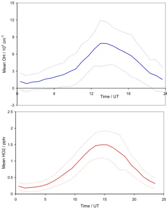
max-imum and minmax-imum levels of 1.50 and 0.18 ppt respectively. Figure 4 shows the mean and single standard deviation for all (filtered) values of OH and HO2, in hourly bins.
6 Empirical relationship to photolysis rates
Photolysis of various precursor species ultimately determines the rate of production of HOx and, as a consequence of
the relatively short and constant OH and HO2 lifetime, is
strongly related to HOx concentrations. Observed OH and
HO2 levels can therefore frequently be expressed as
rela-tively simple functions of photolysis rates, which can pro-vide both a convenient parameterisation for the HOx levels
in a particular environment, and an insight into the chemical processes controlling their abundance.
The dependence of OH levels upon the rate of production of electronically excited oxygen atoms, j (O1D), depends upon the chemical environment: In the absence of NOxand
-3 0 3 6 9 12 15 0 6 12 18 24 Time / UT Me a n O H / 1 0 5 cm -3 0 0.5 1 1.5 2 2.5 0 5 10 15 20 25 Time / UT Me a n H O 2 / p p tv
Fig. 4. Hourly mean values of (a) OH and (b) HO2observed during the campaign, together with ±1 standard deviation values. Data filtered to exclude base pollution as described in the text.
halogen species, primary production via reactions R1 and R2 is expected to dominate, and OH is expected to show an ap-proximately linear relationship with j (O1D), with some de-viation due to HO2+ O3and H2O2photolysis. At higher NO
levels, or in the presence of halogen oxides (XO), processes such as the HO2+ NO reaction, HO2+ XO and HONO
pho-tolysis are of increasing importance and the relationship be-tween OH and j (O1D) becomes more complex. In their anal-ysis of OH data acquired at a rural site in Germany, Ehhalt and Rohrer (2000) have shown that for a particular NOxlevel
the dependence of OH upon j (O1D) can be better described by an expression of the form OH = a×j (O1D)b, where the non-unity exponential parameter incorporates the influences of (e.g.) j (NO2) and j (HONO) upon OH production, via
HO2+ NO and HONO photolysis respectively. Subsequently
the addition of an intercept, allowing for non-photolytic rad-ical sources (e.g. NO3 chemistry or alkene ozonolysis) has
been shown to improve the correlations in some environ-ments (Smith et al., 2006). HO2can also be parameterised
in terms of j (O1D); in the absence of NOx(or XO species),
peroxy radical levels are expected to be approximately lin-early related to j (O1D)1/2 (Penkett et al., 1997). With in-creasing NOx(or XO), radical cycling from RO2to HO2and
HO2to OH becomes more significant, and the exponent may
2 -5 0 5 10 15 20 25 30 0 1 2 3 4 5 6 j(O1 D) / 10-5 s-1 O H / 1 0 5 cm -3 -8 -6 -4 -2 0 2 4 6 H O2 / 1 0 7 cm -3 OH HO2
Fig. 5. Variation of clean-air sector OH and HO2data with j (O1D), together with fits to Eq. (3).
At Halley in summer, while NO levels are low (relative to the moderately polluted sites considered by Ehhalt and Rohrer), the halogen oxides make a significant contribution to OH production via photolysis of HOI and/or HOBr, and HCHO photolysis contributes significantly to the production of HO2 (see below). We therefore expect some deviation
from a linear dependence of OH upon j (O1D). The depen-dence of the OH and HO2 observations upon j (O1D) was
investigated by fitting Eq. (3), below, to each dataset:
X = a × {j (O1D)/10−5s−1}b+c (3) where X = OH/105molecule cm−3or X = HO2/107molecule
cm−3. The resulting values of a, b and c are summarised in Table 2, together with comparisons to the equivalent pa-rameters reported for other environments, and are shown on Fig. 5.
7 OH production, removal and steady state analysis
In this section the observed OH levels are compared with val-ues predicted using simple steady-state calculations. These calculations neglect (for example) reaction of OH and HO2
with intermediates in the degradation of VOCs, and produc-tion of HOx through the photolysis of carbonyl
intermedi-ates; nonetheless they serve to indicate the key features of the atmospheric chemistry. A full model simulation, includ-ing integrated HOx-NOx-XO chemistry, is the subject of a
separate manuscript (Bloss et al., 20071).
OH production
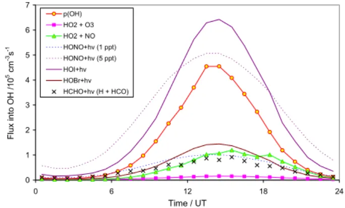
Figure 6 shows the mean OH production rates over a diurnal period, obtained from an average of all filtered data over the measurement period, for ozone photolysis, reaction of HO2
with O3and with NO, and photolysis of HONO at constant
levels of 1 and 5 ppt. Also shown for comparison is the rate of production of HO2from the H + HCO channel of
formalde-hyde photolysis. Kinetic and photochemical parameters from
0 1 2 3 4 5 6 7 0 6 12 18 24 Time / UT F lu x i n to O H / 1 0 5 cm -3s -1 p(OH) HO2 + O3 HO2 + NO HONO+hv (1 ppt) HONO+hv (5 ppt) HOI+hv HOBr+hv HCHO+hv (H + HCO)
Fig. 6. Calculated mean diurnal variation of principal OH
produc-tion mechanisms over the measurement period; see text for details. p(OH) indicates primary OH production through ozone photolysis.
Sander et al. (2006) were used. OH production from hydro-gen peroxide formation is not shown (for clarity) – the mean level of H2O2observed during the measurement period was
79 ppt (Walker et al., 2006), which would give rise to pho-tolytic OH production equivalent to approximately half that shown for 1 ppt of HONO on Fig. 6.
The DOAS system described earlier detected the halogen oxides IO and BrO at Halley during the CHABLIS cam-paign (Saiz-Lopez et al., 2007a). During the summertime period (January/February 2005), IO was observed to follow a diurnal profile with average mixing ratios ranging from ap-proximately 0.7 ppt to 5.5 ppt. BrO levels were comparable. The halogen monoxide radicals were detected in most DOAS spectra (of the appropriate wavelength region) indicating that they are likely to have been present most of the time, and to significantly affect the boundary layer radical chemistry. IO and BrO will affect HOx levels through a number of
pro-cesses, most significantly (from the perspective of perform-ing steady-state OH calculations) by convertperform-ing HO2to OH
via formation of HOI and HOBr, which may then undergo photolysis, heterogeneous loss or reaction with OH :
HO2+XO → HOX + O2 (R12)
HOX + hv → OH + X (R13)
HOX + aerosol → loss (R14)
HOX + OH → H2O + XO (R15)
The contribution of halogen-mediated HO2→OH conversion
can be approximately calculated by assuming HOI / HOBr are in steady state defined by reactions R12-R14:
[HOX]ss=k12[HO2][XO]/(j13+k14) (4)
Aerosol loss of HOI and HOBr is likely to be signifi-cant (Bloss et al., 2005); however the reaction probabil-ity is poorly known and unfortunately no aerosol surface
-0.5 0 0.5 1 1.5 2 2.5 36 37 38 39 40 41 Julian Day O H / 1 0 6 cm -3 [OH] Scenario 1 Scenario 2 Scenario 3
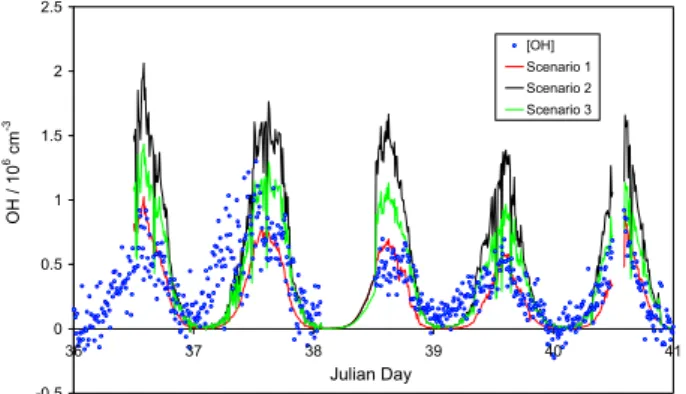
Fig. 7. Measured OH concentrations for 6–10 February 2005, days
36–40, together with calculated steady-state levels; see text for de-tails.
area measurements were available during CHABLIS. We have calculated the contribution of HOI photolysis to OH production, via Eq. (4), assuming an aerosol surface area of 1×10⁻⁷cm2cm−3(Davison et al., 1996) and a reaction probability of 0.2 for both HOBr and HOI. (k’uptake
calcu-lated using the free molecular approximation). HOI photoly-sis is approximately 200 times faster than heterogeneous loss under these assumptions at midday, and about 5 times faster at the maximum solar zenith angle; thus the impact of er-rors in the aerosol parameters assumed upon calculated OH is small for much of the day. Reaction of HOX with OH can be neglected (the relative rates of Reactions R13 and R15 at noon under the conditions at Halley were 247:1 for HOI). The resulting OH production rates are also shown on Fig. 6.
OH removal
Considering the species measured during CHABLIS, OH re-moval was dominated by reaction with CO (54.2%), CH4
(33.0%), and H2 (8.9%), with smaller contributions from
DMS, alkenes (iso-butene, propene, ethene), H2O2, NO2and
ethane (all 0.03–1%). Methanol was not measured, but antic-ipated levels (200 ppt, Jacob et al., 2005) would correspond to a 0.4% contribution to OH loss. Of the measured species, OH removal is clearly dominated by CO and CH4. The
im-pact of methane is reduced compared with boundary layer locations at lower latitudes due to the strong temperature de-pendence of the OH + CH4 rate coefficient, E/R = 1775 K
(Sander et al., 2006). The measured sinks correspond to a mean OH (e−1) lifetime of 2.1 seconds during the
measure-ment period.
No measurements of oxygenated VOCs (other than formaldehyde) were available during CHABLIS. Higher aldehydes have been observed in the Arctic boundary layer (Boudries et al., 2002), and in conjunction with firn air ob-servations suggest a net snowpack source to the overlying atmosphere (Guimbaud et al., 2002), potentially originating
Table 2. Parameters for empirical fits of OH and HO2 levels to
j (O1D) via Eq. (3).
Fitting Eq. (3) to all OH data
Fit a b c r2
1 Linear 2.22±0.02 1 (fixed) 0 (fixed) 0.38
2 Power 3.89±0.06 0.51±0.01 0 (fixed) 0.46
3 Power/Intercept 2.52±0.16 0.74±0.04 1.06±0.12 0.48
Calculated OH 4.66±0.09 0.63±0.02 0±0.1 –
Fitting Eq. (3) to all HO2data
4 Power 1.61±0.01 0.40±0.01 0 (fixed) 0.60
Notes: Uncertainties are ±1 s.d. Calculated OH refers to the fit obtained from OH levels calculated under scenario 3.
Literature values for OH and HO2–j (O1D) parameterisations
a b c
OH
Brauers et al. (2001)
ALBATROSS, Tropical Atlantic
13.7 1 (fixed) 0 (fixed) Holland et al. (2003)
BERLIOZ – Rural Germany
201 1 (fixed)1 0 (fixed)1 Smith et al. (2006)
NAMBLEX, Mace Head, Ireland
14.7 0.84±0.05 4.4
Rohrer and Berresheim (2006) Hohenpeissenberg Observatory
24 1 1.3
Berresheim et al. (2003) MINOS (Coastal Crete)
72 0.68 1
HO2
Holland et al. (2003) BERLIOZ (low NO)
201 1 (fixed)1 0 (fixed)1
Notes: Uncertainties are ±1 s.d. Values from literature sources have been adjusted to be in terms of OH/105, rather than 106, for consis-tency. 1: Estimated from figures in manuscript (values not given).
from the organic matter within snowpack. Laboratory exper-iments have shown similar production of acetaldehyde from South Pole snow (Grannas et al., 2004), thus a similar mech-anism might be expected to operate in other, related envi-ronments, i.e. at Halley. Acetaldehyde and other carbonyl species would affect the local radical chemistry, both through photolysis leading to radical production, and through direct reaction with OH providing an additional OH sink. For ex-ample, if acetaldehyde was present at the levels observed in the Arctic (29–459 ppt during the 24-h daylight period – Boudries et al., 2002), the total OH sink would be increased by between 3 and 48%, giving a considerable reduction in the OH lifetime.
2
Steady-state OH levels
Figure 7 shows a 5-day period (Julian days 36–40) of mea-sured OH concentrations, and steady-state OH levels calcu-lated according to the three scenarios listed below, described in more detail in the following section:
1. Production from O3photolysis and the reactions of HO2
with NO and O3
Loss due to reaction with all measured sinks
2. As 1 but with additional OH production due to HOI pho-tolysis
3. As 2 but with an additional OH sink: Reaction with ac-etaldehyde
Scenario 1 reflects the conventional tropospheric chemistry which might be expected for a remote location.
Scenario 2 allows a semi-quantitative investigation of the impact of the halogen oxides, IO and BrO, upon OH levels. IO and BrO absorb in different wavelength regions, thus no simultaneous observations of both halogen monoxides were possible from the DOAS. The IO dataset is the more exten-sive of the two during the HOxmeasurement period (more
time was spent measuring IO than BrO), consequently the IO data has been used here as a proxy for the total impact of XO (IO and BrO) upon HOx. The IO dataset is itself limited
compared with the OH observations, consequently IO levels were calculated from a purely empirical relationship between the DOAS IO observations over the summer period and the corresponding measurements of j (NO2), which were found
to be highly correlated:
IO/ppt=(j (NO2)/s × 280) + 0.7 (5)
HOI was assumed to be in steady state, defined as described by Eq. (4).
Scenario 3 considers the likely possibility that further, un-measured VOCs are present and provide additional OH sinks. An additional OH sink was added to the calculation, equal in magnitude to 167 ppt of acetaldehyde (on average), varying diurnally with j (NO2) – selected to replicate the CH3CHO
observations reported in the Arctic (Boudries et al., 2002). In addition to scenarios 1–3, further production of OH might also be expected to result from HONO photolysis; this pos-sibility is examined in the Discussion section.
8 Discussion
The OH levels measured in coastal Antarctica during the CHABLIS campaign are reasonably consistent with those observed at Palmer Station on the Antarctic Peninsula (Jef-ferson et al., 1998), but are considerably lower than those observed at South Pole (Mauldin et al., 2001, 2004). The mean HO2level observed at Halley is also rather lower than
HO2+ RO2levels observed at South Pole during ISCAT2000
(Mauldin et al., 2004), by a factor of 3–4. The Halley HO2
levels are however higher than those observed at Summit, Greenland (by a factor of 3 for the summer campaign) – (Sjostedt et al., 2005).
The contrast between the HOx levels at Halley and the
higher levels at South Pole can be explained largely by the effect of the low mixed layer height at South Pole ampli-fying the effect of snowpack emissions of NOx (Davis et
al., 2004), HCHO and H2O2(Chen et al., 2004) resulting in
NO levels averaging 100–200 ppt. At such levels, NO domi-nates HOxcycling and OH levels, and the effects of halogen
species upon HOxlevels would be small; moreover
bound-ary layer halogen levels are expected to be negligible at the pole. Daytime boundary layer heights of 100 m have been inferred for Halley during the CHABLIS campaign (Ander-son, 2006). It is also worth noting that the South Pole site re-ceived near-uniform sunlight around the solstice, while Hal-ley experiences a significant diurnal cycle (Fig. 2). Observa-tions of nitrous acid, HONO, were also reported from South Pole during the ISCAT2000 campaign (Dibb et al., 2004), with mixing ratios of around 30 ppt measured using a mist chamber/ion chromatography technique. HONO photolyses rapidly in the boundary layer, with a lifetime of a few min-utes (250 s at noon during CHABLIS on average), thus ppt levels of HONO would make a large contribution to the HOx
budget. Modelling studies were unable to reconcile the HOx
and NOxlevels observed at South Pole with the HONO
ob-servations (Chen et al., 2004). Subsequently, HONO mea-surements were performed at South Pole during the Decem-ber 2003/January 2004, using both mist chamDecem-ber/ion chro-matography and LIF approaches. The LIF system detected HONO at levels of around 6 ppt, sufficient to form a major source of HOx, but lower than the concurrent mist chamber
observations by a factor of 7 (Liao et al., 2006).
HONO measurements were also performed during CHABLIS: measurements were performed by stripping to the aqueous phase in a glass coil chamber, followed by a complexation/diazotization reaction to produce an azo dye detectable by absorption spectroscopy (Clemitshaw, 2004). The mean HONO level observed during the HOx
measure-ment period at Halley was 7 ppt (Clemitshaw, 2006 and per-sonal communication). At such levels, HONO photolysis would dominate the HOxbudget – Fig. 6 shows the OH
pro-duction rates which would result from constant levels of 1 and 5 ppt HONO. This would lead to the HOx steady-state
levels far exceeding the observations, even in the hypothe-sised presence of additional oxygenated organic species con-tributing to the total OH sink. The NO production resulting from HONO photolysis would also lead to calculated NOx
levels far greater than those observed – The mean NOxlevel
at Halley during the HOx measurement period was 15 ppt
(Bauguitte et al., 2005) with a lifetime of approximately 6 h (consistent with heterogeneous hydrolysis of halogen ni-trates). This can be compared with the HONO photolytic
lifetime of approximately 4–10 min, indicating that a few ppt of HONO would be expected to produce much higher NOx levels. In common with the earlier South Pole
stud-ies, we cannot currently reconcile the HOxand NOx
observa-tions with the observed HONO data, without invoking a large unidentified additional HOxand NOxsink. A positive
arte-fact in the HONO data could explain this discrepancy: The technique in practice detects total soluble nitrite, thus con-tributions from aerosol, from peroxynitric acid, or from the halogen nitrite species INO2and BrNO2, could contribute to
the measured signal - however the concentrations of the latter are calculated to be a fraction of a ppt under the conditions prevalent at Halley.
The presence of significant levels of halogen activity was confirmed during CHABLIS by the DOAS observations of IO and BrO (Saiz-Lopez et al., 2007a). Due to the nature of the DOAS system, the halogen observations were less fre-quent than the HOx data during the summer period;
how-ever IO was detected during how-every attempted observation, at levels which were well described by Eq. (5). It is therefore likely that both iodine and bromine species were present in the boundary layer at Halley throughout the summer cam-paign, with a number of impacts upon the chemical com-position: As described above, the halogens act to drive the radical cycling from organic peroxy radicals to HO2to OH,
with concomitant ozone destruction due to the reformation of halogen atoms. Additional ozone destruction will also result from the halogen oxide cross- and self-reactions, IO + IO, IO + BrO and BrO + BrO. Further, the halogens will change the NOx partitioning (through the IO + NO and BrO + NO
reactions), and provide an additional NOxsink, through
for-mation and the subsequent deposition or heterogeneous loss of halogen nitrates. (The calculated halogen nitrate sink re-duces the NOxlifetime to around 6 h, insufficient to reconcile
NOx levels with the NO production that would result from
photolysis of the observed levels of HONO – Bauguitte et al., 2006). Reaction with IO and with BrO forms the domi-nant sink for HO2 and source of OH. Production of HI and
HBr are likely to add to the HOxsink. Peroxy radical levels
may be increased due to elevated OH levels and reductions in HO2, but this effect will be offset by the RO2+ XO reactions,
depending upon the kinetics employed. The full impacts of the halogen species are considered in the detailed box and 1-dimensional model studies reported elsewhere (Bloss et al., 20071; Saiz-Lopez et al., 2007b).
The observed levels of OH were reproduced reasonably well by steady-state OH levels calculated under scenario 1 (Fig. 7), with a calculated:observed ratio of 0.67, reflecting conventional remote tropospheric chemistry disregarding the effect of halogens and HONO, are in good agreement with the observations. However, HOBr and (particularly) HOI photolysis will lead to additional OH production, and to a significant over-prediction of the measured OH levels (sce-nario 2, mean calculated:observed ratio = 1.64). While the IO present on a given day may well have been less than that
assumed through Eq. (5), scenario 2 neglects the additional HO2to OH conversions anticipated through HOBr formation
and photolysis, i.e. the impact of BrO. Observed BrO levels were comparable with those of IO (Saiz-Lopez et al., 2007a), on which basis the contribution of HOBr photolysis to OH formation is anticipated to be approximately 4 times smaller than that of HOI (due to the lower BrO+HO2rate constant
and HOBr cross sections). Addition of a further OH sink would improve the agreement: The hydrocarbon measure-ments during CHABLIS (C2-C6 alkanes, alkenes and aro-matics) notably excluded oxygenated hydrocarbons (other than HCHO), which react reasonably rapidly with OH and have been shown to form a significant portion of the total rad-ical sink in the marine boundary layer (Lewis et al., 2005). Acetaldehyde, acetone and other oxygenated VOCs were ob-served during ALERT in the Arctic (Boudries et al., 2002) indicating that such compounds can reach appreciable con-centrations in the polar boundary layer environment; whether such levels are also found in the Antarctic, considerably fur-ther removed from anthropogenic emission sources, is less certain, although we note that studies have reported com-parable total organic carbon content in snow samples from South Pole, Summit (Greenland) and Alert (Grannas et al., 2004). Inclusion of an additional OH sink, equal in magni-tude to that which would result from acetaldehyde present at the levels observed in the Arctic boundary layer, largely re-stores agreement between calculated and observed OH levels (scenario 3, calculated:observed ratio = 1.27).
Figures 6 and 7 show that the halogen oxides will domi-nate the radical cycling, compared with NOx. The
environ-ment at Halley is thus one in which rapid radical cycling oc-curs, with a large chain length, but driven by XO rather than NO, and with associated ozone destruction rather than ozone production. This is in contrast with the situation in much of the troposphere, where minimal radical cycling, short chain lengths and very low NOxlevels are associated with
(pho-tolytic) ozone loss, and longer chain lengths are associated with elevated NOxand ozone production.
The HO2:OH ratio at Halley is 49.2 (mean local solar noon
value), with a median value from all (filtered) HOxdata of
37.4. These values can be compared with ratios of 44–104 observed in the Southern Ocean boundary layer in Tasmania (Creasey et al., 2003), 76 in the Western Pacific (Kanaya et al., 2001) and 90-137 during in the pacific free troposphere (Tan et al., 2001). Conventional tropospheric chemistry pre-dicts that under clean conditions (low NO), the ratio should increase as radical levels fall (due to the non-linearity in HO2
loss through self-reaction), and should decrease as NO lev-els increase (due to HO2to OH conversion); upon this basis
the observed HO2:OH ratio might be expected to be higher
than the other determinations listed above (clean conditions; low radical levels). However in the case of the Halley data, radical cycling is affected by the halogen species – the low HO2:OH ratio for Halley, under low NOxconditions, is
2
with IO and BrO. The low values of the HO2:OH ratio,
which is a particularly robust measurement product as many of the instrumental and calibration factors cancel out, fur-ther demonstrates the importance of halogen-HOxcoupling
in this environment.
OH and HO2vs. j (O1D) power dependencies
The OH and HO2 data are reasonably well described by
Eq. (3) in Fig. 5, reflecting the fact that the main processes dominating OH and HO2concentrations (photolysis of O3,
HCHO, H2O2; NOxlevels; XO levels) exhibit a strong and
similar dependence upon solar irradiation. The OH data are best described by the full version (3) of Eq. (3). The positive intercept may reflect a contribution from radical production through photolysis routes with a broader SZA dependence than j (O1D) - for example HCHO or HONO. That the ex-ponent b is less than unity is probably related to the role of halogen chemistry in driving the HOxcycling, having a
qual-itatively similar effect to NOxand reducing the direct
depen-dence of OH upon j (O1D). The HO2data is well-described
by the fit shown – addition of the intercept parameter (c) gave no significant improvement. The parameters may be compared with those obtained for measurements performed elsewhere which are also given in Table 2. The much larger OH concentrations observed in mid-latitudes are reflected in the higher value of the a coefficient, by a factor of up to 35. The similarity in the exponent b, 0.84 (Mace Head) and 0.68 (Crete) vs. 0.74 (Halley) indicates that the processes modify-ing the radicals’ response to the sunlight levels, such as re-sponse to long- and short-wavelength components, are sim-ilar – possibly reflecting NOxresponse at Crete, combined
NOx/halogen impacts at Mace Head, and halogen impacts at
Halley. The higher value for parameter c, which indicates non-photolytic radical production, probably reflects the role of ozone-alkene and NO3initiated reactions at Mace Head,
which would be much less significant at Halley (low O3;
low VOC levels; permanent (long-wavelength) illumination (summer) photolysing NO3) – although a lower value than
that recorded for Hohenpeissenberg might therefore also be expected; it is not clear why this is not the case. The ex-pressions derived to relate the OH and HO2levels to j (O1D)
may be used to roughly estimate the seasonal levels of OH and HO2, from variations in actinic flux (assuming the
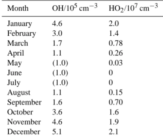
sum-mertime conditions and composition are typical of the rest of the year). Such a calculation is shown in Table 3 – these val-ues were determined using the radiative transfer model TUV (Madronich and Flocke, 1998) to calculate the 24-hour aver-age clear-sky j (O1D) level at the mid-point of each calendar month, scaling these values by comparing the January result to the actual, observed j (O1D) value and applying Eq. (3) to determine the OH/HO2level. Ozone columns were monthly
averages over the period 1999-2004 for Halley. Such a cal-culation makes a number of assumptions, including that the
Table 3. Monthly mean OH and HO2concentrations inferred from scaled calculated solar actinic flux as described in the text.
Month OH/105cm−3 HO2/107cm−3 January 4.6 2.0 February 3.0 1.4 March 1.7 0.78 April 1.1 0.26 May (1.0) 0.03 June (1.0) 0 July (1.0) 0 August 1.1 0.15 September 1.6 0.70 October 3.6 1.6 November 4.6 1.9 December 5.1 2.1
summer chemistry is representative of the rest of the year, that chemical processes dominating the radical levels are lin-early dependent upon j (O1D), and that the solar attenuation (cloudiness / weather) during January 2005 was typical of the rest of the year, but provide an indication of the annual HOx levels in this environment. This approach produces
mid-winter values of OH (May–July) which are likely to be overestimates (arising from the intercept parameter (c) in Eq. (3)), shown in parentheses in the table. The resulting an-nual mean OH concentration in the coastal Antarctic bound-ary layer is found to be 2.4×10⁵molec−1 cm3. This value is lower than the global tropospheric mean OH concentration of (9.8±1.6) ×105cm−3 (Bloss et al., 2005b), as expected given the low (annual average) light levels, absolute humidity etc. The annual trend in OH levels shown in Table 3 mirrors the seasonal variation in ethane and propane levels observed by GC measurements during the year-long CHABLIS obser-vations (Read et al., 2007). The low winter/early spring val-ues for OH (August/September) support the inference drawn by Read et al. (2007) that halogen chemistry (Cl and/or Br reactions) was responsible for shorter timescale variations in hydrocarbon ratios.
9 Conclusions
OH and HO2 radicals were measured at Halley, Antarctica
during January and February 2005, with mean radical levels of 3.9×10⁵ molecule cm−3 for OH, and 0.76 ppt for HO2.
Typical maximum (local noontime) levels were 7.9×10⁵ molecule cm−3 and 1.50 ppt respectively. These levels are consistent with earlier measurements of OH on the Antarc-tic Peninsula, but lower than recent observations from South Pole and Summit, Greenland. The main sources of HOxwere
photolysis of O3and HCHO, with potentially important but
Of the measured OH sinks, reaction with CO and CH4
dom-inated, giving a total OH lifetime of approximately 2 sec-onds; however the observed OH levels together with calcu-lated HO2to OH conversion fluxes indicated that additional
co-reactants were likely to have been present.
Elevated levels of NOx resulting from snowpack
photo-chemistry contributed to HOxcycling and enhanced levels of
OH, however the halogen oxides IO and BrO dominated the CH3O2 – HO2 – OH conversion in this environment, with
associated ozone destruction. The quantitative impact of this chemistry depends upon the details of the XO + CH3O2
re-actions and magnitude of the aerosol sink for HOX, which are poorly constrained. HONO levels of several ppt were measured during CHABLIS, indicating a substantial addi-tional HOxand NOxsource, which we are currently unable
to reconcile with the radical observations. Considering the enhanced HO2to OH conversion in the presence of the
halo-gen species, the observed OH levels indicate that substan-tial unmeasured OH sinks are present. Data from the Arctic suggest that these may be higher oxygenated VOCs such as acetaldehyde, although the halogen halides HI and HBr are alternative candidates.
The fast photochemistry and hence oxidising environ-ment of the boundary layer in coastal Antarctica is a com-plex regime affected by NOx, VOC and halogen
chem-istry, rather than a quiescent regime of low HOxproduction
through ozone photolysis coupled with straightforward re-moval through reaction with CO and CH4. This being the
case, extrapolating from the local atmospheric chemical en-vironment, as might be determined from analyses of air from firn and ice cores collected in polar regions, to the prevailing free tropospheric chemical composition may be difficult.
Acknowledgements. We wish to thank Z. Fleming, G. Mills,
K. Read and A. Saiz-Lopez for their help and contributions to the CHABLIS project, in Antarctica and beyond. The logistic assistance and support from the staff of the British Antarctic Survey is also gratefully acknowledged. We also thank T. Ingham, C. Floquet and S. Smith in Leeds, who allowed us the use of their equipment in support of the campaign. CHABLIS was funded by the Natural Environment Research Council through the Antarctic Funding Initiative, ref. NER/G/S/2001/00558.
Edited by: W. T. Sturges
References
Anderson, P. S.: Behaviour of tracer diffusion in simple atmo-spheric boundary layer models, Atmos. Chem. Phys. Discuss. 6, 13 111–13 138, 2006.
Aschmutat, U., Hessling, M., Holland, F. and Hofzumahaus, A.: A tuneable source of hydroxyl (OH) and hydroperoxy (HO2) radi-cals: In the range between 106and 109cm−3, Physico-Chemical Behaviour of Atmospheric Pollutants, edited by: Angeletti, G. and Restelli, C., Proc. EUR 15609, 811–816, 1994.
Bauguitte, S. J.-B., Bloss, W. J., Clemitshaw, K. C., Evans, M. J., Jones, A. E., Lee, J. D., Mills, G., Saiz-Lopez, A., Salmon, R. A., Roscoe, H. K., and Wolff, E. W.: An overview of year-round NOx measurements during the CHABLIS campaign: can sources and sinks estimates unravel observed diurnal cycles?, Geophys. Res. Abstr., 8, 09054, 2006.
Berresheim, H., Plass-D¨ulmer, C., Elste, T., Mihalopoulos, N., and Rohrer, F.: OH in the coastal boundary layer of Crete during MINOS: Measurements and relationship with ozone photolysis, Atmos. Chem. Phys., 3, 639–649, 2003,
http://www.atmos-chem-phys.net/3/639/2003/.
Bloss, W. J., Gravestock, T. J., Heard, D. E., Ingham, T., Johnson, G. P., and Lee, J. D.: Application of a compact all-solid-state laser system to the in situ detection of atmospheric OH, HO2, NO and IO by laser-induced fluorescence, J. Environ. Monit. 5, 21–28, 2003.
Bloss, W. J., Lee, J. D., Johnson, G. P., Sommariva, R., Heard, D. E., Saiz-Lopez, A., Plane, J. M. C., McFiggans, G., Coe, H., Flynn, M., Williams, P., Rickard, A. R., and Fleming, Z. L.: Impact of halogen monoxide chemistry upon boundary layer OH and HO2 concentrations at a coastal site, Geophys. Res. Lett., 32, L06814, doi:10.1029/2004GL022084, 2005a.
Bloss, W. J., Evans, M. J., Lee, J. D., Sommariva, R., Heard, D. E., and Pilling, M. J.: The oxidative capacity of the troposphere: Coupling of field measurements of OH and a global chemistry transport model, Faraday Discuss.,130, 425–436, 2005b. Boudries, H., Bottenheim, J. W., Guimbaud, C., Grannas, A. M.,
Shepson, P. B., Houdier, S., Perrier, S., and Domin´e, F.: Distri-bution and trends of oxygenated hydrocarbons in the high Arctic derived from measurements in the atmospheric boundary layer and interstitial snow air during the ALERT2000 field campaign, Atmos. Environ., 36, 2573–2583, 2002.
Brauers, T., Hausmann, M., Bister, A., Kraus, A., and Dorn, H. P.: OH radicals in the boundary layer of the Atlantic Ocean 1. Mea-surements by long-path laser absorption spectroscopy, J. Geo-phys. Res., 106, 7399–7414, 2001.
Cantrell, C. A., Zimmer, A., and Tyndall, G.S.: Absorption cross sections for water vapour from 183 to 193 nm, Geophys. Res. Lett., 24, 17, 2195–2198, 1997.
Chen, G., Davis, D., Crawford, J., Nowak, J.B., Eisele, F., Mauldin III, R.L., Tanner, D., Buhr, M., Shetter, R., Lefer, B., Arimoto, R., Hogan, A., and Blake, D.: An Investigation of South Pole HOx Chemistry: Comparison of Model Results with ISCAT Ob-servations, Geophys. Res. Lett., 28, 3633–3636, 2001.
Chen, G., Davis, D., Crawford, J., Hutterli, L. M., Huey, L. G., Slusher, D., Mauldin, L., Eisele, F., Tanner, D., Dibb, J., Buhr, M., McConnell, J., Lefer, B., Shetter, R., Blake, D., Song, C. H., Lombardo, K., and Arnoldy, J.: A reassessment of HOx South Pole chemistry based on observations recorded during ISCAT 2000, Atmos. Environ., 38, 5451–5461, 2004.
Clemitshaw, K. C.: A Review of Instrumentation and Measure-ment Techniques for Ground-Based and Airborne Field Studies of Gas-Phase Tropospheric Chemistry, Critical Reviews in Envi-ronmental Science and Technology, 34, 1–108, 2004.
Clemitshaw, K. C.: Coupling between Tropospheric Photochem-istry of Nitrous Acid (HONO) and Nitric Acid (HNO3), Environ. Chem., 3, 31–34, 2006.
Creasey, D. J., Heard, D. E., and Lee, J. D.: Absorption cross-section measurements of water vapour and oxygen at 185 nm.