Technical Note: Chemistry-climate model SOCOL: version 2.0 with improved transport and chemistry/microphysics schemes

HAL Id: hal-00304244

https://hal.archives-ouvertes.fr/hal-00304244

HAL is a multi-disciplinary open access

archive for the deposit and dissemination of sci-entific research documents, whether they are pub-lished or not. The documents may come from teaching and research institutions in France or abroad, or from public or private research centers.

L’archive ouverte pluridisciplinaire HAL, est destinée au dépôt et à la diffusion de documents scientifiques de niveau recherche, publiés ou non, émanant des établissements d’enseignement et de recherche français ou étrangers, des laboratoires publics ou privés.

Technical Note: Chemistry-climate model SOCOL:

version 2.0 with improved transport and

chemistry/microphysics schemes

M. Schraner, E. Rozanov, C. Schnadt Poberaj, P. Kenzelmann, A. M. Fischer,

V. Zubov, B. P. Luo, C. R. Hoyle, T. Egorova, S. Fueglistaler, et al.

To cite this version:

M. Schraner, E. Rozanov, C. Schnadt Poberaj, P. Kenzelmann, A. M. Fischer, et al.. Technical Note: Chemistry-climate model SOCOL: version 2.0 with improved transport and chemistry/microphysics schemes. Atmospheric Chemistry and Physics Discussions, European Geosciences Union, 2008, 8 (3), pp.11103-11147. �hal-00304244�

ACPD

Full Screen / Esc

Printer-friendly Version

Interactive Discussion Atmos. Chem. Phys. Discuss., 8, 11103–11147, 2008

www.atmos-chem-phys-discuss.net/8/11103/2008/ © Author(s) 2008. This work is distributed under the Creative Commons Attribution 3.0 License.

Atmospheric Chemistry and Physics Discussions

Technical Note: Chemistry-climate model

SOCOL: version 2.0 with improved

transport and chemistry/microphysics

schemes

M. Schraner1,2, E. Rozanov1,2, C. Schnadt Poberaj1, P. Kenzelmann1,

A. M. Fischer1, V. Zubov3, B. P. Luo1, C. R. Hoyle4, T. Egorova2, S. Fueglistaler5, S. Br ¨onnimann1, W. Schmutz2, and T. Peter1

1

Institute for Atmospheric and Climate Science, ETH Z ¨urich, Switzerland

2

Physical-Meteorological Observatory/World Radiation Center, Davos, Switzerland

3

Main Geographical Observatory, St.-Petersburg, Russia

4

Department of Geosciences, University of Oslo, Norway

5

DAMTP, University of Cambridge, UK

Received: 8 April 2008 – Accepted: 7 May 2008 – Published: 9 June 2008 Correspondence to: M. Schraner ([email protected])

Published by Copernicus Publications on behalf of the European Geosciences Union.

ACPD

Full Screen / Esc

Printer-friendly Version

Interactive Discussion

Abstract

We describe version 2.0 of the chemistry-climate model (CCM) SOCOL. The new version includes fundamental changes of the transport scheme such as transport-ing all chemical species of the model individually and applytransport-ing a family-based correc-tion scheme for mass conservacorrec-tion for species of the nitrogen, chlorine and bromine

5

groups, a revised transport scheme for ozone, furthermore more detailed halogen reaction and deposition schemes, and a new cirrus parameterisation in the tropical tropopause region. By means of these changes the model manages to overcome or considerably reduce deficiencies recently identified in SOCOL version 1.1 within the CCM Validation activity of SPARC (CCMVal). In particular, as a consequence of these

10

changes, regional mass loss or accumulation artificially caused by the semi-Lagrangian transport scheme can be significantly reduced, leading to much more realistic distribu-tions of the modelled chemical species, most notably of the halogens and ozone.

1 Introduction

Projection of the global climate and the ozone layer is one of the central questions in

15

the contemporary geosciences (IPCC, 2006; WMO, 2007). The behaviour of the cli-mate system depends on the multitude of external forcings, on physical, chemical and dynamical processes in the atmosphere, and on their nonlinear interactions. Therefore, it can be properly assessed only with sophisticated chemistry-climate models (CCMs), which are able to treat the relevant processes (Eyring et al., 2007). On the other

20

hand, the nonlinearity of the system and uncertainty in the forcing scenarios require multiple long-term model ensemble runs, which are feasible only with models being computationally not too expensive. As a result, the limitations of a CCM caused by the lack of complete knowledge of nature, as well as by simplified descriptions of un-resolved processes are further aggravated by the necessity to exploit the fastest, but

25

repre-ACPD

Full Screen / Esc

Printer-friendly Version

Interactive Discussion sents a compromise between our ambition to have a perfect model based on the first

principles and the limits of possibility. To judge the success of this compromise, it is necessary to validate the models against observations. In previous years, CCMs have been extensively evaluated (e.g., Austin et al., 2003; Eyring et al., 2006). In these eval-uation studies several of the tested models displayed characteristic weaknesses and

5

deficiencies. For example, stratospheric temperature biases may affect temperature-dependent chemical reaction rates and lead to significant model-to-model variations in the simulation of polar stratospheric cloud (PSC) volumes in polar regions (e.g., Austin et al., 2003). Deficiencies in transport schemes may lead to errors in the temporal and spatial evolution of the distributions of ozone and other chemical species that react with

10

ozone (e.g., Eyring et al., 2006). Biases in chlorine and bromine-containing species, which are often related to deficiencies in transport, may strongly affect the catalytic ozone destruction, especially over Antarctica. Problems in simulating stratospheric water vapour may affect the radiative balance, the HOx-cycles and the formation of

PSCs in the models (e.g., Eyring et al., 2006).

15

The CCM SOCOL (modelling tool for studies of SOlar Climate Ozone Links) under investigation in the present paper has been developed at Physical and Meteorological Observatory/World Radiation Center (PMOD/WRC), Davos in collaboration with ETH Z ¨urich and MPI Hamburg (Egorova et al., 2005). The evaluation of different CCMs within the Chemistry-Climate Model Validation Activity for SPARC, CCMVal (Eyring et

20

al., 2006), revealed that SOCOL has serious problems in simulating the stratospheric chlorine content and water vapour. In the upper stratosphere, the mixing ratio of to-tal inorganic Cl_y simulated by the CCM SOCOL was up to 30% higher than that of the maximum total chlorine entering the stratosphere. In contrast, in the lower strato-sphere of the southern high latitudes total inorganic Clywas shown to be significantly

25

underestimated by SOCOL (1.1 ppbv at 50 hPa, 80◦S for October 1992, in contrast to 3.0 ppbv from estimates based on HALOE observations; Eyring et al. (2006), their Fig. 12). Water vapour was overestimated by 30–40% in the whole stratosphere (see Eyring et al. (2006), their Fig. 6). On the other hand, it was shown that SOCOL

ACPD

Full Screen / Esc

Printer-friendly Version

Interactive Discussion isfactorily represents the distributions of many other trace gases outside the southern

polar vortex, as well as atmospheric temperature and dynamics. Owing to SOCOL’s excellent computational efficiency and portability allowing its application for long-term ensemble runs on regular personal computers (Egorova et al., 2005), we were able to evaluate possible causes of the model deficiencies and to overcome them in a

physi-5

cally meaningful manner without dramatic and expensive redesign of the entire model. In the present paper, we illustrate a step-by-step evaluation of the problems in SOCOL and the implementation of specific changes in the transport and chemical modules leading to significantly improved model performance. We believe that our efforts will be useful for other modelling groups having similar problems with chemistry and transport

10

representation in their models.

In the following, we will refer to the original version of SOCOL described by Egorova et al. (2005) and Rozanov et al. (2005) as SOCOL vs1.0, the SOCOL version partici-pating in the CCMVal evaluation of Eyring et al. (2006) as SOCOL vs1.1, and the new version presented in this paper as SOCOL vs2.0. This paper is organized as follows.

15

Section 2 gives a model description of SOCOL vs1.1. Section 3 describes the bound-ary conditions and model set up of the simulations described in this paper. In Sect. 4, all modifications leading from SOCOL vs1.1 to SOCOL vs2.0 are described (via sub-versions termed vs1.2 to vs1.5) and the changes in relevant chemical and dynamical fields resulting from the model modifications are discussed. In Sect. 5, results from the

20

new model version SOCOL vs2.0 are compared to observations.

2 SOCOLv.1.1: model description

The CCM SOCOL is a combination of a modified version of the middle atmosphere GCM MA-ECHAM4 (Middle Atmosphere version of the “European Center/HAmburg

Model 4”) (Roeckner et al., 1996; Manzini and Bengtsson, 1996) and a modified

ver-25

sion of the CTM MEZON (Model for Evaluation of oZONe trends) (Rozanov et al., 1999, 2001; Egorova et al., 1999, 2001; Hoyle, 2005). In the original version SOCOL

ACPD

Full Screen / Esc

Printer-friendly Version

Interactive Discussion vs1.0 (Egorova et al., 2005; Rozanov et al., 2005) MA-ECHAM4 and MEZON are

in-teractively coupled by the radiative forcing induced by water vapour and ozone. For SOCOL vs1.1, this coupling was extended to include also methane, nitrous oxide, and chlorofluorocarbons (CFCs).

MA-ECHAM4 is a spectral GCM with T30 horizontal truncation resulting in a

geo-5

graphical grid spacing of about 3.75◦. In the vertical direction, the model has 39 levels in a hybrid sigma-pressure coordinate system spanning the model atmosphere from the surface to 0.01 hPa (≈80 km). A semi-implicit time stepping scheme with weak filter is used with a time step of 15 min for dynamical processes and physical process param-eterisations. Full radiative transfer calculations are performed every 2 h, but heating

10

and cooling rates are interpolated every 15 min. The radiation scheme is based on the radiation code of the European Centre of Medium-Range Weather Forecasts, ECMWF (Fouquart and Bonnel, 1980; Morcrette, 1991). In order to obtain realistic heating rates in the upper stratosphere and in the mesosphere, the absorption by O₂and O₃ in the Lyman-alpha line, Schumann-Runge bands and part of the ozone Hartley band (below

15

250 nm, which is not included in MA-ECHAM4) is taken into account in SOCOL vs1.1 (Egorova et al., 2004) using a parameterisation according to Strobel (1978). The pa-rameterisation of momentum flux deposition due to a continuous spectrum of vertically propagating gravity waves follows Hines (1997a,b), gravity wave momentum deposition is described by Doppler spread parameterisation according to Manzini et al. (1997).

20

The Doppler spread parameterisation leads to a significant improvement of the zonal winds in the mesosphere and of the semiannual oscillation of the zonal winds at the stratopause (Manzini et al., 1997).

The chemical-transport part MEZON has the same vertical and horizontal resolution as MA-ECHAM4, and the calculations are performed every 2 h. The model includes

25

41 chemical species of the oxygen, hydrogen, nitrogen, carbon, chlorine and bromine groups, which are determined by 118 gas-phase reactions, 33 photolysis reactions and 16 heterogeneous reactions in/on aqueous sulphuric acid aerosols, water ice and nitric acid trihydrate (NAT). The parameterisation of heterogeneous chemistry applied

ACPD

Full Screen / Esc

Printer-friendly Version

Interactive Discussion in SOCOL vs1.1 is different from SOCOL vs1.0: The new scheme includes HNO3

uptake by aqueous sulphuric acid aerosols (Carslaw et al., 1995) and an improved parameterisation of the liquid-phase reactive uptake coefficients following Hanson and Ravishankara (1994) and Hanson et al. (1996). The PSC scheme for water ice uses prescribed particle number densities and assumes the cloud particles to be in

thermo-5

dynamic equilibrium with their gaseous environment. NAT is formed if the partial pres-sure of HNO₃ exceeds its saturation pressure. A prescribed mean particle radius of 5µm is used for NAT, and the particle number densities are limited by an upper bound-ary of 5·10−4cm−3 to account for the fact that observed NAT clouds are often strongly supersaturated. The sedimentation of NAT and water ice is described based on the

10

Stokes theory as in Pruppacher and Klett (1997). Water ice and NAT are not explicitly transported, but are evaporated back to water vapour and gaseous HNO3, respectively,

after chemical treatment. The reaction coefficients are taken from Sander et al. (2000); photolysis rates are calculated at every chemical time step using a look-up-table ap-proach (Rozanov et al., 1999). The chemical solver is based on the implicit iterative

15

Newton-Raphson scheme (Ozolin, 1992; Stott and Harwood, 1993). The transport of all considered species is calculated using the hybrid numerical advection scheme of Zubov et al. (1999).

3 Boundary conditions and model set up

To assess differences between model versions, we performed a transient simulation

20

of the period 1975–2000 for each model version. For all these simulations, the same initial fields and boundary conditions were used as described in this section.

Sea surface temperatures and sea ice distributions (SST/SI) were prescribed accord-ing to the Hadley Centre Sea Ice and SST dataset HadISST1 (Rayner et al., 2003) with a monthly resolution. Time-dependent mixing ratios of CO2, CH4, N2O, and ozone

de-25

stroying substances (ODS) were based on IPCC (2001) and WMO (2003) and were ob-tained from the CCMVal website (http://www.pa.op.dlr.de/CCMVal/Forcings). CO and

ACPD

Full Screen / Esc

Printer-friendly Version

Interactive Discussion NO_xemissions from industry, traffic, and biomass burning were prescribed by the

annu-ally and monthly changing RETRO dataset (Schultz et al., 2005a1, b2), whereas the CO and NOx emissions from soils and the ocean were based on those used in the model

MOZART-2 representing the early 1990s (Horowitz et al., 1994). For NOx emissions

from aircraft, the time-dependent fields from ECHAM4.L39(DLR)/CHEM (E39/C) were

5

used (Dameris et al., 2005) based on a dataset of Schmitt and Brunner (1997) repre-sentative for the year 1992. Changes before 1992 were implemented in accordance with IPCC (1999), whereas an exponential increase was assumed for 1993-2000. The NOx emissions from lightning were based on a satellite-based dataset (Turman and

Edgar, 1982) used in the tropospheric CTM IMAGES (M ¨uller and Brasseur, 1995). For

10

stratospheric aerosol densities the “gap-free” satellite record for 1979–2002 from the Stratospheric Aerosol and Gas Experiments I and II (SAGE I, SAGE II) by Thomason and Peter (2006) was used and interpolated/extrapolated to close remaining gaps in polar regions and around the tropopause. The extinction coefficient, asymmetry factor, and single scattering albedo of the stratospheric aerosol record were pre-calculated

15

off-line using Mie theory from the aerosol surface area density, the effective aerosol radius (both obtained from the SAGE dataset), the H₂SO₄concentration in the particle (assuming an average constant value of 70 wt%) and a mean stratospheric temperature distribution (obtained from an older SOCOL vs1.0 simulation). Tropospheric aerosols were prescribed using a climatology, described by Lohmann et al. (1999) and were

20

used for the calculation of the local heating rates and of the shortwave backscatter. However, note that they were not used to account for aerosol cloud-interactions or for heterogeneous chemistry. The dry and wet deposition velocities of O₃, CO, NO, NO₂,

1

Schultz, M. G., Heil, A., Hoelzemann, J. J., Spessa, A., Thonicke, K., Goldammer, J., Held, A., and Pereira, J. M. C.: Global Emissions from Vegetation Fires for 1960 to 2000, in preparation, 2005a.

2

Schultz, M. G., Pulles, T., Brand, R., van het Bolscher, M., and Dalsøren, S. B.: A global data set of anthropogenic CO, NO_x, and NMVOC emissions for 1960–2000, in preparation, 2005b.

ACPD

Full Screen / Esc

Printer-friendly Version

Interactive Discussion HNO₃, and H₂O₂were prescribed for different types of surfaces following Hauglustaine

et al. (1994). Photolysis rates and solar irradiance data used in the radiation module (monthly means) were based on Lean et al. (2000) and Haberreiter et al. (2005). In contrast to SOCOL vs1.0, SOCOL vs1.1 and beyond also include the quasi-biennial oscillation (QBO). The QBO is described based on zonal wind profiles measured near

5

the equator at Gan/Maledives (1967–1975) and Singapore (1975–2000), see Labitzke et al. (2002). These data were used to nudge the QBO according to Giorgetta (1996).

The initial conditions for the meteorological fields were taken from the standard MA-ECHAM4 restart field, representing the state of the atmosphere in January 1988. The initial fields for all chemical species were taken from an 8-year long steady state run

10

of the MEZON CTM in the off-line mode with lower boundary conditions of the source gases for 1968. We analyse the results starting from 1979 after a 4-year long coupled model spin-up.

4 Modifications applied to SOCOL vs1.1

The new model version SOCOL vs2.0 results from several fundamental modifications

15

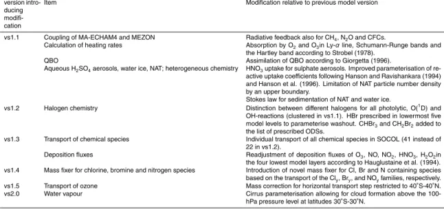
that have been applied to SOCOL vs1.1 concerning halogen chemistry, the transport scheme, and the parameterisation of water vapour. Table 1 gives a summary of the dif-ferences between SOCOL vs1.0 and SOCOL vs2.0. All modifications were performed step by step, represented by the model sub-versions SOCOL vs1.1 to vs1.5. In vs1.2, the halogen chemistry was modified, and in vs1.3–vs1.5, the transport scheme was

20

changed. The difference between vs2.0 and vs1.5 is an improved parameterisation of condensation of water vapour by the highest cirrus clouds.

Although species are transported individually in vs2.0, the nitrogen, chlorine and bromine families are used to modify the mass fixer. In this paper they are defined by molecular number densities as follows:

25

ACPD

Full Screen / Esc

Printer-friendly Version

Interactive Discussion [NO_y] = [NOx] + [HNO3] + [ClONO2] + [BrONO2] + [NAT] (2)

[ClOx] = [Cl] + [ClO] + [HOCl] + 2[Cl2] + 2[Cl2O2] + [BrCl] (3)

[Cly] = [ClOx] + [HCl] + [ClONO2] (4)

[CCly] = [Cly] + [Cl − containing ODS] (5)

[Br_y] = [Br] + [BrO] + [HBr] + [HOBr] + [BrONO2] + [BrCl] (6)

5

[CBry] = [Bry] + [Br − containing ODS], (7)

where [NAT] is the number of HNO3 molecules per air volume condensed inside NAT

particles.

The different model versions are described in the following sub-sections. 4.1 Halogen chemistry (SOCOL vs1.2)

10

In SOCOL vs1.1 the ozone destroying substances (ODS) were grouped into three fam-ilies: short-lived and long-lived organic chlorine containing species, as well as organic bromine containing species. Each of these families was treated as a single species in the chemistry module, using the reaction coefficients of CFC-11, CFC-12, and H1301, respectively. This simplification led to a too slow destruction of the other family

mem-15

bers, their lifetime being shorter than the family representing ones. Consequently, the conversion to inorganic chlorine and bromine was underestimated resulting in too low concentrations of the latter families in the lower stratosphere.

Halogen chemistry in SOCOL vs1.2 is treated more comprehensively by adding 13 photolytic, 14 O(1D)-based, and 8 OH-based oxidation reactions of the type

20

ODS_i + hν → products (8)

ODS_i + O(1D) → products (9)

ACPD

Full Screen / Esc

Printer-friendly Version

Interactive Discussion

ODS_i + OH → products (10)

(ODSi = CFC-11, CFC-12, CFC-113, CFC-114, CFC-115, CCl4, CH3CCl3,

HCFC-22, HC-141b, HC-142b, H1211, H1301, CH3Cl, CH3Br, CHBr3, and CH2Br2) resulting

in an individual chemical treatment of all ODS species in the model. However, to save computational costs the individual treatment of ODS substances is not applied

5

to transport, but the family members are partitioned after each transport step in each grid cell. The fraction P_i of each family member is estimated by the age of air tair,

the (prescribed) concentration of the substance in the planetary boundary layer cbc_i , the number of chlorine and bromine atoms n_i, respectively, and the lifetime of the substanceτci: 10 P_i : = ni[c bc i ]e −tair τci Pn j=1nj[cbc_j ]e −tair τci (11)

The age of air is parameterised to match model results of a tracer study with MA-ECHAM4 (Manzini and Feichter, 1999): The atmosphere is divided into 5 sections, assuming a constant value of age of air in each of these sections. The only time de-pendence is reflected by the online calculation of the local tropopause height according

15

to WMO (1957), which separates the two lowermost sections.

For HBr, a lower boundary condition is introduced in vs1.2 to parameterise tropo-spheric washout: In the lowermost five model layers, HBr is prescribed to amount to 0.1 pptv. In vs1.1, where no lower boundary condition existed, HBr was artificially ac-cumulated in the whole troposphere. Besides, the organic bromine species bromoform

20

(CHBr3) and methylene bromide (CH2Br2) have been added in vs1.2 such that the

model now treats 16 different ODSs.

Figure 1 shows the 1990–1999 zonal mean values of ClO_x, Cl_y, and CCl_yfor the dif-ferent model versions. In general, differences between vs1.1 and vs1.2 are small. The unrealistic features described in Section 1 are visible in both model versions: while total

ACPD

Full Screen / Esc

Printer-friendly Version

Interactive Discussion chlorine (CCl_y) is expected to display an almost constant profile (with small deviations

possibly caused by the time-dependent input of ODS), the simulated stratospheric CCly

in the tropics is up to 30% higher than the maximum tropospheric CCly in vs1.1 and

vs1.2 (Fig. 1b). This feature also appears at high latitudes of both hemispheres during spring and summer, but there it is limited to the upper stratosphere (Fig. 1c, not shown

5

for the Northern Hemisphere). During winter and spring, unrealistic CCly minima

cen-tred at 50 hPa appear at high latitudes, most prominent over Antarctica with values about 50% lower than in the upper stratosphere (Fig. 1a, c, d, e). Another obviously artificial feature is the peak in CCly at the edge of the Southern polar vortex (Fig. 1e).

In contrast to chlorine, bromine species are significantly different between vs1.2 and

10

vs1.1. Due to the newly introduced tropospheric HBr sink, both inorganic bromine (Bry) and total inorganic and organic bromine (CBry) are considerably lower in vs1.2

compared to vs1.1 (30–80% in the middle and lower stratosphere,>95% in the tropo-sphere) (not shown). The artificial accumulation of HBr in the troposphere and lower-most stratosphere present in vs1.1 disappears in vs1.2.

15

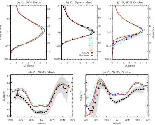
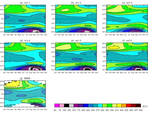
Figures 2 and 3 show zonal means of ozone mixing ratio and column (total ozone), respectively, averaged over the period 1990–1999 for the various model versions in comparison with satellite observations. Slightly higher inorganic chlorine and consid-erably reduced bromine concentrations in vs1.2 compared to vs1.1 result in 15–30% higher ozone abundance in the troposphere (not shown), but have negligible effects in

20

the stratosphere (Fig. 2), except under volcanic conditions, when ozone in the lower tropical stratosphere is reduced by 5–15% (not shown). Total ozone is enhanced by 2– 5% in vs1.2 compared to vs1.1 with a maximum increase over Antarctic in early spring (Fig. 3).

4.2 Transport of all species (SOCOL vs1.3)

25

To save computational costs, the very short lived species were not transported in SO-COL vs1.0–1.2. However, some of the species not transported, such as ClO or Cl₂O₂, led to artificial accumulations in abundance as, for example, it is seen at the edge

ACPD

Full Screen / Esc

Printer-friendly Version

Interactive Discussion of the Southern polar vortex at 70◦S by a peak in CCl_y (Fig. 1e). In SOCOL vs1.3,

the number of transported species has been increased by 19 substances (Cl, ClO, HOCl, Cl2O2, Br, HBr, HOBr, N, NO3, H, OH, HO2, CH3, CH3O, CH3O2, CH2O, HCO,

CH3O2H, O( 1

D)), so that now all 41 species of SOCOL are transported individually. However, the individual transport of all members of the nitrogen, chlorine, or bromine

5

families by a transport scheme that is not mass-conservative requires the application of special measures, such as a family-based mass fixing procedure, to establish mass conservation of the family itself both globally and regionally. Family-based mass fixing has been introduced to SOCOL in vs1.4 and will be discussed in Sect. 4.3.

In vs1.3, both the accumulation of total chlorine (CCl_y) in the middle and upper

strato-10

sphere (Fig. 1b, 1c) and the peak in CClyat the edge of the polar vortex at 70◦S in

win-ter/early spring (Fig. 1e) disappear (green curves). However, transporting all species has no effect on the minimum of CCly at 50 hPa at high latitudes in late winter/early

spring. The reduction of ClOx (and Bry, not shown) concentrations at high latitudes of

the lower stratosphere in vs1.3 compared to vs1.2 result in less efficient chlorine and

15

bromine-induced ozone destruction cycles and to ozone concentrations that are higher than observed (Fig. 2). This effect is most pronounced in the Southern polar vortex (+40–100%; >100% after the eruption of Mt. Pinatubo), see Fig. 2c, e. Compared to vs1.2, ozone is increased by 5–10% (75–100% after Mt. Pinatubo for about two years) in the tropical lower stratosphere and by 5% in the upper stratosphere. Total ozone

20

is increased by 5–10% in the tropics and middle latitudes and by 20% (>50% after Mt. Pinatubo) at the Southern high latitudes in late winter/early spring (Fig. 3).

4.3 Family-based mass fixing (SOCOL vs1.4)

As already stated above, the total chlorine minimum apparent at high latitudes at 50 hPa in late winter/early spring remains even when all species are transported (Fig. 4a).

25

While mass conservation is checked and ensured locally after each chemistry time step, the minimum results from mass loss of CCly (or total bromine, CBry) at high

ACPD

Full Screen / Esc

Printer-friendly Version

Interactive Discussion conservation by the transport scheme, as it will be explained in the following.

The transport of chemical species in SOCOL is calculated using the hybrid numer-ical advection scheme of Zubov et al. (1999), which is a combination of the Prather scheme in flux form (Prather, 1986) for vertical transport and a semi-Lagrangian scheme (Ritchie 1985, Williamson and Rasch, 1989) for horizontal transport. The

5

Prather scheme is strictly mass conservative and ensures to maintain strong gradients (Prather, 1986). However, since the Courant-Friedrichs-Lewy (CFL) stability condition (Courant et al., 1928) has to be satisfied, it is computationally expensive. Therefore, the Prather scheme is only used to calculate the transport in the vertical direction. For the semi-Lagrangian scheme, which is used to calculate the horizontal transport on

10

each model layer, the CFL criterion does not need to be fulfilled. This enables pre-cise treatment of transport near the poles with large time steps (two hours in SOCOL). However, in contrast to the Prather scheme, the semi-Lagrangian scheme is not mass conservative. For this reason a so-called mass fixer has to be used to guarantee con-servation of total mass of each species in each model layer. After each transport step,

15

the transport error ∆ms(k) =

X

i,jms,A(i, j, k) −

X

i,jms,B(i, j, k) (12)

is calculated for every model layer k and every species s, where ms,B(i, j, k) and

m_s,A(i, j, k) are the mass of s in the grid box (i, j, k) before and after the horizontal transport step, respectively. Then, ∆ms(k) is used to scale the mixing ratios of the 20

species µs,A(i, j, k) calculated by the semi-Lagangian scheme. Note that the mass

fixer applied in SOCOL does not correct the individual grid boxes of a layer uniformly, but proportionally to|µs,A(i, j, k) − µs,B(i, j, k)|3/2 (Williamson and Rasch, 1989) to

pe-nalise regions with steep horizontal gradients (which are more critical for errors than regions with almost uniform distributions). Finally, by design, the fixer enables mass

25

conservation only of a whole horizontal layer, but not of individual geographic regions. This may lead to artificial horizontal mass transport and artificial mass loss or accu-mulation in particular regions. Using the mass fixer of Williamson and Rasch (1989) in

ACPD

Full Screen / Esc

Printer-friendly Version

Interactive Discussion SOCOL, regions with steeper horizontal gradients, such as the region of the polar

vor-tex, experience larger corrections and are therefore more vulnerable to artificial mass loss or accumulation.

To better understand the role of the mass fixer for the Southern polar vortex region, we performed idealized tracer simulations with SOCOL vs1.3 using two reciprocally

dis-5

tributed tracers. As initial fields of the simulation, tracer 1 was defined to have a mixing ratio of unity from the South Pole to 83◦S and a mixing ratio of zero between 69◦S and the North Pole. Between 83◦S and 69◦S, the mixing ratio dropped linearly from one to zero. As initial condition for tracer 2, the opposite distribution was used such that the sum of both tracers was unity at all latitudes. The same latitudinal distribution was

10

applied to all altitudes for both tracers. The simulation was started on 1 of September 1996. After one month, the sum of the two tracers, which should ideally remain one everywhere, was found to decrease to about 0.9 in the polar region. We repeated the same simulation with reduced time step and with exponents of 0 or 1 for the mass fixer instead of 3/2 as in Williamson and Rasch (1995). However, the artificial mass loss

15

was found not to improve in these experiments. Next, we used bilinear instead of Her-mite’s spline interpolation to compute the values of the transported gas mixing ratios at the so-called “departure” points of the semi-Lagrangian scheme. This improved the conservation of mass, but led to an undesirable enhancement of numerical diffusion.

Several sensitivity tests were performed to investigate the effects of the mass fixer

20

on chlorine and ozone (all starting 1 January 1996). Table 2 gives an overview over the sensitivity simulations carried out, and Fig. 5 shows their effects on total chlorine (CCl_y), inorganic chlorine (Cl_y), and ozone at 50 hPa and 80◦S. When heterogeneous chemistry is switched off (R2), the artificial mass loss of CCly and Cly is considerably

reduced. Hence, there is strong indication that this effect is caused by the members

25

of the active chlorine family (ClO_x) with steep gradients at the vortex edge. Switching off the mass fixer completely (R3) leads to massive increases in CClyand Cly(Fig. 5a,

b) resulting from artificial mass accumulation. Figure 5c shows that not only chlorine and bromine but also ozone is strongly influenced by the mass fixer. In R1 and R2, at

ACPD

Full Screen / Esc

Printer-friendly Version

Interactive Discussion 50 hPa and 80◦S, the ozone concentration continuously decreases from May to July.

Since there is only little sunlight in the polar region during this period, this cannot have a chemical cause, in particular in R2 with heterogeneous chemistry being switched off. In R3, in contrast, ozone remains more or less constant. From September to December, polar ozone in R3 is considerably lower compared to R2 mainly because of the

artifi-5

cially accumulated Cly. Simulations R4 and R5 show how mass conservation of CCly

and Cl_y can be improved. In these simulations, either CCl_y (R4) or Cl_y (R5) is trans-ported in addition to the individual family members. The mass fixer of Williamson and Rasch is not applied to the individual family members, but to the transported family in-stead. Finally, in every grid box the mixing ratio of the transported and mass-corrected

10

family [f ]∗_T is used to re-scale the mixing ratios of the transported family members [c_i]_T such that the sum of their mixing ratios matches the mixing ratio of the family locally:

[ci]∗_T =

[f ]∗_T PN

j=1nj[cj]T

[cj]T (13)

The suffix∗ depicts mass correction after semi-Lagrangian transportT , ni the number

of chlorine atoms of the family member ci, and N the total number of family mem-15

bers. Basically, this procedure re-introduces a local component to the mass fixer that the standard procedure cannot provide. By applying this method CCl_y (Cl_y) is nearly conserved for R4 (R5), as can be seen from Fig. 5a and b.

In SOCOL vs1.4 we applied the R5 method to obtain mass conservation of the chlo-rine containing species (we did not make use of R4 to avoid conversion of organic

20

chlorine to inorganic chlorine and vice versa). Similarly, family-based mass fixing is used for the bromine and the nitrogen families. For ozone however, since no corre-sponding family exists, this method cannot be applied.

Figure 4 puts this method to test by showing the climatological mean of CCly in

September. Compared to vs1.3 (Fig. 4a), the artificial mass loss in the region of the

25

southern polar vortex is considerably reduced in vs1.4, but still present to a minor de-gree (since family-based mass fixing is only applied to inorganic chlorine, Cl_y, not to

ACPD

Full Screen / Esc

Printer-friendly Version

Interactive Discussion total chlorine, CCl_y). Another deficiency remains with CCl_ybeing slightly higher in the

middle and upper stratosphere than in the troposphere, especially in the tropics. As the fields in Fig. 4b are averaged over 1985–1990, when anthropogenic CFC emis-sions were still increasing, the opposite vertical dependence would be expected. The problem is likely caused by some remaining artificial mass transport of CClyfrom high

5

latitudes to the tropics in the lower stratosphere in late winter/early spring. Via the tropical pipe, this error is transported to the middle and upper stratosphere.

In spite of the remaining shortcomings, the distribution of chlorine is much more realistic in vs1.4 than in vs1.3, which is also evident from Fig. 1. As a result of family-based mass fixing, in vs1.4 CCl_y is increased by 15–25% in the upper and middle

10

stratosphere, as well as in the tropical lower stratosphere (Fig. 1b), and by more than 100% in the region of the polar vortex (Fig. 1a, c–e) in comparison to vs1.3. Like-wise, ClOx is enhanced by 20-120% in the polar vortex, but decreased by 15–20% in

the upper stratosphere (in contrast to CCl_y), especially in the winter hemisphere. This decrease in ClOxis probably caused by an increase of NOy and NOx. Through family-15

based mass fixing, nitrogen oxides are enhanced by 30–70% in the middle and upper stratosphere compared to vs1.3 and reduced by 20% in the lower stratosphere, result-ing in a better agreement with HALOE satellite retrievals (not shown). The low NOyand

NOx abundances in the middle and upper stratosphere in vs1.3 most probably result

from insufficient vertical transport of these substances within the tropical pipe (due to

20

excessive horizontal diffusion of chemical species in the lower stratosphere away from the tropical region towards high latitudes, caused by the Semi-Lagrangian scheme).

Family-based mass fixing also leads to a significant improvement in the distribution of total bromine (CBry) (not shown). In vs1.3, very low mixing ratios of CBrywere found

in the whole stratosphere that amounted to only 20–30% of the tropospheric values

25

leading to an underestimation of observed stratospheric inorganic bromine (Sinnhuber et al., 2005) by about 60%. Similar as for NOy,the low stratospheric CBry abundance

in vs1.3 probably resulted from artificial transport of the bromine containing species from the tropical tropopause to high latitudes by the Semi-Lagrangian scheme, where

ACPD

Full Screen / Esc

Printer-friendly Version

Interactive Discussion they were transported back to the troposphere without having reached the middle and

upper stratosphere. In vs1.4, CBr_yis constant with height to a high degree, except for the region of the polar vortex, where it has a similar minimum as CCly (not shown, for

CClysee Fig. 4b).

The changed spatial distributions of the halogens and the nitrogen oxides strongly

5

affect ozone destruction by the catalytic cycles. As can be seen from Fig. 2d and e, in vs1.4 ozone is decreased by more than 75% compared to vs1.3 in the regions of the polar vortices in both hemispheres and by 10% at middle latitudes of the lower stratosphere, mainly because of increased ClOx (Fig. 1). In the upper stratosphere,

ozone is decreased by 10–15% because of increased NOx. Total ozone is decreased

10

by 5–15% at middle latitudes and by more than 50% in the Southern high latitudes in September and October (Fig. 3c, d). Obviously, vs1.4 total ozone is significantly more underestimated than vs1.3 compared to the New Zealand National Institute of Water and Atmospheric Research (NIWA) observational data set compiled by Bodeker (2005) in the Southern high latitudes in September and October and in the Northern

15

middle and high latitudes in spring. Hence, while family-based mass fixing leads to a significant improvement of modelled chlorine, nitrogen and bromine, the model per-formance with respect to ozone gets worse emphasizing the necessity to additionally investigate the reliability of modelled ozone transport. This will be dealt with in the next section.

20

4.4 Latitudinal restriction of ozone mass fixer to 40◦S–40◦N (SOCOL vs1.5)

For ozone, the family approach described in Sect. 4.3 cannot be applied. Sensitivity tests with the mass fixer switched off for ozone revealed that modelled ozone concen-trations of both hemispheres are highly influenced by the mass fixer. At middle and high latitudes in late winter/early spring, total ozone is significantly increased when the mass

25

fixer is switched off for ozone (not shown) indicating that the too low column ozone val-ues in these regions (Fig. 3c) are at least partly caused by the mass fixer. Qualitatively, the pattern of latitudinal and seasonal variability of zonal mean total ozone fits better

ACPD

Full Screen / Esc

Printer-friendly Version

Interactive Discussion with observations if the mass fixer is switched off for ozone. However, mass

conser-vation is not provided in this case and modelled ozone accumulates artificially in large parts of the stratosphere and troposphere leading to a general overestimation of to-tal ozone when compared to observations. Therefore a possible solution of the mass fixing problem of ozone could be to restrict mass corrections to given geographical

re-5

gions still ensuring global mass conservation on a model layer, but avoiding it in other regions, where the mass fixer produces significant mass loss or accumulation. This methodology was developed based on the results of a sensitivity simulation, by which we show that those regions contributing most to the layer transport error (the global transport error of a certain model layer) are generally not identical with the regions

10

where the mass fixer corrects most. The sensitivity simulation (vs1.4) aimed to quan-tify the contributions of different latitudinal regions to the layer transport error ∆m of ozone caused by the semi-Lagrangian horizontal transport scheme. For this purpose, the globe was divided into nine different latitude belts of 20◦width (70◦S–90◦S, 50◦S– 70◦S etc.). For each latitudinal belt, a corresponding tracer was defined setting its

15

mixing ratio to the ozone value at every grid box within the belt and to a constant value (the zonal mean of ozone at the edges of the belt) elsewhere before each horizontal transport step. As the semi-Lagrangian scheme does not produce an error for constant distributions, the layer transport error ∆mi caused by transport of traceri reflects the

contribution of the_{ith latitude belt to the layer transport error ∆m caused by transport}

20

of ozone.

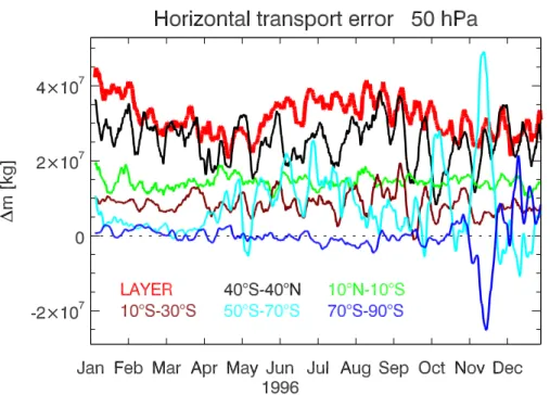
Figure 6 shows the layer transport error ∆m of ozone at 50 hPa, as well as the individ-ual contributions to this error by the tropical belt (10◦S–10◦N), the Southern subtropical belt (10◦S–30◦S), and the Southern high latitudinal belts (50◦S–70◦S; 70◦S–90◦S) as 7-day running mean for 1996. In addition, the transport error produced by the belt

25

40◦S–40◦N is shown. During the whole year, the layer transport error of ozone is pos-itive (red curve), i.e. before corrections by the mass fixer are performed, the global ozone mass in the model layer at 50 hPa is higher after horizontal transport than be-fore. Thus, the mass fixer continuously leads to a downward correction of the mixing

ACPD

Full Screen / Esc

Printer-friendly Version

Interactive Discussion ratios in all grid boxes in this model layer. As can be seen from Fig. 6, the contributions

from the different latitudinal regions to the layer transport error differ in magnitude and depend strongly on season. The contributions of the tropics and subtropics are always positive and do not underlie much annual variability, they probably result from gradients at the edge of the tropical pipe. In contrast, large amplitudes occur in the layer

trans-5

port errors at high Southern latitudes during November and December, most probably related to vortex breakdown. In several months, the transport error of this region is negative indicating that corrections by the mass fixer, based on the full layer, pull sim-ulated ozone systematically into the wrong direction, namely to lower values. This is the main explanation for the significant underestimation of ozone in the region of the

10

Southern polar vortex.

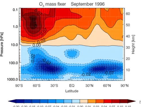
Figure 7 shows the monthly mean of mass fixer corrections for ozone performed after every semi-Lagrangian transport step in September 1996. Below 10 hPa, the mass fixer corrects downward, whereas above 10 hPa, the corrections are upward; the corrections are most pronounced around 200 hPa and 1 hPa. By design of the

15

mass fixer, those regions with the steepest horizontal gradients in every model layer are corrected most. At 200 hPa, these regions coincide with the tropopause, whereas above 100 hPa largest corrections apply to the region of the Southern polar vortex edge. From the sensitivity calculation described above it can be shown that in late winter/early spring the mass corrections are significantly too strong at middle and high

20

latitudes and significantly too weak in the tropics and subtropics at nearly all model layers of the middle and lower stratosphere: This can be understood by the fact that in spite of smaller gradients, the contribution from the tropics and subtropics to the layer transport error is generally larger than from middle and high latitudes, merely because the geographical extent of the tropical region (and thus the mass contained) is much

25

larger than the area of the polar regions. In fact, the error produced by the region 40◦S–40◦N, which contains ∼60% of the area of the sphere, is responsible for the major part of the layer transport error, as shown in Fig. 6.

As consequence, in vs1.5 we restricted the mass fixer of ozone to the region 40◦S– 11121

ACPD

Full Screen / Esc

Printer-friendly Version

Interactive Discussion 40◦N. Hence the middle and high latitudes are not affected by the mass fixer, and the

overall layer transport error ∆m including mass accumulation or loss at middle and high latitudes is fully corrected in the grid boxes between 40◦S and 40◦N, still ensuring global mass conservation on the model layers. (The mass fixing for the other species remains unchanged.) In most seasons and regions, the modelled ozone concentrations

5

are significantly improved with this simple concept as artificial mass loss of ozone at high latitudes is avoided. However, during break-up time of the stratospheric vortices, the transport error is mainly produced at middle or high latitudes (e.g., 50◦S–70◦S in November 1996, Fig. 6). Under these particular circumstances, the transport error would ideally be corrected at high latitudes and not in the tropics showing the limitations

10

of this simple concept.

The restriction of ozone mass fixing to 40◦S–40◦N has a large impact on simulated ozone. In the troposphere and in the lowermost stratosphere, ozone increases by 30– 100% at 40◦S–90◦S and 40◦N–90◦N and decreases by 10–30% at 40◦S–40◦N. As consequence, less Cl is converted to HCl in the polar vortex, as there is more ozone to

15

react with Cl to form ClO leading to an increase of ClO_x by 40–60% compared to v1.4 (Fig. 1c, 1e).

Compared to the NIWA record, simulated total ozone is much improved in vs1.5, es-pecially at high latitudes in late winter/early spring, but also in the tropics and subtropics (Fig. 3). The increase of total ozone at high latitudes in late winter/early spring in vs1.5

20

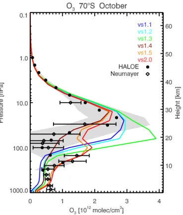
is mainly caused by ozone increases in the model layers below 30 hPa. Figure 8 shows mean ozone molecule number densities at 70◦S in October for the period 1990–1999 for all SOCOL versions, as well as HALOE observations and balloon measurements at the German Neumayer station (Antarctica) over the same period of time. The observa-tions show the well-known profile with a distinct minimum around 50 hPa. In agreement

25

with the observations, vs1.5 has a (less pronounced than observed) minimum at this level, in contrast to vs1.1–1.3 that showed a maximum at around 30 hPa.

ACPD

Full Screen / Esc

Printer-friendly Version

Interactive Discussion 4.5 Improved treatment of water vapour (SOCOL vs2.0)

Water vapour in SOCOL is both treated by the GCM, which includes the complete hydrological cycle in the troposphere, and by the CTM, that accounts for water vapour production/destruction by chemical reactions, but does not parameterise condensation and gravitational settling. At altitudes below 100 hPa, the water vapour field of the CTM

5

is taken over by the GCM (and therefore transported within MA-ECHAM4), whereas above this level, the water vapour field of the CTM is used in the radiation scheme of the GCM and transported like a regular chemical species in the CTM. In contrast to vs1.0– 1.5, vs2.0 takes into account that clouds can also form above 100 hPa in the tropics. In vs2.0, between 30◦S and 30◦N from 40 hPa to 100 hPa, all water vapour exceeding

10

the saturation pressure (calculated after Murphy and Koop, 2005) is removed from the system (by assuming immediate gravitational settling).

As consequence, compared to vs1.0–1.5 simulated water vapour in vs2.0 is reduced by about 30% (≈2 ppbv) above 100 hPa, as shown in Fig. 9. This results in a strato-spheric water vapour abundance that is generally much closer to HALOE observations

15

than in vs1.0–1.5; a relatively small negative bias is a result of a too cold tropical tropopause (∼3 K) in SOCOL. In vs2.0 the lowered stratospheric water vapour con-centrations have a significant impact on stratospheric chemistry: stratospheric HOxis

reduced by 15–25% leading to an increase of methane by 5% (not shown) and to an increase of ozone by 2–5% in the upper stratosphere and lower mesosphere due to a

20

reduction of the catalytic-HOxcycle. The effect on total ozone is small (Fig. 3).

5 Comparison with observations

Simulated and observed ozone is shown in Fig. 2. The shapes of the simulated ozone profiles and latitudinal cross sections are in good agreement with HALOE observations with a maximum (∼10 ppmv) in the tropics at about 10 hPa (Fig. 2b). Compared to

25

vs1.1, simulated ozone in vs2.2 is considerably improved in the middle and high lati-11123

ACPD

Full Screen / Esc

Printer-friendly Version

Interactive Discussion tudes of the lower stratosphere in late winter/early spring (Fig. 2d, e). This can also

be seen from Fig. 8, where ozone molecule number density is shown at 70◦S in Oc-tober. In agreement with the observations, vs1.5 and vs2.0 have a (less pronounced than observed) minimum around 50 hPa, in contrast to vs1.1–1.3 showing a maximum at 30 hPa. Compared to HALOE observations, modelled ozone is overestimated by

5

15–25% in the middle and high latitudes of the summer hemisphere of the lower strato-sphere. In the region of the polar vortex, the bias is positive or negative depending on the month and the model layer. In the tropical lower stratosphere, simulated ozone is around 30% higher than HALOE (Fig. 2d, e), whereas in the upper stratosphere ob-served ozone is generally underestimated by 5–20%. It is noticeable that the layers,

10

where simulated ozone is higher (lower) than HALOE observations, coincide with the layers, where the ozone mass fixer corrects downward (upward), with the transition at about 10 hPa (Fig. 7). It is likely that the biases in simulated ozone are at least partly connected to remaining mass transport artefacts in the semi-Lagrangian scheme.

Total ozone in Fig. 3 is compared with the NIWA record. In agreement with the

ob-15

servations all simulations show the well-known features of highest total ozone values in boreal spring, low total ozone in the tropics with a small seasonal cycle, a relative max-imum in the middle latitudes in late winter/early spring and a minmax-imum ozone column in the Southern high latitudes. While in vs1.1, the winter/springtime maximum at mid-dle latitudes was significantly underestimated in the northern (southern) hemisphere

20

by 5–12% (5–15%), the differences are much reduced in vs2.0 with the northern hemi-spheric maximum now being only 2–5% lower than in the NIWA dataset, and the south-ern hemispheric values even 0–5% higher than in the observations. As consequence of the underestimated springtime ozone maximum, the amplitude of the seasonal cycle in Northern Hemisphere mid-latitude total ozone was underestimated by a factor of two

25

in vs1.1 (not shown). In this respect, the behaviour of the model improved only slightly in vs2.2, still showing a significantly reduced amplitude compared to NIWA (45%). The reduced amplitude of the seasonal cycle in ozone is found in all model layers of the lower stratosphere and is connected to remaining mass fixing problems (Sect. 4.4): a

ACPD

Full Screen / Esc

Printer-friendly Version

Interactive Discussion simulation with the mass fixer completely switched off for ozone showed that the model

is able to simulate a seasonal ozone cycle even more pronounced than observed (not shown). Overall, simulation vs2.0 is closest to observations, and due to restricting the ozone mass fixer to 40◦S–40◦N, it shows a significantly better agreement with NIWA data in the middle and high latitudes of the Northern Hemisphere than vs1.1.

5

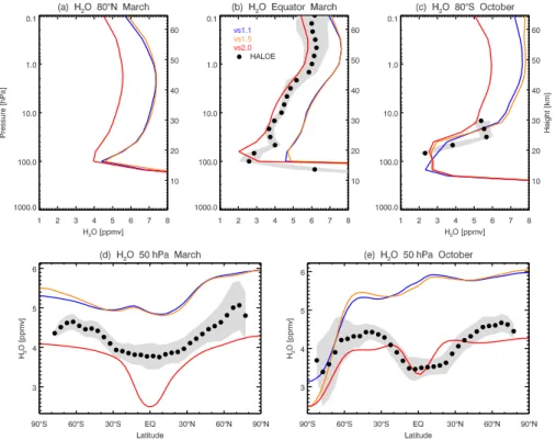
Simulated and observed water vapour is shown in Fig. 9. SOCOL captures the gen-eral shape of the observed stratospheric H2O distribution: mixing ratios increase with

height and with latitude, and are minimal in the polar vortex and near the tropical cold point with lowest values in March (Fig. 9b). Compared to vs1.1, where stratospheric water vapour was generally overestimated by 30–40% compared to HALOE

through-10

out the stratosphere, the overall agreement with observations is much better for vs2.0. With exception of the lower tropical stratosphere, simulated water vapour now has only a slight negative bias (2–12 %) compared to HALOE, mainly as a result of a too cold tropical tropopause (∼3 K) in SOCOL. At 50 hPa, tropical water vapour is underes-timated by more than 30 % compared to observations in vs2.0 during January-May

15

(Fig. 9d), but lies close to observations during August–November (Fig. 9e). This is re-lated to a too fast upward transport of the tape recorder signal in the model combined with a too weak attenuation of the amplitude of the signal (cf. Eyring et al., 2006, their Fig. 9). Consequently, as shown in Fig. 10, the seasonal cycle of simulated tropical water vapour is well captured at the tropical tropopause at 100 hPa, but lies out of

20

phase by 4 months (5.5 months) compared to observations at 50 hPa (30 hPa).

Methane is increased in the whole stratosphere by 5–15% in vs2.0 compared to vs1.1 (not shown) because of reduced HO_x. The decrease of HO_x is caused by the new treatment of water vapour (decreased stratospheric H2O), and by family-based

mass fixing of nitrogen oxides (enhanced formation of HNO3). In the lower and middle

25

stratosphere, simulated CH₄in vs2.0 is only slightly higher (0–10%) than HALOE mea-surements (not shown). However, in the upper stratosphere and in the mesosphere, modelled methane is significantly overestimated in comparison with HALOE (20–50%), which might be related to underestimated methane destruction by the hydroxyl radical

ACPD

Full Screen / Esc

Printer-friendly Version

Interactive Discussion or methane photolysis in the Lyman-α line (not shown).

Furthermore, we compared modelled HCl with HALOE HCl satellite retrievals (Fig. 11). HCl is the most important reservoir species for the chlorine group, and its mixing ratio characterises the total reactive chlorine available for ozone chemistry. The observed increase in HCl with altitude is well captured by SOCOL (Fig. 11b). In the

5

middle and upper stratosphere, HCl is nearly independent of latitude both in obser-vations and in simulations (not shown). In the high Southern latitudes of the lower stratosphere, where HCl was underestimated by 40–80% in vs1.1, the model bias for vs2.0 is significantly reduced (Fig. 11e). In the tropical lower stratosphere, simulated HCl is approximately 40% (50%) higher than observed in March (October) in vs2.0

10

(Fig. 11d, e), which might be connected to remaining mass fixer problems of Cl_y dur-ing the presence of the Southern polar vortex. This overestimation of HCl is partly transported upward into the upper stratosphere, see Fig. 11b.

Finally, Fig. 12 presents total inorganic chlorine (Cl_y) at Southern high latitudes of the lower stratosphere during 1975–2000 for the month of October. Also shown are

15

estimates for Clybased on HCl HALOE measurements (Douglass et al., 1995; Santee

et al., 1996) and the range of Cl_y simulated by all models participating in the CCMVal activity except SOCOL (adapted from Fig. 12b, Eyring et al., 2006). Compared to vs1.1, which participated in the recent CCMVal intercomparison, Clyin vs2.0 is considerably

improved and now lies in the range of the other participating CCMs. Cl_y in vs2.0 is

20

still relatively low, which might be connected to the minimum in total chlorine at high latitudes in late winter/early spring due to remaining mass fixer problems (Fig. 4b).

6 Summary

This paper presented a description of version 2.0 of the CCM SOCOL. In this new model version, most of the shortcomings of version 1.1 described in Eyring et al. (2006)

25

have been eliminated or considerably reduced.

insuffi-ACPD

Full Screen / Esc

Printer-friendly Version

Interactive Discussion cient description of the transport of the chemical species. For instance, unusually high

total inorganic Cl_y concentrations in the middle and upper stratosphere in vs1.1 are caused by an artificial accumulation of ClO not transported in vs1.1. In vs2.0 the num-ber of transported species was increased by 19 to allow all 41 substances of SOCOL to be transported individually. The much too low Cl_y concentrations at high latitudes of

5

the lower stratosphere in winter/early spring in vs1.1 are directly related to the semi-Lagrangian scheme used in the model for horizontal transport. Since this scheme is not mass conserving, a mass fixer according to Williamson and Rasch (1995) is applied after every transport step, which ensures mass conservation of the transported species within each horizontal model layer. However, applying the mass fixer of Williamson and

10

Rasch to each transported species can lead to artificial mass accumulation or mass loss of the respective families (NOy, Cly, and Bry) in particular geographical regions,

most significantly in the region of the polar vortex. In vs2.0, NOy, Cly, and Bryare

trans-ported in addition to the individual family members and their mixing ratios are used to correct the mixing ratios of the members. The method of family-based mass fixing

15

combined with individually transporting all species leads to significant improvement of the nitrogen, chlorine and bromine containing species. Especially in the region of the Southern polar vortex, modelled Clyand HCl are much closer to observations in vs2.0

than in vs1.1.

For ozone, the concept of family-based fixing cannot be applied, as no corresponding

20

family exists. For this reason, to provide an alternative solution, we restrict mass fixing of ozone to 40◦S–40◦N in vs2.0 to take into account that the mass fixer of Williamson and Rasch leads to unjustified corrections of ozone at high latitudes, although about half of the transport error is produced in the tropics and subtropics. Both the modified mass fixer for ozone and the changed catalytic ozone cycles due to modified

distri-25

butions of HO_x, NO_x, ClO_x, and Br_y have a significant influence on simulated ozone. Compared to vs1.1, modelled ozone in vs2.0 is improved especially in the region of the Southern polar vortex, where the simulated vertical ozone profile is much closer to observations.

ACPD

Full Screen / Esc

Printer-friendly Version

Interactive Discussion Stratospheric water vapour, which is overestimated by 30–40% in vs1.1, is

signifi-cantly improved in vs2.0 now taking into account that clouds in the tropics and subtrop-ics can also be formed above 100 hPa. Compared to satellite observations, simulated H₂O of vs2.0 is slightly underestimated mainly because of a cold temperature bias (∼3 K) at the tropical tropopause.

5

The new model version also includes a more comprehensive halogen chemistry treating all chemical reactions of the ODS species individually. However, the influ-ence on chlorine and bromine containing species and on catalytic ozone destruction is relatively low.

Overall, SOCOL vs2.0 shows a significantly improved performance with respect to

10

a more realistic simulation of stratospheric chemical species, most notably for chlorine and water vapour. Hence, the new model version is an appropriate tool for studying a variety of chemistry-climate problems of the middle atmosphere. Due to its good wall-clock performance and the possibility to run the model on regular PCs (one model year requires about two CPU days on state-of-the-art PCs), its main advantage lies in

15

the feasibility to carry out long-term transient ensemble simulations independent from the availability of a supercomputer (e.g., Fischer et al., 20083). We continue to offer the model for use by other research groups without access to large supercomputer facilities.

Acknowledgements. The development and maintenance of SOCOL CCM is part of the project

20

“Variability of the Sun and Global Climate” and funded by ETH Zurich grant PP-1/04-1. VZ was partially supported by the Swiss National Science Foundation (grant SCOPES IB7320-110884). We thank NASA for providing the HALOE satellite retrievals, and the NIWA Data Center for the total ozone data set. The Neumayer ozone sonde data were obtained from the World Ozone and Ultraviolet Radiation Data Centre (WOUDC) operated by Environment Canada, Toronto,

25

Ontario, Canada under the auspices of the World Meteorological Organization.

3

Fischer, A. M., Schraner, M., Kenzelmann, P., Rozanov, E., Br ¨onnimann, S., Peter, T., Griesser, T., Egorova, T., and Schmutz, W.: 20th Century Ensemble Simulations with a Chemistry-Climate Model: Boundary Conditions and Validation, in review for Atmos. Chem. Phys., 2008.

ACPD

Full Screen / Esc

Printer-friendly Version

Interactive Discussion

References

Austin, J., Shindell, D., Beagley, S. R., Br ¨uhl, C., Dameris, M., Manzini, E., Nagashima, T., Newman, P., Pawson, S., Pitari, G., Rozanov, E., Schnadt, C., and Shepherd, T. G.: Uncer-tainities and assessments of chemistry-climate models of the stratosphere, Atmos. Chem. Phys., 3, 1–27, 2003,

5

http://www.atmos-chem-phys.net/3/1/2003/.

Bodeker, G. E., Shiona, H., and Eskes, H.: Indicators of Antarctic ozone depletion, Atmos. Chem. Phys., 5, 2603–2615, 2005,

http://www.atmos-chem-phys.net/5/2603/2005/.

Carslaw, K. S., Luo, B. P., and Peter, T.: An analytic-expression for the composition of aqueous

10

HNO₃-H₂SO₄stratospheric aerosols including gas-phase removal of HNO₃, Geophys. Res. Lett., 22(14), 1877–1880, 1995.

Courant, R., Friedrichs, K., and Levy H.: ¨Uber die partiellen Differenzengleichungen der math-ematischen Physik, Math. Annalen, 100, 32–74, 1928.

Dameris, M., Greve, V., Ponater, M., Deckert, R., Eyring, V., Mager, F., Matthes, S., Schnadt,

15

C., Stenke, A., Steil, B., Br ¨uhl, C., and Giorgetta, M. A.: Long-term changes and variability in a transient simulation with a chemistry-climate model employing realistic forcing, Atmos. Chem. Phys., 5, 2121–2145, 2005,

http://www.atmos-chem-phys.net/5/2121/2005/.

Douglass, A. R., Schoeberl, M. R., Stolarski, R. S., Waters, J. W., Russell II, J. M., and Roche,

20

A. E.: Interhemispheric differences in springtime production of HCl and ClONO2in the polar

vortices, J. Geophys. Res., 100, 13 967–13 978, 1995.

Egorova, T., Rozanov, E., Schlesinger, M. E., Andronova, N. G., Malyshev, S. L., Zubov, V., and Karol, I. L.: Assessment of the effect of the Montreal Protocol on atmospheric ozone, Geophys. Res. Lett., 28, 2389–2392, 2001.

25

Egorova, T., Rozanov, E., Zubov, V., and Karol, I. L.: Model for Investigating Ozone Trends (MEZON), Izvestiya, Atmospheric and Oceanic Physics, 39, 277–292, 2003.

Egorova, T., Rozanov, E., Manzini, E., Haberreiter, M., Schmutz, W., Zubov, V., and Peter, T.: Chemical and Dynamical Response to the 11-year Variability of the Solar Irradiance Simulated with a Chemistry-Climate Model, Geophys. Res. Lett., 83, 6225–6230, 2004.

30

Egorova, T., Rozanov, E., Zubov, V., Manzini, E., Schmutz, W., and Peter, T.: Chemistry-climate model SOCOL: a validation of the present-day climatology, Atmos. Chem. Phys., 5, 1557–