Observations on GEOS-1 of whistler mode turbulence generated by a ground-based VLF transmitter

HAL Id: insu-03206518

https://hal-insu.archives-ouvertes.fr/insu-03206518

Submitted on 23 Apr 2021

HAL is a multi-disciplinary open access

archive for the deposit and dissemination of

sci-entific research documents, whether they are

pub-lished or not. The documents may come from

teaching and research institutions in France or

abroad, or from public or private research centers.

L’archive ouverte pluridisciplinaire HAL, est

destinée au dépôt et à la diffusion de documents

scientifiques de niveau recherche, publiés ou non,

émanant des établissements d’enseignement et de

recherche français ou étrangers, des laboratoires

publics ou privés.

Observations on GEOS-1 of whistler mode turbulence

generated by a ground-based VLF transmitter

T. Neubert, François Lefeuvre, Michel Parrot, N. Cornilleau-Wehrlin

To cite this version:

T. Neubert, François Lefeuvre, Michel Parrot, N. Cornilleau-Wehrlin. Observations on GEOS-1 of

whistler mode turbulence generated by a ground-based VLF transmitter. Geophysical Research

Let-ters, American Geophysical Union, 1983, 10 (8), pp.623-626. �10.1029/GL010i008p00623�.

�insu-03206518�

GEOPHYSICAL RESEARCH LETTERS, VOL. 10, NO. 8, PAGES 623-626, AUGUST 1983

OBSERVATIONS ON GEOS-1 OF WHISTLER MODE TURBULENCE GENERATED BY A GROUND-BASED VLF TRANSMITTER

T. Neubert

Danish Space Research Institute, Lundtoftevej 7• DK-2800 Lyngby• Denmark

F. Lefeuvre• M. Parrot

LPCE/CNRS• 45045 Cedex• Orleans, France

N. Cornilleau-Wehrlin

CRPE/CNET•921311ssy-les-Moulineaux• France

Abstract. Signals launched by the NLK Jim

Creektransmitter in Alaska on 18.60 and 18.65 kHz

have been observed on GEOS-1. Data for one pass over Alaska on June 11, 1977, are presented here. The peak amplitude of the signals is ~5

pT (0.6 mV/m), which is received when the satellite

is close to exact conjugacy at 7500 km altitude. While the weaker signals received at some distance

from conjugacy behave as expected from linear

theory, the stronger signals received closer

to conjugacy have features which indicate that some non-linear process is active. These features

are: 1) a turbulent electric frequency spectrum

2) an increased electrostatic character of the

waves. The threshold field amplitude of the

supposed (but unidentified) non-linear interaction

is ~1 pT.

Introduction

Turbulence of ground based VLF transmitter

signals received by low altitude satellites

at conjugacy in the opposite hemisphere has

been analyzed in Edgar [1976] . Here the

observations are interpreted in terms of linear

propagation effects, where large wave normal

angles produce large Doppler shifts induced

by the satellite motion. In the present case, the satellite and the transmitter are in the

same hemisphere.

The observations are presented in a preliminary

report by Cornilleau- Wehrlin et al. [1978].

They observe a puzzling feature, namely a depression in the cB/E ratio, where c is the velocity of light in vacuum, and B, E the magnetic

and electric field amplitudes of the whistler

waves. This occurs for high field values in

the part of the orbit where the satellite is

close to conjugacy with the transmitter. The depression is rather abrupt, the ratio falling to 1/3 of the values found in the border regions.

It is the purpose of the present paper to extend the analysis and discussion of Cornilleau-

Wehrlin et al. [1978]. First the experimental

set up is described, and the turbulent nature

of the electric signal in the part of the orbit coinciding with the depression in the cB/E ratio is demonstrated. Then calculations of the polarization, ellipticity, and wave normal

direction are presented. Finally the refractive

index and the propagation characteristics are

discussed along with the amplitude calibration of the wave experiment. It is concluded that linear theory is inadequate for describing the

observations. Some suggestions are made for further studies.

The Set Up

The Jim Creek signals are recorded by the

Swept Frequency Analyzer system (SFA) on GEOS-1.

Six SFA's operate as heterodyne systems controlled

by a single frequency synthesizer. The analyzers select bands of 300 Hz in the frequency range

150 Hz to 77 kHz in 256 steps of 300 Hz, thus giving a complete coverage. The sampling frequency

is 1488 Hz, and the bandwidth is determined

by a highpass filter at 150 Hz and a low pass

filter at 450 Hz. When recording the Jim Creek

signals the SFA's were connected to three magnetic

and three electric sensors. The sensors are

parallel to the axis of a cartesian coordinate system with x, y in the spin plane and z along

the spin axis. A more detailed description of

the GEOS wave experiment is found in S-300

Experimenters [1978].

The SFA swept 4 steps around the transmitted

frequencies, recording 0.69 s on each step (1024

samples). This scheme was followed in order to enable the detection of triggered emissions. Such emissions were, however, not observed,

and the present paper uses SFA data from one

step only, covering the frequency range 18.5

to 18.8 kHz.

The Jim Creek transmitter emits coded

information switching between 18.60 and 18.65 kHz.

The minimum duration on either frequency is 10 ms.

Two types of spectral analysis have been

performed. One is a Fourier transform of the 1024 samples from each SFA, producing amplitude

spectra with 1.4 Hz frequency resolution for

each of the 6 wave field components. A spectrum

calculated from a 0.69 s interval will then

contain both frequency components including some sidebands. However, the strongest component in a spectrum will be on either 18.60 or 18.65 kHz if the rays reaching the satellite behave linearly,

and the Doppler shift induced by the satellite motion is negligible.

The other method consists of the construction

Copyright 1985 by the American Geophysical Union. of 3 x 3 spectral matrices of the magnetic field

components, calculated from time averaged modified

Paper number 5L0571.

periodograms [Welch,

1967].

Depending on the

0094-8276/85/005L-0871505.00 time stationarity of the signal, intervals of

624 Neubert et al.' Observation of Whistler Mode Turbulence

0.52 to 0.60 s have been analyzed with a 23 Hz

frequency resolution. This makes it impossible

to discriminate between the two emitted frequencies. Since analysis with a better frequency

resolution gives a poorer signal to noise ratio,

it seems safer to assume that the waves on the two frequencies have the same propagation

characteristics allowing them to mix in the

analysis.

Observations

The rms values of the magnetic and electric

field amplitudes can be calculated from the amplitude spectra. They are shown versus time in Figures la and lb. At 7.30 UT the satellite is approaching the Earth at 10.000 km altitude,

and at 7.55 UT it is located at 5.000 km altitude,

still descending (see Figure 1 of Cornilleau-

Wehrlin et al., 1978). At 7.45 UT the satellite

is at almost exact conjugacy at 7.500 km altitude as calculated from an Olson-Pfitzer model [Kosik, 1978 ].

While the electric signal varies relatively

smoothly, the magnetic signal has large amplitude

variations with conspicuous peaks around 7.36

and 7.42 UT. Figure lc shows the ratio cB/E as function of time. The ratio increases between

7.33 and 7.37 UT as the Jim Creek signal rises

out of the noise. However, the ratio drops abruptly at 7.37 UT from ~4.5 to •2 and decreases further until 7.52 UT where it suddenly rises from ~1

to •3. An exception is the peak at 7.42 UT.

For parallel propagating whistler mode waves the refractive index is given by cB/E. The values shown in Figure lc are, within the depression

region, a factor 4-6 times lower than expected

from theory (see Discussion).

The occurrence of the frequency of the maximum amplitude component in each of the ~700 spectra calculated from 7.25 to 8.00 UT is shown in

5.0 0.0 I I I ..I. . I I - - I , I I J I - cB/E - _ _ I , I , I I o.o 0.6 E E 8.0 c} o.o 7.30 7.40 7.50 8.00 UNIVERSAL TIME (hr)

Figure 1. a) Amplitude of the magnetic field b) amplitude of the electric field c) cB/E.

18.70 ..• 18.65 :• 18.60 18.55 18.70 ,--, 18.65 :• 18.60 18.55 i ' i , i Bx

I

i

I

4

I

I

•

Figure 2. Occurrence of strongest frequency component

Figure 2. From 7.37 to 7.52 UT a few spectral points on Bx appear in between the transmitted

frequencies, signifying a modest state of

turbulence.

The signal on Ey behaves different from that on Bx in the period 7.37 to 7.52 UT, which coincides exactly with the period of depression

in cB/E. The signal is very turbulent, the maximum

spectral component appearing anywhere from 20 Hz below the lower to 30 Hz above the upper of

the two transmitted frequencies.

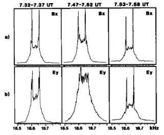
The noisy nature of the signals is illustrated further in Figure 3. Spectra averaged over 5

min are shown for three time intervals: 7.32

- 7.37 UT (not noisy), 7.47 - 7.52 UT (noisy),

and 7.53 - 7.58 UT (not noisy). The spectra

from Bx and Ey are similar in the periods that are not noisy, and resemble spectra calculated from simulated signals. In the noisy period, the Bx spectrum is slightly changed, while the Ey spectrum is very turbulent.

The double peaks on Bx and Ey with a ~5 Hz frequency separation seen on the spectra from

7.32 - 7.37 UT are believed to be an effect caused by two raypaths leading to the satellite in the 5 min period. The wave normal angle of

the rays at the location of the satellite differ and the rays experience different Doppler shifts.

Inspection of individual spectra and Figure

2 indicate that the two ray paths exist

simultaneously.

As a final point in this section the

ellipticity, polarization, and wave normal

direction will be investigated. A detailed analysis

is not possible since measurements of the Earth

magnetic field

Bo, and the plasma frequency

fp do not exist. Still,

some indications can

be obtained from model estimates. Thus B_o is

estimated from a Magsat MGST(6/80) model [Langel

et al., 1980], while fp is taken from Chiu et

al. [ 1979].

The 4 step cycle of the SFA has a 2.75 s period, while the satellite spin has a 5.7 s

period. The satellite

then rotates 43.4 ø during

one step, while the orientation of the xy-antennas

is shifted 173.8 ø each 4 step cycle. For a signal

elliptically polarized in the xy plane, this

results in an amplitude modulation with a period of 80 s.

Neubert eta!.' Observation of Whistler Mode Turbulence 625

The ellipticity of the magnetic wave field in the xy plane at the upper transmitted frequency is found from the rms amplitudes measured on

Bx and By in a 14 Hz band at 18.65 kHz. Using

the fact that the magnetic field of a plane whistler mode wave is circularly polarized in

the plane perpendicular to the wave normal k,

the angle of k to the satellite spin axis can

be found. The result is the curve marked x,

shown in Figure 4a. The points connected with dashed lines suffer from uncertainties due to irregular fluctuations in Bx/By. The same procedure can be used with the signals on Bx and Bz. The result is the curve marked o in Figure 4a. The

analysis is confined to the time interval 7.33

to 7.55 UT where the Jim Creek signal is

predominant.

While the angle to the spin axis may be calculated by the two methods outlined above, the azimuth angle is still unknown. The discrepancy

shown in Figure 4b is then just an indication

of whether the wave field averaged over 40 s

may be considered as plane. This seems to be the case around 7.42 UT and from 7.48 to 7.55 UT.

The results of Figure 4 are to be compared

with the angle of B_o to the spin axis of the

satellite

At 7 30 UT the angle is 75 ø decreasing

to

71 ø at 7.51 UT. Thus, the smallest possible

wave normal angle to B_o

for the periods of plane

waves can be estimated to be ~5 ø at 7.42 UT

and ~15

ø from 7.48 to 7.55 UT.

The polarization of the magnetic field changes

at 7.48 UT which is still in the period of

turbulence. This behaviour is different from

that of the electric field polarization as measured in the xy plane which is well defined during the whole period where the Jim Creek signal

is dominant. The average ellipticity is around 0.5 and unaffected by the degree of turbulence.

The polarization P and ellipticity E have

been estimated from 3 x 3 spectral matrices

of the magnetic field components [Samson and

Olson, 1980] at 66 time intervals in the period

7.32 to 7.53 UT. The wave field can be regarded as that of one plane wave if P > 0.9, while

the ellipticity of plane whistler mode waves

is expected to be close to 1 [Lefeuvre et al.,

1982].

7.32-7.37 UT 7.47-7.52 UT ]'.53-7.58 UT

...

, '" ''"

....

,,,,,,,,,,,,,,,,,,,,,

18.5 18.6 18.7 18.5 18.6 18.7 18.5 18.6 18./' kHz

Figure 3. Averages of spectra (normalized relative to peak amplitude).

Only 7 cases have P > 0.9. These are grouped

around 7.36, 7.42 and 7.48 UT, and coincide

with three of the peaks in the magnetic field

amplitude (Figure la). Note also that they fall

within the regions of well determined polarization

of Figure 4a (solid lines). Furthermore, in

16 cases the analysis shows that the wave field

is left hand polarized, in contradiction to

theory, which predicts right hand polarization.

In Lefeuvre et al. [1982] it was concluded

that the wave normal direction derived from

a spectral analysis is believable only for E > 0.6.

Just one case, at 7.36 UT, meets this requirement.

Here a one peak Wave Distribution Function [Storey

and Lefeuvre, 1979] is found, and the angle

of k to the satellite spin axis determined by

Means

method [Means, 1972] is 73 ø , in reasonable

agreement with the results in Figure 4a.

Two peak WDF's are obtained at 7.32 and 7.41 UT. The solutions are acceptable since the angles of the wave normal to the spin axis derived

from the measured matrices (by Means method)

are almost identical to the ones found from the matrices reconstructed from the WDF solutions.

Also a two peak WDF is consistent with the low

value of P and E found in these cases.

Discussion

The refractive index p of whistler mode waves

may

be expressed on the form: • - f /•f(f

cose-f)

Here f is the wave frequency, fD,fc the electron

plasma and gyro frequencies,-and e the angle

k,B o. With model estimates of fc [Langel et

al., 1980]

and

fp [Chiu

et al., 19791,

refractive

index estimates are calculated and listed in

Table 1 for 8 = 0 ø and 60 ø at three times. In

the table is also listed the maximum expected

Doppler shift &fm = kVs/2•r' where v s is the

satellite velocity.

Outside the depression region, the measured

frequency shift is ~+5 Hz (Figure 3), which

is consistent with the model estimate of the

Doppler shift.

The refractive

index P2 of electromagnetic

waves is given by: •2 = cB/E• where E• is the

component of the electric field perpendicular

to the wave normal k. For parallel propagating

waves (• = 0 ø) E• = E, and a plot like the one

in Figure lc would in this case be a direct

measure of the refractive index. In general

• • 0 ø and as E,,/E• = sin•/(cos•-f/f c), the

refractive index.

The refractive index for parallel propagation

626 Neubert et al.: Observation of Whistler Mode Turbulence

Table 1. Model estimates for three satellite locations. Time (UT) 7.35 7.45 7.55 Altitude (km) 9300 7200 5000 f (kHz) 260 300 370

•c(kHz)

80 120 200

•1 (9=0ø)

7.8

7.0

6.5

•1 (9=6øø)

13.1 10.9 9.6

v s (km/s)

7;7

8.9 10.1

Af.(8=O ø) (Hz)

3.6

3.7

3.9

n•(9=60

ø) (Hz) 6.1 5.8 5.8

than the ratio cB/E of Figure lc in the periods

bordering the depression, and a factor 4-6 larger

within that region. The model parameters are

thought to be reasonable since June 11 was in

a magnetically

quiet period with Kp < 2 during

the previous 24 hours, and GEOS was inside the

plasmapause. Several possibilities are then

open: the amplitude measurements are erroneous,

the waves propagated with very oblique wave normals, and/or the signals behave non - linearly.

The possibility of errors in the calibration of the electric antennas is discussed in Neubert

et al.

[1982], which concludes that the electric

2 to 6, and in Lefeuvre et al. [1982], which

arrive at a factor 3.5.

A factor 2 larger cB/E ratio seems to be consistent with refractive index estimates in

the regions bordering the depression and at

7.42 UT. With the results of the ellipticity

and polarization study it is then concluded

that the signals in these regions behave linearly. Within the depression region the high degree

of turbulence and the electrostatic character

of the waves are consistent with waves propagating with wave normals very close to the resonance

cone, the frequency being Doppler shifted by

the satellite motion (turbulent propagation

vector spectrum). However, it is not possible

to identify the responsible scattering mechanism

since the data set is rather limited. The wave

amplitudes are so large that even local non-linear

wave-wave interactions may be possible [Neubert,

1982•. If this is the case the threshold field

read from Figure 1 is ~1 pT.

We suggest that ISEE-1 and -2 VLF data for

passes near the Aldra Omega station be analyzed.

It should be possible to derive the refractive

index for the 10.2 kHz transmissions.

Acknowledgments. We wish to thank T. Bell

for his helpful suggestions and the information

on the plasma pause position. This work was

supported in part by the Danish Space Board, Danish Natural Science Research Council, and the Otto M•nsted Foundation.

References

Chiu, Y.T.,•J.G. Luhmann, B.K. King, and D.J. Butcher

Jr., An equilibdiummodel of plasmasphere composi-

tion and density, J.Geophys.

Res., 84, 909-916, 1979.

ception of the NLK (Jim Creek) transmitter onboard

GEOS-1,

Space Sci. Rev., 22, 443-451, 1978.

their relation to magnetospheric density structures,

J.Geophys.

Res., 81, 3327-3339, 1976.

Kosik, J.C., The use of past and present magneto- spheric field models for mapping fluxes and calcu-

lating conjugate points, Space Sci. Rev., 22, 481-497, 1978.

Langel, R.A., R.H. Estes, G.D. Mead, E.D. Fabiano, and E.R. Lancaster, Initial geomagnetic field mo-

del from MAGSAT vector data, Geoph¾s. Res.Lett., •,

793-796, 1980

Lefeuvre, F., T. Neubert, and M. Parrot, Wave normal directions and wave distribution functions for

ground-based transmitter signals observed on

GEOS-1,

J.Geophys.Res., 87, 6203-6217, 1982.

riance matrix in analyzing the properties of plane waves, J.Geophys.Res. , 77, 5551-5559, 1972.

Neubert, T., Stimulated scattering of whistler waves by ion acoustic waves in the magnetosphere,

Physica Scripta, 26, 239-247, 1982.

Neubert, T., E. Ungstrup, and A. Bahnsen, Observa- tions on the GEOS-1 satellite of whistler mode

signals transmitted by the Omega navigation system

transmitter in northern Norway, J.Gephys.

Res, 88,

4015-4025, 1983.

Samson, J.C., and J.V. Olson, Some comments on the description of the polarization-states of waves,

Geophys.

J.R.Astron. Soc., 61, 115-129, 1980.

field in a magnetoplasma, 1-the direct problem,

Geophys.

J.R.Astron. Soc., 56, 255-270, 1979.

magnetic wave fields and of cold plasma parameters

on-board GEOS-1, preliminary results, Planet. Space Sci., 27, 317-339, 1979.

Welch, P.D., The use of fast Fourier transform for

the estimation of power spectra: A method based on

time averaging over short, modified periodograms,

IEEE Trans. Audio Electroacoust., 15, 70-73, 1967.

(Received March 14, 1983;