HAL Id: hal-00295258
https://hal.archives-ouvertes.fr/hal-00295258
Submitted on 26 May 2003
HAL is a multi-disciplinary open access
archive for the deposit and dissemination of
sci-entific research documents, whether they are
pub-lished or not. The documents may come from
teaching and research institutions in France or
abroad, or from public or private research centers.
L’archive ouverte pluridisciplinaire HAL, est
destinée au dépôt et à la diffusion de documents
scientifiques de niveau recherche, publiés ou non,
émanant des établissements d’enseignement et de
recherche français ou étrangers, des laboratoires
publics ou privés.
budget for eastern North America
X. Lin, Y. Tao
To cite this version:
X. Lin, Y. Tao. A numerical modelling study on regional mercury budget for eastern North America.
Atmospheric Chemistry and Physics, European Geosciences Union, 2003, 3 (3), pp.535-548.
�hal-00295258�
www.atmos-chem-phys.org/acp/3/535/
Chemistry
and Physics
A numerical modelling study on regional mercury budget for
eastern North America
X. Lin and Y. Tao
Kinectrics, 800 Kipling Avenue, Toronto, M8Z 6C4, Canada
Received: 16 January 2003 – Published in Atmos. Chem. Phys. Discuss.: 20 February 2003 Revised: 17 April 2003 – Accepted: 12 May 2003 – Published: 26 May 2003
Abstract. In this study, we have integrated an up-to-date physio-chemical transformation mechanism of Hg into the framework of US EPA’s CMAQ model system. In addition, the model adapted detailed calculations of the air-surface exchange for Hg to properly describe Hg re-emissions and dry deposition from and to natural surfaces. The mecha-nism covers Hg in three categories, elemental Hg (Hg0), re-active gaseous Hg (RGM) and particulate Hg (HgP). With interfacing to MM5 (meteorology processor) and SMOKE (emission processor), we applied the model to a 4-week pe-riod in June/July 1995 on a domain covering most of east-ern North America. Results indicate that the model simu-lates reasonably well the levels of total gaseous Hg (TGM) and the specific Hg wet deposition measurements made by the Hg deposition network (MDN). Moreover, results from various scenario runs reveal that the Hg system behaves in a closely linear way in terms of contributions from differ-ent source categories, i.e. anthropogenic emissions, natural emissions and background. Analyses of the scenario re-sults suggest that 37% of anthropogenically emitted Hg was deposited back in the model domain with 5155 kg of anthro-pogenic Hg moving out of the domain during the simulation period. Overall, the domain served as a net source, which supplied ∼a half ton of Hg to the global background pool over the period. Our model validation and a sensitivity test further rationalized the rate constant for gaseous oxidation of Hg0by hydroxyl radical OH used in the global scale mod-elling study by Bergan and Rodhe (2001). A further labo-ratory determination of the reaction rate constant, including its temperature dependence, stands as one of the important issues critical to improving our knowledge on the budget and cycling of Hg.
Correspondence to: X. Lin
1 Introduction
Atmospheric Mercury (Hg) exists primarily in inorganic forms with three states, i.e. Hg0(elemental Hg), RGM (re-active gaseous divalent Hg) and HgP (particulate Hg). Al-though the existence of methylated Hg has been reported, it only accounts for less than 3% of the total gaseous Hg, except areas near emissions sources. On the other hand, monovalent Hg (Hg+) is unstable in the atmosphere. Under normal
atmo-spheric conditions, Hg0 is the main component of gaseous Hg, and constitutes the majority of Hg in the atmosphere. RGM is readily dissolved into the water. Subsequently, it is involved in aqueous phase reactions, and is also subject to ad-sorption onto the elemental carbon aerosols. HgP is referred to as particulate solid Hg, which can exist in both gaseous phase and aqueous phase. Now, it is well known that atmo-spheric Hg, predominantly in the gaseous elemental form, has a global atmospheric residence time of about a year. Such a time scale leads to significant long-range transport of the atmospheric Hg and its deposition in the areas distant from major point sources (Fitzgerald et al., 1998). Numeric mod-elling stands as a useful tool to study the complex chemical transformation, transport and deposition processes of atmo-spheric Hg.
Hg is released into the atmosphere from both anthro-pogenic and natural sources. While anthroanthro-pogenic Hg is mainly contributed by chloral-alkali production, coal com-bustion and waste incineration, natural sources of Hg are volcanoes, soils, forests, lakes, rivers and oceans. It was estimated that about 5500 Mg of Hg were emitted globally in 1995 (U.S. EPA, 1997). Recent studies have indicated that Hg re-emitted from various natural surfaces represents a very important part in the atmospheric Hg burden. Mason et al. (1994) suggested a global marine emission of 2000 Mg year−1. Lindberg et al. (1998) estimated an annual emis-sion of 1400 to 3200 Mg of Hg attributable to terrestrial ori-gins (forests and soils). Apparently, in order to gain more
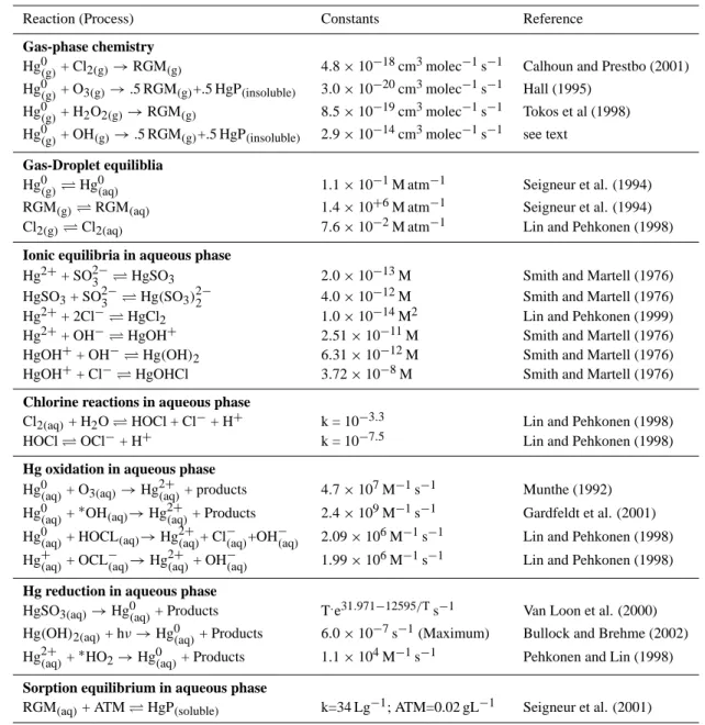
Table 1. The Physio-Chemical Transformation Mechanism of Hg integrated into CMAQ and Associated Rate Constants
Reaction (Process) Constants Reference
Gas-phase chemistry
Hg0(g)+ Cl2(g)→RGM(g) 4.8 × 10⁻¹⁸cm3molec−1s−1 Calhoun and Prestbo (2001)
Hg0(g)+ O3(g)→.5 RGM(g)+.5 HgP(insoluble) 3.0 × 10⁻²⁰cm3molec−1s−1 Hall (1995) Hg0(g)+ H2O2(g)→RGM(g) 8.5 × 10⁻¹⁹cm3molec−1s−1 Tokos et al (1998)
Hg0(g)+ OH(g)→.5 RGM(g)+.5 HgP(insoluble) 2.9 × 10⁻¹⁴cm3molec−1s−1 see text
Gas-Droplet equiliblia
Hg0(g) Hg0(aq) 1.1 × 10⁻¹M atm−1 Seigneur et al. (1994) RGM(g) RGM(aq) 1.4 × 10+6M atm−1 Seigneur et al. (1994) Cl2(g) Cl2(aq) 7.6 × 10⁻²M atm−1 Lin and Pehkonen (1998)
Ionic equilibria in aqueous phase
Hg2++ SO2−3 HgSO3 2.0 × 10⁻¹³M Smith and Martell (1976)
HgSO3+ SO2−3 Hg(SO3)2−2 4.0 × 10
−12M Smith and Martell (1976)
Hg2++ 2Cl− HgCl2 1.0 × 10⁻¹⁴M2 Lin and Pehkonen (1999)
Hg2++ OH− HgOH+ 2.51 × 10⁻¹¹M Smith and Martell (1976) HgOH++ OH− Hg(OH)2 6.31 × 10⁻¹²M Smith and Martell (1976)
HgOH++ Cl− HgOHCl 3.72 × 10⁻⁸M Smith and Martell (1976)
Chlorine reactions in aqueous phase
Cl2(aq)+ H2O HOCl + Cl−+ H+ k = 10−3.3 Lin and Pehkonen (1998)
HOCl OCl−+ H+ k = 10−7.5 Lin and Pehkonen (1998)
Hg oxidation in aqueous phase
Hg0(aq)+ O3(aq)→Hg2+(aq)+ products 4.7 × 10⁷M
−1s−1 Munthe (1992)
Hg0(aq)+∗OH(aq)→Hg(2+aq)+ Products 2.4 × 10⁹M−1s−1 Gardfeldt et al. (2001)
Hg0(aq)+ HOCL(aq)→Hg2+(aq)+ Cl(−aq)+OH−(aq) 2.09 × 10⁶M−1s−1 Lin and Pehkonen (1998) Hg+(aq)+ OCL−(aq)→Hg2+(aq)+ OH−(aq) 1.99 × 10⁶M−1s−1 Lin and Pehkonen (1998)
Hg reduction in aqueous phase
HgSO3(aq)→Hg0(aq)+ Products T.e31.971−12595/Ts−1 Van Loon et al. (2000)
Hg(OH)2(aq)+ hν → Hg0(aq)+ Products 6.0 × 10
−7s−1(Maximum) Bullock and Brehme (2002)
Hg2+(aq)+∗HO2→Hg(0aq)+ Products 1.1 × 10⁴M−1s−1 Pehkonen and Lin (1998)
Sorption equilibrium in aqueous phase
RGM(aq)+ ATM HgP(soluble) k=34 Lg−1; ATM=0.02 gL−1 Seigneur et al. (2001)
accurate insight into the Hg budget and, thereafter, to design suitable abatement strategies, it is imperative to place anthro-pogenic emissions into a proper perspective. In this context, modelling studies on a regional scale need to appropriately include the important component of Hg emissions from nat-ural surfaces.
To study the transport and deposition of the atmospheric Hg in Europe and the United States, several regional mod-elling studies have been carried out. While employing the anthropogenic emission inventories and providing valu-able information on Hg chemistry, transport and deposition, some studies did not include detailed descriptions on the re-emissions of Hg from natural surfaces. In general, the nat-ural re-emissions were either included in the global
back-ground (Bullock et al., 1997; Bullock, 2000; Petersen et al., 1998, 2001; Seigneur et al., 2001) or highly parameterized by a latitude and season dependence (Shannon and Voldner, 1995). Recently, Xu et al. (2000) integrated a Hg component into the Sarmap Air Quality Model (SAQM) (Chang et al., 1996). In their work, a parameterized Hg mechanism similar to the one of Petersen et al. (1995) was adopted. However, significant improvement was made in the estimation of re-emissions of Hg from natural surfaces. Exchanges of Hg be-tween air and the earth surface were explicitly calculated to depict its emissions and dry deposition from and to the sur-faces. Most recently, Bullock and Brehme (2002) developed a regional Hg model based on the framework of a state-of-the science regional air quality model, the US EPA’s Community
Multi-scale Air Quality (CMAQ) model (Byun and Ching, 1999). In their model, a detailed physio-chemical mecha-nism of Hg involving both gaseous and aqueous phases was included to provide a more accurate description of the atmo-spheric Hg in three states (Hg0, RGM and HgP). Again, pre-determined boundary conditions were used to represent the contributions to the atmospheric Hg burden from both global background and natural emissions that originated within the model domain. In the present study, we have further ad-vanced their work by integrating a set of treatments for the atmosphere-surface exchange of Hg. The modelling sys-tem was applied to a domain covering most of eastern North America. This paper describes our model structure, a pre-liminary validation of the model, a quantitative estimation of regional Hg budget and an investigation on the reaction rate constant of the important gaseous oxidation of Hg by hydroxyl radical OH and its impact on the atmospheric Hg modelling practice.
2 Hg mechanism integrated into the CMAQ model sys-tem
CMAQ is an advanced regional air quality modelling sys-tem. It was developed by the Atmospheric Modeling Divi-sion of the U.S. EPA (Byun and Ching, 1999) to simulate the transport, chemical transformation and deposition of air pollutants. Built on a “one-atmosphere” approach, CMAQ is so comprehensive in scope that it allows for the simu-lation of acid deposition, O3 and photochemical oxidants, and fine/coarse particulate matter at spatial scales ranging from urban to regional. CMAQ can be constructed within a computational framework, named Models-3. The frame-work enables users to interact with the modelling system through a high-level graphical user interface. Through the graphics and visualization capabilities, the framework facili-tates data transmission among the components of the system and analysis of model simulation results. However, CMAQ, like its emission preprocessor SMOKE, can also be run in a stand-alone mode by executing scripts, which comprise var-ious UNIX shell commands. In our present study, the stand-alone CMAQ version of June 2001 is utilized as an integra-tion platform. Among the opintegra-tions supported by CMAQ in gaseous phase chemical mechanisms and numerical chem-istry solvers, we selected RADM2 as the chemical mecha-nism and the QSSA solver to solve the stiff chemical system. Further, a physio-chemical transformation mechanism of Hg is integrated into the platform.
The physio-chemical transformation mechanism of Hg in-tegrated into the CMAQ model is presented in Table 1. It is generally similar to the one used by Bullock and Brehme (2002). The mechanism involves Hg in three categories, Hg0, RGM and HgP. Some differences from Bullock and Brehme (2002) in the detailed treatment of the mechanism exist and are worthy to be noted as follows.
1. We assume that particulate mercury consists of two components, a soluble one and an insoluble one. The co-existence of the two HgP components in the atmo-sphere is rationalized by the Hg sorption experiments (Seigneur et al., 1998).
2. Products of gaseous oxidation reactions of Hg0(g) with O3/OH are allocated into two parts, 50% in RGM and 50% in insoluble HgP. The division of the reaction prod-ucts was based on the study by Hall (1995) and the rec-ommendation of Travnikov and Ryaboshapko (2002). 3. A reaction rate constant of 8.7×10⁻¹⁴cm3molec−1s−1
for Hg0(g) oxidation by hydroxyl radical OH was orig-inally reported by Sommar et al. (2001). This rate con-stant together with a normal OH levels would lead to a Hg0lifetime of about 4–7 months. It should be noted that this rate has not been confirmed independently by any other laboratories yet. Travnikov and Ryaboshapko (2002) cautioned the high rate value. Ryaboshapko et al (2002) suggested a further investigation on the rate constant. More significantly, Bergan and Rodhe (2001) used a global model to evaluate the potential role of the oxidation reactions of Hg0. They found that the oxi-dation rate of Sommar et al. (2001) is too large (by about a factor of 3) to reconcile the model calculations with the observed global distribution of Hg0and diva-lent Hg. Based on their findings, we set the rate constant at 2.9 × 10⁻¹⁴cm3molec−1s−1 in the present study. Later on, a sensitivity test on the reaction rate constant will be conducted and discussed in Sect. 5.
4. In addition to its production from the oxidation in gas phase, insoluble HgP is also emitted from anthro-pogenic sources. Dissolved RGM in cloud water is subject to adsorption onto the atmospheric particulate matter. The adsorption leads to the generation of solu-ble HgP that, subsequently, is subject to a desorption process. The resultant sorption equilibrium is repre-sented by an adsorption coefficient (k = 34 L g−1) and an average particulate matter concentration in the cloud droplet of 0.02 g L−1 as recommended by Seigneur et al. (2001).
5. Based on Seigneur et al. (2001), Cl2is set to 10 ppt dur-ing the day; and 100 and 50 ppt for the first layer and the layers above, respectively, at night over the ocean. As for the inland, a zero concentration is assumed. A con-centration of Cl- in the cloud water of 1.0 × 10⁻³g L−1 is adopted from Bullock and Brehme (2002).
It is worth noting that the dry deposition of Hg0was omit-ted in Bullock and Brehme (2002). The modelling study by Xu et al. (2000) suggested that the dry deposition of Hg0 could account for about 20% of the total Hg deposi-tion. In the present study, we calculated the dry deposition
velocity for Hg0using a detailed treatment on the air-surface exchange of Hg0as described in Sect. 4.
3 Anthropogenic emissions of Hg
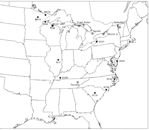
The model domain is shown in Fig. 1. Horizontally, the domain covers most of eastern North America and contains 78 × 67 grids with a grid spacing of 36-km. Vertically, it has 15 layers with varying thickness defined in the ?-coordinates and is stretching from the surface to about 15 000 m above the ground. The anthropogenic emissions of Hg input to the model were compiled using SMOKE (version 1.4B). Two 1995 inventories, the US one and the Canadian one, were utilized in the compilation. The US inventory, acquired from US EPA, cover all three species of Hg for point, area and mobile sources. On the other hand, the Canadian Hg emis-sions inventory, provided by Environment Canada, only in-cludes the emissions for total Hg from point sources. To spe-ciate the total Hg into its three species, we assumed different partitions for different industrial sectors following the treat-ment of Seigneur et al. (2001). More specifically, 56/42/2 of the Hg0/RGM/HgP partition was set for coal-fueled electric utilities; 95/5/0 for chlor-alkali facilities; 85/10/5 for iron-steel industry; 100/0/0 for mining industry; and 50/30/20 for chemical manufacturing industry. The last ratio also served as the default for any sources that were out of the 5 industry categories.
As for the Canadian area and mobile sources of Hg, Envi-ronment Canada has pre-compiled a regional inventory for a 50 km × 50 km grid domain. The Canadian area and mobile emissions were mapped onto the defined model domain. A 50/30/20 partition among the three Hg species was assumed. SMOKE was used to process US area sources, US mobile sources and US/Canada point sources for Hg. These pro-cessed anthropogenic Hg emissions were finally integrated together with the output from normal SMOKE runs for the conventional RADM2 species and the Hg0re-emissions from natural surfaces generated from the process as described in Sect. 4. The integration resulted in netCDF-formatted emis-sion files for inputting to CCTM (CMAQ’s chemical trans-port model, the core model of CMAQ system).
4 Re-emissions and Dry Deposition of Hg0from and to Natural Surfaces
In the present study, we adopted the general approaches of Xu et al. (1999) to calculate the mass transfer (emissions and dry deposition) of Hg0caused by the air-surface exchanges. Briefly, the Penman-Monteith equation for evaportranspira-tion rate (Monteith and Unsworth, 1990) was employed in dealing with Hg0emissions from plant canopies. An empiri-cal relationship between the net Hg0flux at the air-soil inter-face and soil temperature by Carpi and Lindberg (1998), cali-brated by excluding the deposition flux, was used to estimate
the emissions from soils. To calculate the emissions from water, an assumption, that the overall mass transfer coeffi-cient of Hg0 at the air-water interface can be approximated by its mass transfer coefficient in the water, was made. In our view, this assumption can be further rationalized by applying Liss and Slater (1974)’s two-layer model to the interface and is supported by the data provided in Shannon and Voldner (1995) and Poissant et al. (2000).
To facilitate the evaluation of the mass transfer (emissions and dry deposition) of Hg0, we modified MCIP, the meteorol-ogy chemistry interface processor of the CMAQ modelling system, by integrating the algorithms of air-surface Hg0 ex-changes. The modified MCIP generated natural re-emissions and dry deposition velocity of Hg0. One of MCIP’s original output files, METCRO2D, was expanded to include this ad-ditional information. As being input to CCTM runs, the file was also used to generate the netCDF-formatted emission in-put files as described in Sect. 3.
It is worth noting that there are two main differences from Xu et al. (1999) in calculations of Hg0fluxes. The first is related to the quantification of Hg0 content in surface soil water. To compute the emissions from the plant canopies using the evaportranspiration rate, the Hg0concentrations in the surface soil water need to be defined. Xu et al. (1999) set a ”universal” soil water Hg0 concentration such that it had a value of 100 ng l−1for a minimum water stress case. To provide more reasonable geographical variations for the Hg0 concentration, we linked the soil contamination to the deposition of Hg. Because of relatively short lifetimes of RGM and HgP compared to Hgo, we assumed that, as an ap-proximation at the first order, the Hg0content in surface soil water at a concerned location would be proportional to the product between the strength of a contributing anthropogenic RGM/HgP source and the squared reciprocal of the distance between the contributing source and the concerned location. A geographical distribution of the summed product was then generated by adding the contributions from all anthro-pogenic RGM and HgP sources within the modelling domain for each grid of the domain. According to the field study of Poissant and Casimir (1998), the Hg contents in surface soil water in southern Quebec, as derived from measured fluxes of Hg and water vapour, were about 15 ng L−1. This value was used to calibrate the summed variables to create a ge-ographical distribution of Hg0content in surface soil water for the modelling domain. The resultant distribution gives 70 ng L−1 of Hg0 in soil water for east-central Tennessee. This level is adequate to explain the observed emission rates from plant canopies (Lindberg et al., 1998). There is an un-certainty associated with the determination of the Hg0 con-tent. As to be seen later, the re-emissions of Hg0only ac-count for a small part (∼2%) of wet deposition over the entire domain due to the physio-chemical nature of Hg0. Therefore, we do not expect that the uncertainty involved would lead to a substantial difference in the wet deposition simulation of Hg.
Figure 1. The model domain. Also shown are the site locations of measurements used to evaluate the model performance (see text for details).
Fig. 1. The model domain. Also shown are the site locations of measurements used to evaluate the model performance (see text for details).
The second difference lies in the estimation of the mass transfer coefficient of Hg0, Kw, in water when calculating the air-water exchanges. While Xu et al. (1999) used em-pirical formulae of Mackay and Yeun (1983) and Asher and Wanninkhof (1995), we adopted the approach by Poissant et al. (2000). Briefly, Kw(cm h−1) can be correlated with the mass transfer of CO2 across the airwater interface through (Wanninkhof et al. 1985, Hornbuckle et al., 1994)
Kw= (0.45 U101.64)[Scw(Hg0) / Scw(CO2)]0.5
where U10 is the wind speed (m s−1) at 10 m and Sc’s are the Schmidt numbers for CO2 and Hg0 in water, respec-tively. The Schmidt number of CO2is calculated using the temperature-corrected dependency (Hornbuckle et al., 1994; Bidleman and McConnell, 1995)
Scw(CO2)= 0.11 T2−6.16 T + 644.7
with T in◦C. The Schmidt number of Hg0is directly derived from its definition
Sc = ν/D
where the temperature (◦C) dependant ν (kinematic viscos-ity of water, cm2s−1) and D (diffusivity of Hg0 in water, cm2s−1) are estimated by
ν =0.017 exp(−0.025 T ) (Thibodeaux,1996)
D =6.0 × 10⁻⁷T +10−5 (Kim and Fitzgerald, 1986)
The re-emissions of Hg0 in the model domain accumu-lated over a 4-week period from 20 June 1995 to 18 July
1995 are presented in Fig. 2. It is seen that the re-emissions substantially diminish in the northern part of the model do-main. This is partially due to minimized agricultural cov-erage in the regions. As Xu et al. (1999) indicates, re-emissions from agriculture are significantly larger than the re-emissions from forest and other land-use categories. The land-use effect is further enhanced by a less mercury con-tent in surface soil water owing to much less anthropogenic sources than in the southern regions. In the eastern part of the model domain, relatively high re-emissions over the At-lantic Ocean coincide with higher average wind speed (not shown here). It is the high wind speed that causes the rela-tively high re-emissions through the wind dependence of the air-water exchange stated above.
5 Model runs, results and discussion
In the study, we carried out the regional Hg modelling for the time period of 16 June 1995 to 18 July 1995. The modelling procedure started with a normal run of the meteorological processor MM5, a modified MCIP run and a normal run of the emission processor SMOKE. Then, a second SMOKE run with Hg emission inventories was conducted before exe-cuting the modified CCTM for Hg. To account for the global background of Hg, we set boundary conditions of 0.2 ppt for
Figure 2. Total re-emissions of Hg0 (ng m-2) from natural surfaces over the period of 20 June 1995 to 18 July 1995.
Fig. 2. Total re-emissions of Hg0(ng m−2) from natural surfaces over the period of 20 June 1995 to 18 July 1995.
Hg0, 0.01 ng m−3for both RGM and HgP. These background levels are similar to the ones chosen by Bullock and Brehme (2002) and Xu et al. (2000). The same values were assigned for Hg initial conditions. Although our model runs covered a 32-day period, the results from the first 4 days were ex-cluded from analysis to avoid the unstable data in the initial “warm-up” period of a normal numerical modelling practice. To facilitate analysis, we conducted runs for 4 different sce-narios. The 4 scenarios are
1. S0, a base-line scenario, which includes both anthro-pogenic emissions and re-emissions of Hg from natural surfaces as well as Hg boundary conditions;
2. Sba, the same as S0but without re-emissions of Hg from natural surfaces;
3. Sbn, the same as S0 but without anthropogenic emis-sions of Hg; and
4. Sb, the same as S0but without both anthropogenic emis-sions and re-emisemis-sions of Hg from natural surfaces. 5.1 Model validation
To have a preliminary evaluation of the regional Hg model, we compared the model results from the S0run with the mea-sured ground level concentrations of total gaseous Hg (TGM) (Fitzgerald et al., 1991; Burke et al., 1995; Lindberg and
Stratton, 1998; Blanchard et al., 2002) and Hg wet depo-sition at the sites of Hg depodepo-sition network (MDN) (Lind-berg and Vermette, 1995; http://nadp.sws.uiuc.edu/nadpdata/ mdnsites.asp). The measurement sites are plotted in Fig. 1 together with the model domain. While the TGM measure-ments represented general long-term averaged values, the MDN’s data used in the study were those taken from June– July of 1995. Since our model runs covered a period from 20 June 1995 to 18 July 1995 after excluding the “warm-up” period of model initiation, we can make a direct comparison between the modelled wet deposition of Hg and the MDN data.
For an illustration purpose, we plotted the total wet de-position of Hg over the 4-week period calculated from the S0 run in Fig. 3. In parallel, the total precipitation over the same period, which was derived from MM5 runs and was in-put into CMAQ, is plotted in Fig. 4. While the two variable fields show similar distribution patterns, some differences in the intensity exist in the east coastal and some central US re-gions. This disparity can be explained by the distribution of anthropogenic emission sources. It is known that the major-ity of Hg wet deposition are attributable to RGM and HgP and that the concentrations of RGM and HgP peak in the vicinities of the sources due to their relatively short lifetime. Therefore strengthened anthropogenic emissions in these re-gions, as shown in Fig. 5, compensated the relatively small precipitation and eventually led to significant wet deposition.
Table 2. Comparisons of Modelled Total Wet Deposition of Hg and Averaged Ground Level Concentration of TGM over the Four-Week
Modelling Period with Measurements
Wet Deposition of Hg over Ground Level Concentration of TGM Averaged 20 June 1995–18 July 1995 over 20 June 1995–18 July 1995
MDN Obs. Site Obs. Value (ng m−2) Model Value (ng m−2) Obs. Site Obs. Value (ng m−3) Modelled Value (ng m−3)
DE02 1044 1335.2 Egbert, ON 1.8 1.80
(Blanchard et al., 2002)
KY99 994 981.9 Burnt Island, ON 1.7 1.76
(Blanchard et al., 2002) NC08 1538 2225.7 Point Petre, ON 2.0 1.80 (Blanchard et al., 2002) NY97 2120 2097.2 Underhill, VT 1.9 1.71 (Burke et al., 1995) SC19 2129 2433.1 Trout Lake, WI 1.6 1.66 (Fitzgerald et al., 1991)
WI36 1754 1292.0 Walker Branch Watershed, TN 2.2 1.88 (Lindberg and Stratton, 1998)
Figure 3. Calculated total wet deposition of Hg0 (ng m-2) over the period of 20 June 1995 to 18 July 1995.
Fig. 3. Calculated total wet deposition of Hg0(ng m−2) over the period of 20 June 1995 to 18 July 1995.
Table 2 presents the comparisons of our model results from the scenario S0run with the field measurements. For ground level concentrations of TGM, the model results including both Hg0 and RGM were averaged over the modelling pe-riod. It is seen that the averaged TGMs derived from the model agree well with the measurements. In general, the modelled results are within 10% of the observations. As for the wet deposition of Hg, six MDN sites reported valid total
wet deposition of Hg for the entire 4-week modelling pe-riod. As shown in Table 2, the model did reasonably well in simulating the measured total wet deposition. The rela-tive simulation errors lie between −26% and +45%. Since MDN sites were usually measuring the Hg wet deposition on a weekly basis, analysis was also conducted for the weekly data. Among all MDN sites, there are 35 valid weekly de-position data involving 11 sites during the 4-week period.
Figure 4. Total precipitation (cm) over the period of 20 June 1995 to 18 July 1995, as inputted to CCTM.
Fig. 4. Total precipitation (cm) over the period of 20 June 1995 to 18 July 1995, as inputted to CCTM.
Figure 5. Total anthropogenic emissions of RGM and HgP (ng m-2) over the period of 20 June 1995 to 18 July 1995, as inputted to CCTM.
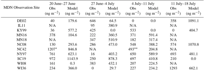
Table 3. Comparisons of Modelled Weekly Wet Deposition of Hg with Measurements from 11 MDN Sites
20 June–27 June 27 June–4 July 4 July–11 July 11 July–18 July MDN Observation Site Obs Model Obs Model Obs Model Obs Model
(ng m−2) (ng m−2) (ng m−2) (ng m−2) (ng m−2) (ng m−2) (ng m−2) (ng m−2)
DE02 40 179.6 646 64.5 0 0.0 358 1091.1
IL11 N/A 95 380.9 N/A N/A
KY99 36 577.2 425 0.0 533 0.0 0 404.7 MN16 378 104.6 222 360.5 371 591.4 N/A MN18 N/A 347 510.9 182 317.4 N/A NC08 130 293.6 286 473.0 548 388.2 574 1070.8 NC42 1207∗ 846.8 N/A 493∗∗ 204.8 N/A NY97 761 623.1 16 403.2 650 589.9 693 481.1 SC19 972 1143.9 250 878.3 697 410.8 210 0.0 WI08 161 0.3 383 432.1 207 224.5 N/A WI36 234 366.0 0 29.7 227 234.2 1293 662.1
∗Sample dates 22 June 1995 to 29 June 1995 ∗∗Sample dates 06 July 1995 to 13 July 1995
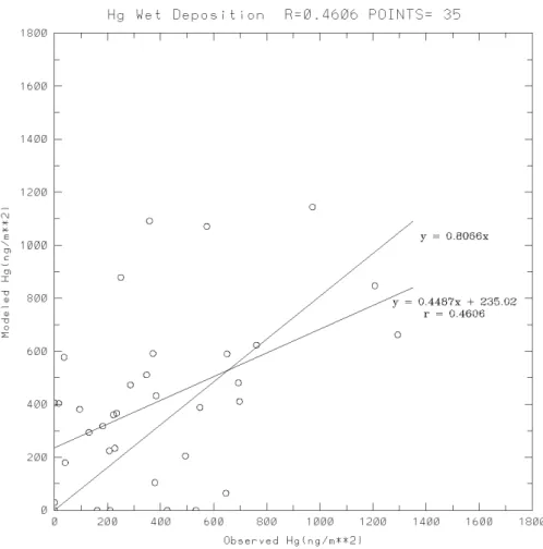
The weekly data of the 11 sites are listed in Table 3 together with their modelled counterparts. A scatter plot with a least-squares regression line and a forced regression line with zero intercept is presented in Fig. 6. This plot is indeed paral-lel to Fig. 5b of Bullock and Brehme (2002). The present calculated correlation coefficient is 0.46, indicating an im-provement over the correlation coefficient 0.329 by Bullock and Brehme (2002). More comparisons of statistics are sum-marized in Table 4. While Bullock and Brehme (2002) sig-nificantly over-predicted the mean value and the variability of the measured data, the present study improved the two statistics with a slight over-estimation of 5.2% and a slight under-estimation of 2.6%, respectively. The improvement is reflected in all 4 quartiles.
The overall improvement mainly resulted from the re-duced rate constant of the gaseous oxidation of Hg0by OH. As to be shown in a sensitivity analysis below, a reduction of the rate constant by two third of the value originally reported by Sommar et al. (2001) leads to a considerable decrease of ∼5000 kg in the total wet deposition over the simulation do-main for the entire modelling period. At the same time, as a regional budget analysis in the next section indicates, this decrease is compensated by a small increase (180 kg) in the wet deposition due to the inclusion of the re-emissions from natural surfaces.
Despite the overall improvement introduced by a 3-fold reduction of the critical rate constant, the correlation coef-ficient between the measured and the modelled wet depo-sition of Hg is still low. As pointed out by Bullock and Brehme (2002), the wet deposition simulation is directly af-fected by the input meteorological data. For the above 35 weekly cases, we analyzed the correlation between the real precipitation depth (cm) and the input precipitation depth. While the real data were retrieved from wet deposition data
(ng m−2) and samples’ concentration data (ng L−1) for Hg, the model input was generated from MM5 runs. An analy-sis on the pair of precipitation data led to a Pearson corre-lation coefficient of 0.36, which is comparably low with the one for the wet deposition of Hg. On the other hand, the linear correlation analyses on the wet deposition of Hg and the precipitation depth resulted in Pearson correlation coef-ficients of 0.83 for the MDN measurement data and 0.72 for the model input/output. Evidently, an improvement in the modelled precipitation field would significantly improve the model performance for the wet deposition simulation of Hg. 5.2 Regional budget
To investigate the regional budget of Hg, we calculated the domain total deposition of Hg over the modelling period of 20 June 1995 to 18 July 1995. The calculations were done for each of the 4 scenarios defined above. The resultant total deposition for all three components of Hg is presented in Ta-ble 5. The deposition was further segregated into the dry part and the wet part. Also shown in the table are total emissions released from the sources within the model domain during the simulation period. From the table, re-emissions of Hg from natural surfaces account for 60% of total Hg emissions or 1.5 times of anthropogenic Hg emissions. It is of interest to note that the Hg system behaves in a nearly linear way. Based on the four scenario definitions, the close linearity can be illustrated by comparing the summed value of S0and Sb with the summed value of Sba and Sbn for each of the de-position categories in Table 5. By subtracting the value of a variable in Sbfrom its counterpart in another scenario, we estimated contribution to the variable from an emission com-ponent, which was added onto the Sbto form the other sce-nario. More specifically, we calculated the contributions to
Figure 6. Scatter plot of modelled versus measured wet deposition of Hg. Also shown are a least-squares regression line and a forced regression line with zero intercept.
Fig. 6. Scatter plot of modelled versus measured wet deposition of Hg. Also shown are a least-squares regression line and a forced regression
line with zero intercept.
Table 4. Comparison of Statistics among MDN Measurements, Results of Bullock and Brehme (2002), Results from Baseline Run and
Results from Sensitivity Test Run (see text for detail)
Sample # Data Source Mean (ng m−2) σ Min. (ng m−2) Percentile (ng m−2) Max. (ng m−2) 25th 50th 75th
35 MDN Measurement 389.3 327.3 0.0 171.5 347.0 561.0 1293.0 35 Bullock and Brehme (2002) 623.7 621.1 0.0 202.1 482.5 759.7 2598.5 35 Baseline Run 409.7 318.9 0.0 192.2 388.2 583.5 1143.9
dry/wet deposition from anthropogenic emissions plus nat-ural re-emissions, anthropogenic emissions only and natu-ral re-emissions only, respectively. The estimated values are listed in the brackets in Table 5. In addition, the re-emissions and deposition of Hg from and to natural surfaces associ-ated with the base-line scenario run are presented in Table 6. From the two tables, one may observe the followings.
1. Among 8216 kg of Hg emitted anthropogenically, 3061 kg (37.3%) were directly deposited back in the domain. Accordingly, 62.7% of anthropogenic Hg (5155 kg) moved out of the domain and, subsequently
were integrated into the background. This partition is similar to U.S. EPA (1997).
2. Among 12 481 kg of naturally re-emitted Hg, 704 kg (5.6%) were directly deposited back in the domain with 180 Kg deposited though the wet process. A majority part (94.4%) of the re-emitted Hg moved out of the do-main and was integrated into the background.
3. The background contributed 16 477 kg of Hg deposition in the domain, accounting for 81.4% of total deposition.
Table 5. Domain Total Deposition of Hg Calculated over the Period of 20 June 1995 to 18 July 1995 from Four Scenario Runs
19
Table 5. Domain Total Deposition of Hg Calculated over the Period of 20 June 1995 to 18 July 1995 from Four Scenario Runs
Dry Deposition over Entire Domain (Kg)
(Bracketed values refer to differences from the Background Scenario Sb)
Wet Deposition over Entire Domain (Kg)
(Bracketed values refer to differences from the Background Scenario Sb)
Scenarios Emis.within Domain (Kg) Hg0 RGM HgP Hg0 RGM HgP 6068 4277 159 1 3683 6048 10503 (2230) 9733 (1529) S0: Base Line 20697 20236 (3759) 5637 4192 155 1 3612 5940 9985 (1712) 9554 (1350) Sba: Background+ Anth. Emis. 8216 19538 (3061) 5921 2751 125 1 3154.6 5228 8797 (524) 8384 (180) Sbn: Background+ Re-Emis. 12481 17181 (704) 5485 2666 121.5 1 3082.5 5120 8273 8204 Sb: Background only 16477
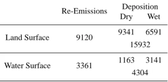
Table 6. Re-emissions and Deposition of Hg over the Period of 20 June 1995 to 18 July 1995 in the Base-Line Scenario Simulation.
Deposition Re-Emissions Dry Wet 9341 6591 Land Surface 9120 15932 1163 3141 Water Surface 3361 4304
Table 7. Statistics Comparison between Baseline Run and Sensitivity Test Run Bias
(ng m-2)
Error
(ng m-2) RelativeBias RelativeError
RMSE (ng m-2) Index of Agreement Baseline (S0) Run 20.4 267.2 1.51 2.02 331.5 0.6745 Sensitivity Test Run 262.5 399.6 2.97 3.33 518.0 0.5996
4. While background contributions predominated, anthro-pogenic emissions contributed more than 5 and 7 times than the re-emissions to the dry deposition and the wet deposition, respectively.
5. While a total of 20 697 kg of Hg was emitted, 20 236 kg of Hg were received by the surface within the domain through deposition processes. This resulted in a net loss of about a half ton and, therefore, indicates the domain as a whole acting as a net supplier to the background pool of Hg for the 4-week simulation period. However, this “net source” conclusion should be dealt cautiously. The net contribution to the background pool only ac-counts for about 2% of the amount of Hg received or the amount of Hg emitted in the domain, and repre-sents indeed a small difference between the two large numbers. Considering the uncertainties inherited in the study (such as the anthropogenic emission inventory, the formulation of re-emissions and dry deposition pro-cesses, and the precipitation field etc.) the sign of the small difference could be changed as some input data were altered.
6. As the cycling of Hg is concerned, the data in Table 6 indicate that the land surface within the model domain re-emitted 9120 kg of Hg while received 15 932 kg of Hg during the 4-week simulation period. For the water surface, the re-emissions and deposition were 3361 kg and 4304 kg, respectively. The Hg surplus status at the natural surfaces indicates an ongoing accumulation pro-cess in the land and the water, and is consistent with the general picture of the human and industrial activities in the region.
Table 6. Re-emissions and Deposition of Hg over the Period of 20
June 1995 to 18 July 1995 in the Base-Line Scenario Simulation Deposition Re-Emissions Dry Wet Land Surface 9120 9341 6591 15932 Water Surface 3361 1163 3141 4304
5.3 Sensitivity of rate constant of gaseous oxidation by OH As mentioned previously, in their global modelling study, Bergan and Rodhe (2001) found that the rate constant of gaseous oxidation by OH of Sommar et al. (2001) is too large by about a factor of 3 to simulate the observed global distribution of Hg0 and divalent Hg. Based on their find-ings, we set the rate constant at 2.9 × 10⁻¹⁴cm3molec−1s−1 in the study. To shed light upon the impact of the rate constant on the model simulations, we reset the rate at 8.7 × 10⁻¹⁴cm3molec−1s−1and run the CCTM with emis-sions, initial/boundary conditions and all other inputs kept at the same values as Scenario S0. Results indicated that the fast oxidation reactions led to more production of RGM and HgP. Consequently, more dry and wet deposition was generated at the expense of Hg0. Over the entire modelling period, the domain total dry and wet depositions were 12 068 kg and 14 960 kg, respectively. These numbers represent a 15.9% in-crease of the dry deposition and a 53.7% inin-crease of the wet
Table 7. Statistics Comparison between Baseline Run and Sensitivity Test Run
Bias (ng m−2) Error (ng m−2) Relative Bias Relative Error RMSE (ng m−2) Index of Agreement Baseline (S0) Run 20.4 267.2 1.51 2.02 331.5 0.6745
Sensitivity Test Run 262.5 399.6 2.97 3.33 518.0 0.5996
deposition. Accordingly, the domain averaged ground level concentration of TGM dropped by 0.054 ng/m3(3.2%) from the S00s value. Under this circumstance, the domain would serve as a strong sink in the sense of a global budget with a net gain of 6331 kg of Hg. This net gain would be equiva-lent to 30.6% of the amount emitted both anthropogenically and from natural surfaces within the domain. Evidently, such a large positive percentage is not consistent with the human and industrial activities within the region in a global context. The model results from the sensitivity test run were also compared against the measurements. The calculated ground level concentrations of TGM for the 6 observation sites were 0.04–0.08 ng/m3less than their counterparts from the S0run. The drops in such a range did not practically weaken the model performance for TGM. The simulation of the wet deposition measurement, however, was significantly deteri-orated. To illustrate the deterioration, we calculated bias, error, relative bias, relative error, root mean squared error (RMSE) and index of agreement (IOA) for model results from both the S0run and the sensitivity test run. While bias, error, relative bias, relative error and RMSE follow their con-ventional definitions; IOA is defined as
I OA =1 − N (RMSE) 2 M P i=1 (|Mi0| + |Oi0|)2
where N is the total number of samples, Mi0 and Oi0 are
the departures from the mean observed value of the mod-elled value and the observed value, respectively. A value of IOA=1 indicates a perfect agreement and IOA=0 indicates absolutely no agreement (Hedley et al., 1995). Calculated statistics are shown in Table 7. It is seen that the tripled rate constant caused much higher wet deposition of Hg at the MDN sites and worse agreement with the measurements than the S0run. As shown by the values of bias, the mean value of the 35 samples would be 262.5 ng/m2 higher than the measured mean compared to 20.4 ng/m2higher in the S0 case. This over-prediction is even larger than the overesti-mation of 234.4 ng/m2 by Bullock and Brehme (2002) (as seen in Table 4), apparently due to the inclusion of the Hg re-emissions from natural surfaces in the study.
6 Conclusions
In the present study, we integrated an up-to-date physio-chemical transformation mechanism of Hg and detailed
cal-culations on the air-surface exchange of Hg0into the frame-work of US EPA’s CMAQ model system. An application of the constructed Hg model to a 4-week period in June/July 1995 indicated that the comprehensive model simulated rea-sonably well the specific wet deposition measurements of Hg at the MDN sites as well as the general ground level concen-trations of TGM. Results from various scenario runs revealed that the Hg system behaves in a closely linear way in terms of the source contributors, i.e. anthropogenic emissions, nat-ural emissions and background. Analyses on model re-sults showed that 37% of anthropogenically emitted Hg were deposited back in the model domain with 63% (5155 kg) of anthropogenic Hg moving out of the domain during the sim-ulation period.
The results from the base-line run indicated that the do-main as a whole served as a net source to supply about a half ton of Hg into the global background pool over the sim-ulation period. This amount represents about 2% of the Hg amount received by the surfaces or the amount of Hg emitted in the domain. Considering the uncertainties involved, the sign of the small net source could be changed, as some in-put data would be altered. Moreover, the global background contributed more than 80% of the regional deposition of Hg. The background dominance reflects the “long-living” nature of Hg. Consequently, it implies that a proper Hg modelling needs to be performed on a large spatial scale such as a con-tinental scale unless boundary conditions can be defined rea-sonably well.
It should be noted that the present study is subject to lim-itations or uncertainties as any similar modelling studies. These limitations or uncertainties are ranged widely from emissions, meteorology prediction, mechanism description, and deposition treatment to lack of dry deposition compari-son. Following other significant pioneer works, we carried out this comprehensive regional modelling study by includ-ing the up-to-date physio-chemical transformation mecha-nism of Hg and the up-to-date treatment of Hg re-emission and dry deposition. Through the model validation and a sen-sitivity test, it emerges that the currently reported reaction rate constant of the gaseous oxidation of Hg0 by hydroxyl radical OH could be too large by a factor of 3. Therefore, a further laboratory determination of the rate constant, in-cluding its temperature dependence, stands as one of the important issues critical to improving our understanding on the budget and cycling of Hg. On the other hand, the present model will also benefit from more field studies on
the air-surface exchange of Hg0. These studies will provide much valuable information to modify/ correct the assump-tions or parameters employed in the model study such as the Hg content in surface soil water etc.
References
Asher, W. E. and Wanninkhof, R.: The effect of breaking waves on the analysis of dual-tracer gas exchange measurements, in Air-Water Gas Transfer, (Eds) Jhne B. and Monahan E. C., Aeon Verlag, Hanau, pp. 517–528, 1995.
Bergan, T., Gallardo, L., and Rodhe, H.: Mercury in the global troposphere: a three-dimensional model study, Atmospheric En-vironment, 33, 1575–1585, 1999.
Bergan, T. and Rodhe, H.: Oxidation of elemental mercury in the at-mosphere; Constraints imposed by global scale modelling, Jour-nal of Atmospheric Chemistry, 40, 191–212, 2001
Bidleman, T. F. and McConnell, L. L.: Gas exchange of persistent organic pollutants, Science of the Total Environment, 159, 101– 117, 1995.
Blanchard, P., Froude, F. A., Martin, J. B., Dryfhout-Clark, H., and Woods, J. H.: Four years of continuous total gaseous mercury (TGM) measurements at sites in Ontario, Canada, Atmospheric Environment, 36, 3735–3743, 2002.
Bullock, O. R. Jr., Benjey, W. G., and Keating, M. H.: The modeling of regional-scale atmospheric mercury transport and deposition using RELMAP, in Atmospheric Deposition of Contaminants to the Great Lakes and Coastal Waters, (Ed) Joel E. Baker, 323– 347, SETAC Press, Pensacola, 1997.
Bullock, O. R. Jr.: Modeling assessment of transport and deposition patterns of anthropogenic mercury air emissions in the United states and Canada, Science of the Total Environment, 259, 145– 157, 2000.
Bullock, O. R. Jr. and Brehme, K. A.: Atmospheric mercury simu-lation using the CMAQ model: formusimu-lation description and anal-ysis of wet deposition results, Atmospheric Environment, 36, 2135–2146, 2002.
Burke, J., Hoyer, M., Keeler, G., and Scherbatskoy, T.: Wet deposi-tion of mercury and ambient mercury concentradeposi-tion at site in the lake champlain basin, Water, Air & Soil Pollution, 80, 353–362, 1995.
Byun, D. W. and Ching, J. K. S.: Science algorithms of the EPA models-3 community multiscale air quality (CMAQ) mod-eling system, EPA-600/R-99-030, US Environmental Protection Agency, 1999.
Calhoun, J. A. and Prestbo, E.: Kinetic study of the gas phase oxidation of elemental mercury by molecular chlorine. Report available from Frontier Geosciences inc., 414 Pontius Avenue N., Seattle, WA 98109, 2001.
Carpi, A. and Lindberg, S. E.: Application of a Teflon dynamic flux chamber for quantifying soil mercury flux:tests and results over background soil, Atmospheric Environment, 32, 873–882, 1998. Chang, J. S., Jin, S., Li, Y., Beauharnois, M., Chang, K.-H., Huang, H.-C., Lu, C.-H., Wojcik G., Tanrikulu, S., DaMassa, J.: The SARMAP air quality model. Part I of SAQM final report. Cali-fornia Air resources Board, Sacramento, CA. 1996
Fitzgerald, W. F., Vandal, G. M., and Mason, R. P.: Atmospheric cycling and air-water exchange of Hg over mid-continental la-custrine regions. Water, Air & Soil Pollution, 56, 745–767, 1991.
Fitzgerald, W. F., Engstrom, D. R., Mason, R. P., and Nater, E. A.: The case for atmospheric mercury contamination in remote areas. Environmental Science and Technology, 32(1), 1–7, 1998. Gardfeldt K., Sommar J., Stromberg, D., and Feng, X.: Oxidation of atomic mercury by hydroxyl radicals and photoinduced decom-position of methylmercury in the aqueous phase, Atmospheric Environment, 35, 3039–3047, 2001.
Hall, B.: The gas phase oxidation of elemental mercury by ozone, Water, Air, & Soil Pollution, 80, 301–315, 1995.
Hedley, M., McLaren, R., Jiang, W., Singleton, D. L.: Evaluation of the MC2-CALGRID photochemical modeling system, Report PET-1361-95S, National Research Council Canada, 1995. Hornbuckle, K. C., Jeremiason, J. D., Sweet, C. W., and Eisenreich,
S. J.: Seasonal variations in air-water exchange of polychlori-nated biphenyls in Lake superior, Environmental Science Tech-nology 28, 1491–1501, 1994.
Kim, J. P. and Fitzgerald, W. F.: Sea-air partitioning of mercury in the equatorial Pacific Ocean. Science, 231, 311–330, 1986. Lin, C. and Pehkonen, S.: Oxidation of elemental mercury by
aque-ous chlorine (HOCl/OCl-): Implications for tropospheric mer-cury chemistry, Journal of Geophysical Research, 103, 28 093– 28 102, 1998.
Lin, C. and Pehkonen, S.: The chemistry of atmospheric mercury: a review, Atmospheric Environment, 33, 2067–2079, 1999. Lindberg, S. E. and Stratton, W. J.: Atmospheric mercury
speci-ation and behavior of reactive gaseous mercury in ambient air, Environmental Science and Technology, 21, 49–57, 1998. Lindberg, S. E., Hanson, P. J., Meyers, T. P., and Kim, K. H.:
Air/surface exchange mercury vapor over forests The need for a reassessment of continental biogenic emissions, Atmospheric Environment, 32, 895–908, 1998.
Lindberg, S. and Vermette, S.: Workshop on sampling mercury in precipitation for the National Atmospheric Deposition Program, Atmospheric Environment, 29, 1219–1220, 1995.
Liss, P. S. and Slater, P. G.: Flux of gases across the air-sea interface, Nature 247, 181–184, 1974.
Mackay, D. and Yeun, A. T. K.: Mass transfer coefficient correla-tions for volatilization of organic solutes from water. Environ-mental Science and Technology, 17, 211–217, 1983.
Mason, R. P., Fitzgerald, W. F., and Morel, F. M.: The biogeochem-ical cycling of elemental mercury: anthropogenic influences, Geochemica, 58, 3191–3198, 1994.
Monteith, J. L. and Unsworth, M. H.: Principles of environmental physics, (Ed) Butterworth-Heinemann, 1990.
Munthe, J.: The aqueous oxidation of elemental mercury by ozone, Atmospheric Environment, 26A, 1461–1468, 1992.
Pehkonen, S. and Lin, C.: Aqueous photochemistry of mercury with organic acid, Journal of Air and Waste Magement Assoc., 48, 144–150, 1998.
Petersen, G., Iverfeldt, A., and Munthe, J.: Atmospheric mercury species over central and northern Europe. Model calculations and comparison with observations from the Nordic air and precipita-tion network for 1987 and 1988, Atmospheric Environment, 29, 47–67, 1995.
Petersen, G., Munthe, J., Pleijel, K., Bloxam, R. and Vinod Kumar, A.: A comprehensive Eulerian modeling framework for airborne mercury species: Development and testing of the tropospheric chemistry module (TCM), Atmospheric Environment, 32, 829– 843, 1998.
Petersen, G., Bloxam, R., Wong, S., Munthe, J., Kruger, O., Schmolke, S. R., and Vinod Kumar, A.: A comprehensive Eu-lerian modeling framework for airborne mercury species: Model development and application in Europe, Atmospheric Environ-ment, 35, 3026–3074, 2001.
Poissant, L. and Casimir, A.: Water-air and soil-air exchange rate of total gaseous mercury measured at background sites, Atmo-spheric Environment, 32, 883–893, 1998.
Poissant, L., Amyot, M., Pilote, M., and Lean, D.: Mercury water – Air exchange over the upper St. Lawrence River and Lake On-tario, Environmental Science and Technology, 34, 3069–3078, 2000.
Ryaboshapko, A., Bullock, O. R., Ebinghaus, R., Ilyin, I., Lohman, K., Munthe, J., Petersen, G., Seigneur, C., and Wangberg, I.: Comparison of mercury chemistry models, Atmospheric Envi-ronment, 36, 3881–3898, 2002.
Seigneur, C., Jwrobel, J., and Constantinou, E.: A chemical kinectic mechanism for atmospheric inorganic mercury, Environmental Science and Technology, 28, 1589–1597, 1994.
Seigneur, C., Abeck, H., Chia, G., Reinhard, M., Bloom, N. S., Prestbo, E. and Saxena P.: Mercury adsorption to elemental car-bon (soot) particles and atmospheric particulate matter, Atmo-spheric Environment, 32, 2649–2657, 1998.
Seigneur C., Karamchandani, P., Lohman, K., and Vijayaraghavan, K.: Multiscal modeling of the atmospheric fate and transport of mercury, Journal of Geophysical Research, 106 (D21), 27 795– 27 809, 2001.
Shannon, J. D. and Voldner, E. C.: Modeling atmospheric con-centrations of mercury and deposition to the great lakes, Atmo-spheric Environment, 29, 1649–1661, 1995.
Smith, R. M. and Martell, A. E.: Critical Stability Constants, 4: Inorganic Complexes, Plenum Press, New York, 1976.
Sommar, J., Gardfeldt, K., Stromberg, D., and Feng, X.: A kinetic study of the gas-phase reaction between the hydroxyl radical and atmoic mercury, Atmospheric Environment, 35, 3049–3054, 2001.
Thibodeaux, J. L.: Environmental chemodynamics: Movement of chemicals in air, water and soil, (Eds) John wileys & sons, inc.: ISBN: 0-471-61295-2, 1996.
Tokos, J. J. S., Hall, B., Calhoun, J. A., Prestbo, E. M.: Ho-mogeneous gas-phase reaction of Hg0 with H2O2, O3, CH3I,
and (CH3)2S: Implications for atmospheric Hg cycling,
Atmo-spheric Environment, 32, 823–827, 1998.
Travnikov, O. and Ryaboshapko, A.: Modeling of mercury hemi-spheric transport and deposition, meteorological Synthesizing Centre – East Report, June 2002.
U.S. EPA. Mercury Study Report to Congress. Volume I: Execu-tive Summary, Report number EPA-452/R-97-003. Volume II: An Inventory of Anthropogenic Mercury Emissions in the United States. Report number EPA-452/R-97-004, 1997.
Van Loon, L., Mader, E., and Scott, S. L.: Reduction of the aque-ous mercuric ion by Sulfite: UV spctrum of HgSO3 and its in-tramolecular redox reaction, J. Phys. Chem. 104, 1621–1626, 2000.
Wanninkhof, R., Ledwell, J. R., and Broecker, W. S.: Gas exchange – wind speed relationship measured with sulfur hexafluoride on a lake, Science, 227, 1224–1226, 1985.
Xu, X., Yang, X., Miller, D. R., Helble, J. J., Carley, R. J.: Formula-tion of bi-direcFormula-tional atmosphere-surface exchanges of elemental mercury, Atmospheric Environment, 33, 4345–4355, 1999. Xu, X., Yang, X., Miller, D. R., Helble, J. J., Carley, R. J.: A
re-gional scale modeling study of atmospheric transport and trans-formation of mercury. II. Simulation results fot the northeast United States, Atmospheric Environment, 34, 4945–4955, 2000.