HAL Id: hal-00330121
https://hal.archives-ouvertes.fr/hal-00330121
Submitted on 29 Mar 2007
HAL is a multi-disciplinary open access
archive for the deposit and dissemination of
sci-entific research documents, whether they are
pub-lished or not. The documents may come from
teaching and research institutions in France or
abroad, or from public or private research centers.
L’archive ouverte pluridisciplinaire HAL, est
destinée au dépôt et à la diffusion de documents
scientifiques de niveau recherche, publiés ou non,
émanant des établissements d’enseignement et de
recherche français ou étrangers, des laboratoires
publics ou privés.
code – comparison to observations above Svalbard using
ESR, DMSP and optical measurements
C. Simon, J. Lilensten, J. Moen, J. M. Holmes, Y. Ogawa, K. Oksavik, W. F.
Denig
To cite this version:
C. Simon, J. Lilensten, J. Moen, J. M. Holmes, Y. Ogawa, et al.. TRANS4: a new coupled
elec-tron/proton transport code – comparison to observations above Svalbard using ESR, DMSP and
optical measurements. Annales Geophysicae, European Geosciences Union, 2007, 25 (3), pp.661-673.
�hal-00330121�
www.ann-geophys.net/25/661/2007/ © European Geosciences Union 2007
Annales
Geophysicae
TRANS4: a new coupled electron/proton transport code –
comparison to observations above Svalbard using ESR, DMSP and
optical measurements
C. Simon1, J. Lilensten1, J. Moen2,3, J. M. Holmes3, Y. Ogawa4, K. Oksavik5, and W. F. Denig6,* 1Laboratoire de Plan´etologie de Grenoble, Grenoble, France
2Plasma and Space Physics Group, Department of Physics, University of Oslo, Norway
3Department of Arctic Geophysics, University Centre in Svalbard (UNIS), Longyearbyen, Norway 4Solar-Terrestrial Environment Laboratory, Nagoya University, Japan
5The Johns Hopkins University Applied Physics Laboratory, Laurel, MD, USA
6Space Vehicles Directorate, Air Force Research Laboratory, Hanscom AFB, MA, USA *now at: National Geophysical Data Center, NOAA, Boulder, CO, USA
Received: 2 August 2006 – Revised: 10 January 2007 – Accepted: 15 February 2007 – Published: 29 March 2007
Abstract. We present for the first time a numerical ki-netic/fluid code for the ionosphere coupling proton and elec-tron effects. It solves the fluid transport equations up to the eighth moment, and the kinetic equations for suprathermal particles. Its new feature is that for the latter, both elec-trons and protons are taken into account, while the preceding codes (TRANSCAR) only considered electrons. Thus it is now possible to compute in a single run the electron and ion densities due to proton precipitation. This code is success-fully applied to a multi-instrumental data set recorded on 22 January 2004. We make use of measurements from the fol-lowing set of instruments: the Defence Meteorological Satel-lite Program (DMSP) F-13 measures the precipitating parti-cle fluxes, the EISCAT Svalbard Radar (ESR) measures the ionospheric parameters, the thermospheric oxygen lines are measured by an all-sky camera and the Hαline is given by an
Ebert-Fastie spectrometer located at Ny- ˚Alesund. We show that the code computes the Hα spectral line profile with an
excellent agreement with observations, providing some com-plementary information on the physical state of the atmo-sphere. We also show the relative effects of protons and elec-trons as to the electron densities. Computed electron den-sities are finally compared to the direct ESR measurements.
Keywords. Ionosphere (Auroral ionosphere; Particle
pre-cipitation) – Space plasma physics (Transport processes)
Correspondence to: J. Lilensten
1 Rationale: on the importance of proton precipitation
1.1 Ground-based and rocket observations of hydrogen lines
Nearly 70 years ago, Vegard (1939) identified the signa-ture of the two first hydrogen Balmer emission lines Hα
(656.3 nm) and Hβ (486.1 nm) in the auroral spectrum.
Veg-ard and Tønsberg (1944) detected a Doppler broadening and a shift in the diffuse Balmer Hβ lines. Vegard (1948) then
proposed the first interpretation and ascribed this shift to a Doppler effect due to neutralized protons precipitating down in the ionosphere, soon confirmed by Gartlein (1950). High energy protons, originating from the magnetosphere and the solar wind, precipitate along the geomagnetic field lines into the ionosphere where they undergo charge-exchange colli-sions. Fast hydrogen atoms can be produced which in turn react with the ambient neutrals. Gartlein (1950, 1951) and Meinel (1951) used high-resolution spectroscopy techniques to identify this shift in Hα, Hβ and Hγ. Definitive
theoret-ical support was given experimentally to this interpretation by Chamberlain (1954a, b) and Omholt (1956). Eather and Jacka (1966) made measurements in the magnetic horizontal and magnetic zenith direction; Hβ appeared to be unshifted
in the horizontal directions, while it experienced a 5 to 7- ˚A blue shift in the zenith direction, together with a significant red shift of the tail of the distribution. The early steps that led to the understanding of the physics underlying the presence of hydrogen emission lines in the ionosphere are detailed by Eather (1967a). The zenith Doppler-shifted profiles indicate that field-aligned precipitating protons can travel at velocities up to 400 km s−1in the upper atmosphere.
The blue shift is due to the incoming protons precipitating along the geomagnetic field lines. The physical origin of the red-shifted wing of the distribution has been thoroughly dis-cussed by e.g. Galand et al. (1998). They explain the red shift emission as being produced by neutralized H+ions travelling
upwards after they underwent both collisional and magnetic angular redistributions.
Hα and Hβ lines observed by spectrophotometers have
been reported for instance by Deehr et al. (1998), Sigernes et al. (1994) and Sigernes (1996). Little variation of the auro-ral brightness with latitude has been observed, except in the daytime polar cleft where profiles usually exhibit narrower shapes (Lorentzen et al., 1998). Other instruments such as the High Throughput Imaging Echelle Spectrograph (Hi-TIES) have recently been installed at Svalbard (Chakrabarti et al., 2001; Lanchester et al., 2003). HiTIES is aimed at examining the Hβ line in the magnetic zenith with a
spec-tral resolution of 1.3 ˚A, allowing long-duration exposures and a very good signal-to-noise ratio. In addition to these ground-based efforts, sounding rocket campaigns have been launched to study the proton aurora through its Balmer emis-sion lines (Søraas et al., 1974, 1994, 1996). Coordinated ex-periments using rockets, ground-based spectrophotometers, incoherent scatter radars and orbiting satellites are the next step in the systematic study of proton events. In northern Norway, the Andøya Rocket Range near the Tromsø EIS-CAT UHF radar and the SvalRak launch site in Ny- ˚Alesund at Svalbard are well designed for such experiments.
1.2 The proton transport modelling
After the first theoretical background for emission lines es-tablished by Chamberlain (1957) and Omholt (1956), Eather and Burrows (1966) computed the hydrogen line profiles in a dipole field. They introduced the magnetic mirroring effect and showed that in this case a red shift component would be expected, soon to be clearly identified in the spectra.
The quantitative treatment of (H+,H) precipitations began
at the same time with Monte Carlo simulations (Davidson, 1965) which were able to characterize the transverse spread-ing of an initial proton beam due to the charge-exchange pro-cesses. Following Eather (1967a, b) and Edgar et al. (1973, 1975), Henriksen (1979) assumed a plane parallel geome-try together with forward scattering. Henriksen (1979) used the continuous slowing-down approximation (CSDA) by in-troducing a continuous loss function L(E) to account for the energy loss of a wide stream of precipitating protons. This approximation is justified by the low energetic losses encountered in collisions with a neutral in comparison to the initial energy of the precipitating particles. Following the theoretical developments of Davidson (1965), Johnstone (1972) and Iglesias and Vondrak (1974), Jasperse and Basu (1982) described the spreading of a proton beam in a single-constituent N2atmosphere due to the charge-exchange
col-lisions H+↔H (stripping and capture). They solved
nu-merically Boltzmann’s classical linear transport equation and computed a correction factor of ε≈0.75 due to the spread-ing effect accountspread-ing for the dampspread-ing along the line of sight of the particle flux computed by the model. This damp-ing factor is valid for an arc 200-km wide in latitude under roughly 300 km altitude where the excitation/ionisation re-actions begin to play a significant role in the spreading of the initial beam. Basu et al. (1987, 1990, 1993) and Strick-land et al. (1993) designed a proto-electron-hydrogen model based on kinetic transport equations. However, still no angu-lar redistributions due to either magnetic or collisional mech-anisms could be taken into account, which made the compar-ison between spectroscopic measurements and the model im-possible to perform. Kozelov and Ivanov (1992, 1994) and Lorentzen et al. (1998) used a Monte Carlo scheme to study monoenergetic proton beams, which allowed dealing with the Doppler profiles and beam spreading effects. Contrary to the continuous slowing down approximations, Monte Carlo methods assume discrete stochastic energy transfers ruled by probability laws. Galand et al. (1997, 1998) solved for the first time the dissipative proton-hydrogen kinetic Boltzmann equation. The resolution consisted of an analytical solution of the coupled (H+,H) system by including dissipative forces
in the divergence term of the Boltzmann equations. Galand (1996) showed that the energy losses associated with charge-exchange reactions and elastic collisions could be assumed to be continuous, which validated the entire approach. A wealth of different experimental and theoretical studies have been carried out lately (Jasperse, 1997; Lorentzen, 2000; Lum-merzheim and Galand, 2001; Solomon, 2001; Chakrabarti et al., 2001; Basu et al., 2001; Fang et al., 2004; Hubert et al., 2004; Galand and Chakrabarti, 2006).
None of the previous studies have solved simultaneously the electron and proton kinetic transports and the fluid equa-tions. We propose a new theoretical approach to account for this in a single numerical fluid/kinetic code called TRANS4. Within a single run of TRANS4, it is now possible to get the ion productions due to electron and proton precipitation from the kinetic part, whereas electron and ion densities or temperatures due to both protons and electrons are computed by the fluid part.
1.3 TRANS4: coupling protons and electrons
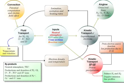
The numerical model TRANS4 is based on two approaches. The first set of codes is TRANSCAR (Lilensten and Blelly, 2002). TRANSCAR is a coupled kinetic/fluid model which solves sequentially the Boltzmann kinetic equation for suprathermal electrons and the Boltzmann momentum equa-tions for N+2, O+2, O+, N+, NO+ and H+ ions between 90
and 3000 km. Each part is linked with the other. The fluid part uses the ionisation and heating rates computed by the kinetic transport code; the kinetic part uses the electron den-sity and temperature computed by the fluid part (Fig. 1). For the ion production, two mechanisms are taken into account.
Fig. 1. Architecture of TRANS4, a multicoupled proto-electron kinetic/fluid transport numerical model.
First, the primary production is the ionisation of the ther-mosphere due to solar EUV (photoproduction) or to electron precipitation. Collisions of primary suprathermal electrons can in turn ionize the neutral gas. Ions and secondary elec-trons are generated. In order to take into account this addi-tional ion production, we use a kinetic transport formalism which describes the 1-D vertical energy degradation of the suprathermal electrons in the ionosphere. This formalism constitutes the kinetic part of TRANSCAR (Lummerzheim and Lilensten, 1994).
The second set of equations describes the kinetic transport of (H+,H) particles. It is described in Galand et al. (1997,
1998) who solved for the first time the dissipative proton-hydrogen kinetic Boltzmann equation. The resolution con-sists of an analytical solution of the coupled (H+,H) system,
with the introduction of dissipative forces. It introduces a continuous loss function as an additional external force so that the set of coupled equations takes the form of a sparse matrix to invert. This code has been successfully tested using experiments (Lilensten and Galand, 1998). The computation of the hydrogen Balmer profiles uses the cross sections given by Basu et al. (1987) (excitation and ionisation cross sec-tions), Kozelov and Ivanov (1992) (elastic cross secsec-tions), van Zyl and Neumann (1980) and Yousif et al. (1986) (emis-sion Hα and Hβcross sections through collisions of (H, H+)
with N2, O2and O). The angular redistribution encountered
by hydrogen particles is described by a phase function. In the following, we will study the effect of several theoretical for-mulations of this function (Rutherford or Maxwellian distri-bution). The Rutherford phase function for protons, equal to the Rutherford formula used for electrons (Stamnes, 1980),
is centered on the pitch angle of the incoming particle and is controlled by a screening parameter equal to 1×10⁻³in the
case of protons (Galand et al., 1998).
The two parts (kinetic proton on one hand, kinetic electron and fluid on the other hand) have always been run indepen-dently, introducing two kinds of inaccuracies. The first and minor one is simply due to the transfer of parameters through independent files. The second one is trickier. As any time-dependent code, this one needs to reach an equilibrium be-fore the results may be reliable. When the codes are run inde-pendently, the equilibrium is reached by running the kinetic transport of the electrons only (TRANSCAR code). The pro-ton precipitation effects are then added to the system. When all the transports are considered simultaneously (TRANS4 code), the effects of the protons on the electron density are taken into account even during the starting phase. The dis-crepancy between the independent method and the integrated one can reach 5 percent on the final electron density.
2 Application to a geophysical event using the ESR, DMSP and optics: 22 January 2004
2.1 General description
We chose as a case study the 22 January 2004. An exten-sive overview of this geophysical event is given by Lorentzen et al. (2007). The period of interest spans within half an hour about 08:45 UT at Svalbard, Norway (78◦N, 16◦E).
Multiple instruments were observing the ionosphere simul-taneously. This study was set up for the Svalbard EISCAT Rocket Study of Ion Outflows (SERSIO) rocket experiment
Fig. 2. Differential particle fluxes in units of cm−2s−1eV−1
ver-sus energy (in keV) and averaged over 30 s between 08:44:55 and 08:45:25 UT as measured by DMSP. Black circles represent the par-ticle electron flux distribution and black triangles the proton flux distribution. Though the proton fluxes at their peak are nearly 100 times less intense, their average energy is twice as high, i.e. 1 keV vs. 400 eV for the electrons. Each spectrum is extrapolated at high and low energies (solid and dashed lines for electrons and protons respectively), where they show a behaviour very different from a Maxwellian distribution.
contributed by Dartmouth College, Cornell University, Uni-versities of Oslo and Svalbard (UNIS), Nagoya University, University of Southampton and University of Leicester. The rocket was launched at 08:57 UT, roughly 10 min after a DMSP satellite pass. Therefore the rocket results will not be considered here. This day was one of the most active in January 2004. Two C-class CMEs, hurled into space near sunspot 540 in the Earth’s direction, were observed by SOHO in less than 48 h prior to the measurements. A stream of fast solar wind (∼700 km s−1) then led to a geomagnetic
storm which began to develop at 01:30 UT on 22 January 2004 (strong Bz>0 of ∼20 nT). Near the L1 point in the
solar wind upstream of the Earth, between 00:00 UT and 10:00 UT, the ACE spacecraft (Chiu et al., 1998), showed in-terplanetary magnetic field conditions typical of lobe recon-nection configurations, with Bz mostly positive and strong
By<0, which lasted for the entire period considered here.
According to ACE, the CME reached the spacecraft around 01:00 UT, when the solar wind velocity jumped from 450 to nearly 700 km s−1. For such a velocity, there is a time
delay of 45 min from ACE to the Earth’s magnetopause. Several Bz-negative episodes appeared between 05:00 and
08:00 UT, lasting half an hour on average, which were corre-lated with variations in the ground-based magnetograms. At 08:00 UT, a strong Bz-negative flow was recorded by ACE,
which was responsible for the strong perturbation of the ge-omagnetic field seen in the Longyearbyen magnetogram one
hour later. At the same time, all-sky cameras and spectrome-ters recorded large enhancements indicative of enhanced pre-cipitation fluxes. The 630.0 nm red and 557.7 nm green emis-sion line intensities increased by factors up to 3, a tendency observed as well for Hαspectra.
The ground-based magnetograms, recorded at Longyear-byen, Ny- ˚Alesund and Tromsø, and maintained at the Tromsø Geophysical Observatory, showed very sharp vari-ations of all three magnetic components from 01:30 UT throughout the day with a very rapid variation around 09:00 UT. The decimetric solar index F10.7 was 130. The
magnetic planetary index showed important variations over a few days before the event, and culminated in Ap=130 at 09:00 UT with a daily average of 60. Because the event was during the winter with a solar zenith angle of χ =98◦, hardly
any photoionisation was present. 2.2 Ionospheric measurements 2.2.1 DMSP F13 data
The Defense Meteorological Satellite Program (DMSP) op-erated by the Air Force is a programme involving numer-ous spacecraft orbiting the Earth since the 1960s in Sun-synchronous near-polar orbits. DMSP F13 was launched in 1995 in a 800 km-altitude orbit and carries among other in-struments a precipitating electron and ion spectrometer SSJ/4 sampling the range 30 eV–30 keV. DMSP F13 closest ap-proach to the ESR 32 m beam was at 08:45:10 UT. The coor-dinates of the spacecraft were geographic latitude 77.5◦and
longitude 9.4◦, i.e. more than 6◦in longitude away from the
ESR location, corresponding to roughly 150 km at this lati-tude when projected to an altilati-tude of 100 km. Therefore the DMSP precipitating fluxes are not an exact measurement of the situation right over the ESR.
The proton fluxes were averaged over 30 s centred on 08:45:10 UT (Fig. 2) and extrapolated at low energies, i.e. below 30 eV. Below 30 eV, the shape of the electron spectrum is becoming strongly non-Maxwellian. We use here a shape for the extrapolation increasing slowly with the decreasing energies (of the form α e−γ)to reach a second maximum at 1 eV, a curve shape corroborated by satellite and rocket mea-surements (Hardy et al., 1985; Winningham and Heikkila, 1974). This average over 30 s was also applied to the elec-tron distribution for the sake of consistency. Numerically, we reach an equilibrium in TRANS4 by introducing a constant precipitation throughout the run and not by turning it on and off again in a short time.
Two peaks are present in the electron flux distribution, the largest one at very low energies (<10 eV nearly reaching 108cm−2s−1eV−1), the other centred around 400 eV
reach-ing 2×106cm−2s−1eV−1. According to the model, above
10 keV, the flux of precipitating particles is too small to con-tribute significantly to the ionisation.
2.2.2 ESR and optical observations
The EISCAT Svalbard Radar (ESR) is situated at (78.15◦N,
16.03◦E) geographic coordinates. The ESR facility is
com-posed of two antennae, one fixed dish 42 m in diameter and aligned along the B-field, the other antenna being steerable and 32 m in diameter. In the following study, only the 32-m antenna is used. The original data recorded by the ESR run on 22 January 2004 show multiple occurrences of natu-rally enhanced ion acoustic lines which corrupt the standard EISCAT analysis (using the GUISDAP software) in the top-side ionosphere. The ESR data were therefore reprocessed with a technique expounded in Ogawa et al. (2000, 2006). It is also known that ion composition and collision frequency models have high influences on the output parameters, in particular ion and electron temperatures below 300 km alti-tude. We therefore used ion and electron temperatures above 300 km for quantitative comparison between data and model. The 32-m steerable dish was pointed at 70.8◦ elevation to
the west (azimuth 261.1◦) of Longyearbyen. The
coordina-tion period is preceding a much more active one where elec-tron densities gradually build up to 1011m−3 with a main
peak situated around 300 km. At the coordination time span, the e−and ion temperatures are significantly high, with very
high ion temperature recorded around 400 km (Ti∼3000 K)
in comparison to the electron temperature (Te∼2000 K at the
same altitude). High Ti can be interpreted as an evidence
for the presence of strong electric fields in the lower iono-sphere through frictional heating (see the review of Brekke and Kamide, 1996). These electric fields are taken into ac-count in our modelling.
2.2.3 The Ebert-Fastie spectrometer data: the Hα and Hβ
lines
Two Ebert-Fastie spectrometers were running at the time of the coordination, one located at Nordlysstasjonen (Advent-dalen) near Longyearbyen, called Green, and the other sit-uated at Ny- ˚Alesund called Black (Holmes et al., 20071). The focal length of the Green spectrometer is 1 m and it measures the auroral Hβ line (486.1 nm). The Black
spec-trometer, of focal length 0.5 m, is calibrated for the Hα line
(656.3 nm). The Full Width at Half Maximum (FWHM) of the instruments spans from 4.2 ˚A (Black) to 3.1 ˚A (Green). Unfortunately, at the time of the coordination with DMSP, the sky was covered with a thin cloud layer, which smeared out the observed spectral lines. Moreover, the presence of a cloud cover precludes the possibility of comparing directly the measured and modelled intensities. The Hαspectra have
been averaged over 2 cycles of 1 min each in order to improve the signal-to-noise ratio. At around 6560 ˚A, a broad peak
cor-1Holmes, J. M., Kozelov, B., Sigernes, F., Lorentzen, D. A.,
and Deehr, C. S.: Dual site observations of dayside Doppler-shifted hydrogen profiles: preliminary results, Can. J. Phys., submitted, 2007.
responding to the Hαline is seen, indicating a slight Doppler
blue shift in the peak of 2 ˚A at the most, i.e. a line-of-sight velocity of 100 km s−1. This shift is weak in comparison to
commonly observed blue shifts which can reach 500 km s−1
(Søraas et al., 1994). This low value is an indication of soft-energy proton precipitation. Moreover an important red shift can be seen, its half width extending 7 ˚A from the centred wavelength λ0 towards smaller wavelengths. This red shift
cannot be attributed only to instrumental broadening. As the 630.0 nm red line, routinely used to calibrate the spectra, is situated spectroscopically far away from the Hα
line it is sometimes better to recalibrate manually the spec-trum around 6500 ˚A through OH(6-1) rotational bands which show features at 6500, 6580 and 6600 ˚A. The OH contribu-tion has been subtracted from the Hα line in the processed
data by using a modelled OH spectrum based on Sigernes et al. (2003) and described in Holmes et al. (2007)1. Be-cause of scattered sunlight approaching local noon, the Hβ
profiles obtained were superimposed on a background con-taining significant Fraunhofer absorption near the Hβ rest
wavelength. Although methods currently exist to account for this twilight component of the background (Robertson et al., 2006; Borovkov et al., 2005), the profiles were not chosen for analysis.
2.3 Comparison between measurements and computations 2.3.1 Optical data: modelled parameterization of the
im-pact of protons
Hαand Hβ integrated zenith spectral profiles
We investigate here the effects of the angular redistributions on the overall shape of the spectral lines. Several cases are studied, involving no angular redistributions, magnetic mir-roring effects, angular redistributions due to elastic scatter-ing, and combined magnetic/collisional angular redistribu-tions. Angular redistributions will affect the red-shifted part of the spectrum, while the blue-shifted peak position will be unchanged, because it arises only from downward (H+,H)
fluxes. However the peak intensities will change according to the upward supplementary contribution involved, observ-ing a slight decrease as the impact of angular redistributions becomes more important. In the event we are studying, we expect the collisions to play an important role since the ener-gies involved in the main precipitation are low. This sensitiv-ity aspect was already pointed out in previous works, either experimental (Gao et al., 1990) or theoretical (Basu et al., 1993; Galand et al., 1998). Laboratory measurements on dif-ferential cross sections have shown the energy dependence of angular redistributions as well (Fleischmann et al., 1967; Newman et al., 1986). The flexibility that the model allows concerning these parameters is investigated through the use of different angular redistribution functions (Maxwellian dis-tribution and Rutherford cross section) for charge-changing
reactions and elastic scattering. The magnetic mirroring is-sue is also addressed, though its contribution is expected to be weak for incoming proton fluxes with an isotropic angular distribution, which is assumed to be the case here (see the early work of Bagariatskii (1958a, b) and the recent confir-mation of Galand et al., 1998). At a given pitch angle a par-ticle of lower energy will correspond to a smaller Doppler shift.
The input proton fluxes are taken from DMSP at 08:45 UT on 22 January 2004. They have an average energy of 1 keV with a flux of 1.5 erg cm−2s−1, i.e. 9.34×10¹¹eV cm−2s−1.
The neutral atmosphere is given by the model MSIS-90 (Hedin, 1991) and O densities are divided by 2 to be more representative of a high latitude thermosphere (Lilensten et al., 1996).
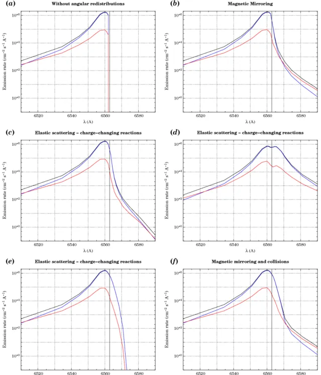
Without angular redistributions
The spectrum, plotted in Fig. 3a, is simple: no red shift is observed, while the blue shift peak is situated around 2.8 ˚A short of the centred line with an intensity reaching 2×106cm−2s−1A˚−1. This blue shift corresponds to a
par-allel velocity of 127 km s−1, which is very slow in
compari-son to Doppler shifts commonly measured in proton events, reaching velocities up to three times as large (e.g. Søraas et al., 1974; Lanchester et al., 2003). This first result is consis-tent with the spectral shifts recorded from the ground in
Ny-˚
Alesund. Incoming protons of low mean energies (∼1 keV) precipitating in the topside ionosphere are responsible for such slight Doppler shifts, as already shown by the DMSP differential particle fluxes.
As the proton fluxes are contributing on average less than the hydrogen fluxes to the overall emission rate, they are only responsible for 5% of the total emission rate at the peak around 6560 ˚A. However this tendency reduces at large Doppler shifts (30 ˚A) where the proton fluxes become larger than the hydrogen ones, resulting in a majority contribu-tion of precipitating H+ that have then been neutralized.
This phenomenon comes intrinsically from the distribution of equilibrium charge fractions for H+ and H, which states
the proportion of each charge state as a function of energy. They are simply expressed as the ratio between electron cap-ture cross sections (respectively ionization-stripping) and the total charge-changing collision cross section for each species N2, O2 or O (see e.g. Rees, 1982). At low energy,
hydro-gen atoms will dominate the composition, while protons will be the major species above a few tens of keV. This prelimi-nary statement will be examined in more details in the case of collisional angular redistributions.
Impact of magnetic mirroring on spectral line profiles and altitude of mirror point
The magnetic mirroring effect, by reflecting charged parti-cles upwards produces a red-shifted tail in the spectral
distri-bution (Fig. 3b). The computed intensity drops sharply near the centred wavelength (around 103cm−2s−1A˚−1). If fitted
by a bi-Gaussian-type distribution following the method ex-plained in Lummerzheim and Galand (2001), the full width at half maximum on the red side reaches 2 ˚A, a value in-side the instrumental broadening, while on the blue in-side, it reaches 10 ˚A. When we look at the spectra recorded at
Ny-˚
Alesund for this event, we can see clearly the red wing of the line, which is almost symmetric with a 9- ˚A wide red tail at half maximum. This confirms that the magnetic mirroring cannot explain solely the shapes observed for the Hα line.
This outcome is to be linked to the region where the mag-netic mirroring becomes effective; it mainly acts at higher al-titudes, converting particles having high pitch angles to parti-cles with lower pitch angles, hence the change of slope in the spectral distribution on the red side (Lorentzen et al., 1998; Kozelov, 1993). The upward fluxes are generated by mag-netic mirroring at higher altitudes, typically in the upper F1
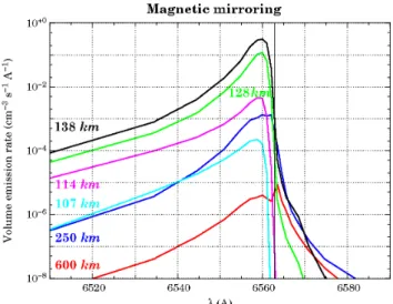
region, and, for 10 keV protons, are well above the energy deposition region usually situated between 110 and 130 km, where the main blue-shifted peak of the Balmer lines occurs induced by downward fluxes. In our case, the mean ener-gies involved are much smaller (1 keV with a large high en-ergy tail as shown in the DMSP data) and the enen-ergy depo-sition peak occurs between 140 and 150 km, making it more sensitive to magnetic mirroring effects. For an isotropic ini-tial distribution, the penetration depth for 1 keV protons pre-cipitating into the ionosphere is typically around 150 km, which coincides with the altitude computed by TRANS4 where magnetic mirroring begins to act. The effect of up-ward fluxes arising from magnetic reflection becomes sig-nificant at the deposition peak and makes the red-shifted tail grow with increasing altitude (Fig. 4). From 140 km up to 600 km the magnetic mirroring populates preferen-tially the longer wavelengths, and the volume emission rate reaches 10−7cm−3s−1A˚−1at 6570 ˚A. In comparison, at the
same Doppler shift the volume emission rate at 128 km drops to 10−8cm−3s−1A˚−1, while it becomes completely
negligi-ble at lower altitudes due to the complete energy degradation of proton fluxes at these altitudes.
With increasing altitude, two peaks on either side of λ0are
appearing. For 90◦pitch-angles, i.e. near λ
0, both high and
low energies contribute to the emission rates. But, when the altitude increases, so do the high energy fluxes, which be-come predominant over the low-energy ones above 200 km. These high-energy fluxes are responsible for an overall en-hancement of the emission, a raise particularly visible near λ0where in contrast only low-energy fluxes contribute to the
emission rates, producing a sudden drop in intensity. We must also notice that high red shifts are created by high-energy particles having small pitch angles, a consequence of the propagation of upward fluxes in the upper part of the ionosphere. However, to account for more symmetric shapes of the observed spectral line which the magnetic mirroring cannot explain, we will now study the effect of collisions on
Fig. 3. Hα spectra computed by TRANS4 with initial DMSP proton fluxes, drawn together with the centred wavelength λ0=6562.8 ˚A. The
overall integrated emission rate is shown in black, and the contribution from the hydrogen flux and the proton fluxes are shown in blue and red, respectively. In panel (a), the results without angular redistributions of magnetic or collisional origins are shown. Only a 3- ˚A blue-shifted peak is seen. Panel (b): with magnetic mirroring, a narrow red-blue-shifted tail appears which extends to a few ˚Angstr¨oms off the centred wavelength. Panels (c) and (d): collisional angular redistributions make the line more symmetric. Here different configurations are shown for both phase functions of elastic and charge-changing scattering: Maxwellian distributions with successively σ =0.05 (c) and σ =0.20 (d), and the more accurate approach of Rutherford (e). The spreading of the line with increasing angular scattering is clearly visible. Panel (f): combined contributions for magnetic mirroring effects and elastic scattering using Rutherford formula.
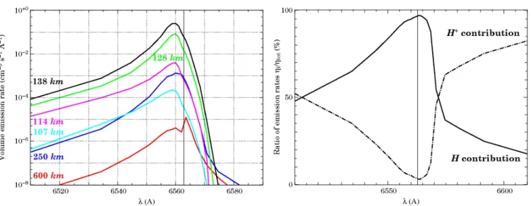
Fig. 4. Hα volume emission rates in cm−3 s−1A˚−1computed by TRANS4 with magnetic mirroring at 107 km (cyan), 114 km (ma-genta), 128 km (green), 138 km (black), 250 km (blue) and 600 km (red). The effective maximum emission is encountered at around 140 km, which is consistent with particles of mean energy ranging between 1 and 2 keV. Only magnetic mirroring effects are consid-ered here.
the overall shape of the lines, as shown in Fig. 3.
Study of collisions for charge-changing and elastic collision reactions
A few cases have been considered which are shown in Fig. 3c and d in order to show the influence of collisional angu-lar redistributions on the shape of spectral lines, which will serve as groundwork for the comparison between data and the model in Sect. 1.3. Not surprisingly, the shape of the lines can become dramatically sensitive to collisional redis-tributions, playing a larger role than magnetic mirroring. A real modulation of the red-shifted part can be performed and is very much dependent on the phase functions chosen to ac-count for this mechanism. A Maxwellian distribution with a standard statistical deviation σ ranging between 5% and 20% was first chosen and the results are shown in Figs. 3c and d. The red-shifted tail broadens significantly between the two cases, from 2 ˚A to 7 ˚A, a value that approximates the blue-shifted part of the line. For σ =5% on Fig. 3c, the full width at half maximum of the right side of the spectrum is comparable to that of the mirroring effect, i.e. 1 to 2 ˚A. In comparison, this value can extend up to 8 ˚A in the extreme case of a Maxwellian distribution of σ =20% (Fig. 3d), which indicates that when choosing a wide angular redistribution due to collisions, computed Doppler shifts can become con-sistent with the measurements. Compared to magnetic mir-roring, collisional angular redistributions play the major role at least at low Doppler shifts in the creation of the observed spectrum, a conclusion that was previously put forward to
ac-Fig. 5. Hα emission rate Doppler profile computed for collisional angular redistributions applied successively below 1 keV (solid line) and below 10 keV (dashed line). The Rutherford formula is used. One can see the red wing extend significantly in amplitude when angular redistributions below a higher threshold are included.
count for Hβ lines (Lanchester et al., 2003). In this case, the
line can become completely symmetric with a second peak appearing at longer wavelengths near 6565 ˚A. This is an in-dication that strong fluxes are generated by particles having frequently changed pitch-angles and energies because of the increasing number of collisions at low altitudes, while at λ0,
only a few particles remain unchanged.
The angular redistribution due to collisions appears to make the fluxes more isotropic in the lower ionosphere, while at high altitudes, changes in pitch angles and energy occur less often because of the decreasing atmospheric density. Soft protons are more likely to be sensitive to collisions; hence the choice of the phase function is a crucial issue. If we increase the number of angles accessible for a given incoming particle colliding with a neutral species, both proton and hydrogen upward fluxes generated will be strongly enhanced, especially since collision cross sections (and charge-changing reaction cross sections even more so) remain high under 10 keV. Forward scattering is assumed for particles having energies above 1 keV, but this limit might be increased to higher energies depending on the event chosen. This physical limit will modulate the extent of the red wing to higher energies as shown in Fig. 5 for a threshold of 10 keV instead. The blue part of the spectrum is unchanged but the red wing is more raised which confirms the sensitivity of the results to the Rutherford parameter. Including redistributions at high energies can have a dra-matic effect and may change the position of the peak in the case of high-energy proton precipitation. This was already emphasized in Lanchester et al. (2003) in the case of Hβ,
Combined effects and detail of the impact of (H, H+) fluxes on the overall distribution
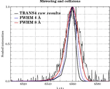
We now compare the spectral Hαdata with the model outputs
including magnetic mirroring and Rutherford collisional an-gular redistributions. These results are shown in Fig. 6. To take into account the spectrometer’s resolution, the profiles produced by the models are convolved with the instrumental function which is taken as a triangle function with different widths at half maximum, spanning from the nominal FWHM (around 4 ˚A) to larger values (8 ˚A). Generally, the geometry of the entrance and exit slits of an Ebert-Fastie spectrome-ter produces a trapezoidal instrumental function. When the widths of both of the slits are matched, the function becomes triangular (Lerner and Thevenon, 1988). By degrading ar-tificially the resolution of the instrument, we show that the model can reproduce the measurements very well. In Fig. 6, we present the first comparison between the model, drawn in black solid line, including angular redistributions (magnetic mirroring and Rutherford scattering applied below 1 keV) and the spectral intensity recorded by the Black spectrom-eter (noisy curve). The narrow nominal profile of the spec-trometer cannot explain by itself the differences observed, and we have to increase substantially the width of the instru-mental function to get profiles similar to those recorded by the instrument. We have degraded the resolution of the in-strument, which can be interpreted as an estimate of the thin cloud-coverage on the hydrogen lines or an inaccurate origi-nal determination of the instrumental bandpass.
The main results of this approach are shown in Fig. 7, where emission rates and volume emission rates for given altitudes are plotted. Magnetic mirroring becomes impor-tant at higher altitudes and is particularly significant at high Doppler shifts, while the angular distributions due to elas-tic and charge-changing reactions reach their full power at lower altitudes and for red shifts between 1 and 8 ˚A. The ra-tios of emission rates drawn in Fig. 7 (right) illustrate this double impact and can be seen as a mix of magnetic and col-lisional redistributions. The red wing reveals a greater impact of hydrogen atoms at smaller red shifts as in the Rutherford scattering case. For spectral shifts to longer wavelengths, the protons play the major role in the emission, matching the conclusions that were drawn in the magnetic mirroring case.
Results for Hβ
Following the validation of our approach in terms of angu-lar redistributions and spectral widths, we show in Fig. 8 the emission rates expressed in cm−2s−1A˚−1for H
β. The
over-all intensity is smover-aller than for Hα by a factor 2, which is
consistent with the preliminary modelling of Galand (1996) and Galand et al. (2004). Both collisions and magnetic
mir-Fig. 6. First out-of-the-box comparison between spectral Hα data recorded at Ny- ˚Alesund (discontinuous line) and the model (black line). A triangle function of FWHM=4 ˚A was first chosen for the in-strumental function, which was then convolved with the raw results from the model. The resulting intensity is drawn in blue. When us-ing a triangle function of FWHM=8 ˚A, the model yields the result-ing line intensity drawn in red, which matches the measurements quite well.
roring are easily seen, the former at smaller red shifts the latter at bigger red shifts.
2.3.2 Comparison to radar data and validation of the ap-proach
ESR measurements
Figure 9 shows the electron density height profiles produced by the model in the case of combined electron-proton pre-cipitation versus the electron densities recorded by ESR aver-aged here over 20 min. This mean value is then representative of the ionospheric conditions around the coordination time at 08:45 UT while the DMSP satellite was at 800 km. The ESR error bars are drawn at altitudes higher than 300 km.
The temperatures (not shown here) exhibit a typical electric-field event behaviour. The ion temperature reaches a value of 3000 K at 400 km which is larger than the elec-tron temperature (2000 K). This effect implies modifications in the ion composition around the F1 layer (Lathuill`ere and Kofman, 2006), which makes it meaningless to compare the IS temperatures with TRANS4 outputs. However, the elec-tron densities are deduced from fitting of the incoherent scat-ter spectrum and are thus useable for our comparison. Ion ve-locities obtained by the ESR 32-m dish were −600 m s−1at
220 km altitude at 08:45 UT. The high ion velocity indicates that a strong eastward flow at a speed of 1500 m s−1occurred
Fig. 7. Hα spectra yielded by TRANS4 when taking into account angular redistributions of both magnetic and collisional origins under Rutherford’s approximation for the phase function. The left panel is the detail of altitude contributions to the total volume emission rate. The same colour code as in Fig. 4 is used: 107 km (cyan), 114 km (magenta), 128 km (green), 138 km (black), 250 km (blue) and 600 km (red). In the right panel, the ratio of the contributions of proton (dash-dot) and hydrogen (solid line) to the total Hαemission rate is plotted.
Fig. 8. Hβemission rates including angular redistributions of mag-netic and collisional origins. In blue the hydrogen contribution to the emission is plotted, and in red the proton contribution.
the ESR measurements correspond to a first estimate of the electric field of 60–80 mV/m (not shown here). When com-paring the direct model outputs with the incoherent scatter temperature, it results in a more accurate value of 65 mV/m, which was used in the density computations. Because of the strong electric field encountered, we expect an electron den-sity depletion in the F region ionosphere compared to the case where no electric field is present, and the effect is also included in the model.
Fig. 9. Contribution of precipitating electrons (dash line) as a single
source in the code and of proton precipitation (dash-dotted line) as a single source in the code to the total electron density (black solid line). The model’s outputs are drawn versus the ESR averaged mea-sured electron densities, which are indicated with black triangles.
Though below 250 km the computed densities are larger than the measured densities by a factor three, a perfect match is found between 300 and 800 km. This difference is no surprise. As emphasized in the description of the data (Sect. 2.2), we expect the model to be accurate in the range 600–800 km. The electron and proton fluxes recorded by
DMSP are indeed representative of the region probed by EIS-CAT at these altitudes at the coordination time. However, in the first few hundred kilometres along the ESR 32-m beam, we are geographically and magnetically far from the condi-tions traversed by the satellite. The condicondi-tions were very dif-ferent from one probed region to another. In the all-sky cam-era images (not shown here, see Simon, 2006, or Lorentzen et al., 2007), the region probed at 100 km by the ESR beam was less active than the upper regions which were also fur-ther away from the radar site in the horizontal direction. This is also confirmed by the model and, as shown in Fig. 9, a fac-tor of three in electron densities is required at low altitudes to account for the data.
In the same plot, we show an estimate of the electron den-sities due to the two sources. In one run, we turn on only the electron precipitation and in a second run only the proton pre-cipitation. Although the system is not totally linear because of the chemistry and fluid transport, this gives an idea of the contribution of each source. In particular, it shows that the proton precipitation is responsible for the electron densities at low altitudes (around 110 km) while the electron precipi-tation creates electron densities at altitudes above 170 km.
3 Conclusion
This work presents the first coupled numerical ionospheric code that dynamically solves the fluid, electron and proton kinetic equations. It allows retrieving macroscopic parame-ters such as the electron density or Balmer hydrogen emis-sion lines as well as microscopic parameters such as the dis-tribution function and electron fluxes. We have shown the results compared to a set of experimental data during a co-ordinated experiment (DMSP, ESR, spectrometer and all-sky cameras) situated in the cusp region. This allowed us to show the respective effects of collisions and magnetic mirroring on the transport of precipitating protons. We also showed that, in this event, protons were responsible for the low-altitude density peak and contributed up to 15% of the total ionisa-tion above an altitude of 200 km.
Acknowledgements. C. Simon would like to thank D. Lorentzen
(University Centre on Svalbard UNIS, Norway) and F. Pitout (LPG, France) for their fruitful comments and discussions throughout the preparing of this work and the interpretation of data. The authors thank H. Opgenoorth (ESA ESTEC, the Netherlands) for his con-structive advices on the original manuscript. We would like also to thank C. Deehr of the Geophysical Institute for having made avail-able the 0.5 m Black spectrometer data and F. Sigernes (UNIS) who operated and maintained the instrument during the campaign 2003– 2004. We are indebted to the director and staff of EISCAT for op-erating the facility and supplying the data. EISCAT is an Interna-tional Association supported by Finland (SA), France (CNRS), Ger-many (MPG), Japan (NIPR), Norway (NFR), Sweden (NFR) and the United Kingdom (PPARC). Financial support has been provided by the Norwegian Research Council and AFOSR task 2311A5.
Topical Editor M. Pinnock thanks two referees for their help in evaluating this paper.
References
Bagariatskii, B. A.: The Influence of Proton Spiral Trajectories on the Doppler Profile of Auroral Hydrogen Lines, Sov. Astron., 2, 87–96, 1958a.
Bagariatskii, B. A.: The Zenith Angle Distribution Function of Au-roral Protons, Sov. Astron., 2, 453, 1958b.
Basu, B., Jasperse, J. R., Robinson, R. M., Vondrak, R. R., and Evans, D. S.: Linear transport theory of auroral proton precipi-tation – A comparison with observations, J. Geophys. Res., 92, 5920–5932, 1987.
Basu, B., Jasperse, J. R., and Grossbard, N. J.: A numerical solution of the coupled proton-H atom transport equations for the proton aurora, J. Geophys. Res., 95, 19 069–19 078, 1990.
Basu, B., Jasperse, J. R., Strickland, D. J., and Daniell Jr., R. E.: Transport-theoretic model for the electron-proton-hydrogen atom aurora. 1: Theory, J. Geophys. Res., 98, 21 517– 21 532, 1993.
Borovkov, L. P., Kozelov, B. V., Yevlashin, L. S., and Chernouss, S. A.: Variations of auroral hydrogen emission near substorm onset, Ann. Geophys., 23, 1623–1635, 2005,
http://www.ann-geophys.net/23/1623/2005/.
Brekke, A. and Kamide, Y.: On the relationship between Joule and frictional heating in the polar ionosphere, J. Atmos. Terr. Phys., 58, 139–143, 1996.
Chakrabarti, S., Pallamraju, D., Baumgardner, J., and Vaillancourt, J.: HiTIES: A high throughput imaging echelle spectrograph for ground-based visible airglow and auroral studies, J. Geophys. Res., 106, 30 337–30 348, doi:10.1029/2001JA001105, 2001. Chamberlain, J. W.: The Excitation of Hydrogen in Aurorae.,
As-trophys. J., 120, 360–366, 1954a.
Chamberlain, J. W.: On the Production of Auroral Arcs by Incident Protons., Astrophys. J., 120, 566–571, 1954b.
Chamberlain, J. W.: On a Possible Velocity Dispersion of Auroral Protons., Astrophys. J., 126, 245–252, 1957.
Chiu, M. C., von-Mehlem, U. I., Willey, C. E., Betenbaugh, T. M., Maynard, J. J., Krein, J. A., Conde, R. F., Gray, W. T., Hunt Jr., J. W., Mosher, L. E., McCullough, M. G., Panneton, P. E., Staiger, J. P., and Rodberg, E. H.: ACE Spacecraft, Space Sci. Rev., 86, 257–284, doi:10.1023/A:1005002013459, 1998. Davidson, G. T.: Expected Spatial Distribution of Low-Energy
Pro-tons Precipitated in the Auroral Zones, J. Geophys. Res., 70, 1061–1068, 1965.
Deehr, C. S., Lorentzen, D. A., Sigernes, F., and Smith, R. W.: Dayside auroral hydrogen emission as an aeronomic signature of magnetospheric boundary layer processes, Geophys. Res. Lett., 25, 2111–2114, doi:10.1029/98GL01535, 1998.
Eather, R. H.: Red Shift of Auroral Hydrogen Profiles, J. Geophys. Res., 71, 5027–5032, 1966.
Eather, R. H.: Secondary Processes in Proton Auroras, J. Geophys. Res., 72, 1481, 1967a.
Eather, R. H.: Auroral proton precipitation and hydrogen emissions, Rev. Geophys., 5, 207–285, 1967b.
Eather, R. H. and Burrows, K. M.: Excitation and ionization by auroral protons, Aust. J. Phys., 19, 309–322, 1966.
Eather, R. H. and Jacka, F.: Auroral hydrogen emission, Aust. J. Phys., 19, 241–274, 1966.
Edgar, B. C., Miles, W. T., and Green, A. E. S.: Energy deposi-tion of protons in molecular nitrogen and applicadeposi-tions to proton auroral phenomena, J. Geophys. Res., 78, 6595–6606, 1973. Edgar, B. C., Porter, H. S., and Green, A. E. S.: Proton
en-ergy deposition in molecular and atomic oxygen and appli-cations to the polar cap, Planet. Space Sci., 23, 787–804, doi:10.1016/0032-0633(75)90015-X, 1975.
Fang, X., Liemohn, M. W., Kozyra, J. U., and Solomon, S. C.: Quantification of the spreading effect of auroral proton pre-cipitation, J. Geophys. Res. – Space Physics, 109, A04309, doi:10.1029/2003JA010119, 2004.
Fleischmann, H. H., Young, R. A., and McGowan, J. W.: Differen-tial Charge-Transfer Cross Section for Collisions of H+on O2,
Phys. Rev., 153, 19–22, doi:10.1103/PhysRev.153.19, 1967. Galand, M.: Transport des protons dans l’ionosph`ere aurorale,
Th`ese de l’Universit´e Joseph Fourier, Grenoble, 1996.
Galand, M.: Introduction to special section: Proton precip-itation into the atmosphere, J. Geophys. Res., 106, 1–6, doi:10.1029/2000JA002015, 2001.
Galand, M. and Chakrabarti, S.: Proton aurora observed from the ground, J. Atmos. Terr. Phys., 68, 1488–1501, doi:10.1016/j.jastp.2005.04.013, 2006.
Galand, M., Lilensten, J., Kofman, W., and Sidje, R. B.: Proton transport model in the ionosphere 1. Multistream approach of the transport equations, J. Geophys. Res., 102, 22 261–22 272, doi:10.1029/97JA01903, 1997.
Galand, M., Lilensten, J., Kofman, W., and Lummerzheim, D.: Pro-ton transport model in the ionosphere. 2. Influence of magnetic mirroring and collisions on the angular redistribution in a proton beam, Ann. Geophys., 16, 1308–1321, 1998,
http://www.ann-geophys.net/16/1308/1998/.
Galand, M., Baumgardner, J., Pallamraju, D., Chakrabarti, S., Løvhaug, U. P., Lummerzheim, D., Lanchester, B. S., and Rees, M. H.: Spectral imaging of proton aurora and twilight at Tromsø, Norway, J. Geophys. Res. – Space Physics, 109, A07305, doi:10.1029/2003JA010033, 2004.
Gao, R. S., Johnson, L. K., Hakes, C. L., Smith, K. A., and Stebbings, R. F.: Collisions of kilo-electron-volt H+ and He+ with molecules at small angles – Absolute differential cross sections for charge transfer, Phys. Rev. A, 41, 5929–5933, doi:10.1103/PhysRevA.41.5929, 1990.
Gartlein, C. W.: Auroral spectra showing broad hydrogen lines, Trans. Am. Geophys. Union, 31, 18–20, 1950.
Gartlein, C. W.: Protons and the Aurora, Nature, 167, 277, doi:10.1038/167277a0, 1951a.
Gartlein, C. W.: Protons and the Aurora, Phys. Rev., 81, 463–464, doi:10.1103/PhysRev.81.463.2, 1951b.
Hardy, D. A., Gussenhoven, M. S., and Holeman, E.: A statisti-cal model of auroral electron precipitation, J. Geophys. Res., 90, 4229–4248, 1985.
Hubert, B., G´erard, J. C., Fuselier, S. A., Mende, S. B., and Burch, J. L.: Proton precipitation during transpolar auroral events: Ob-servations with the IMAGE-FUV imagers, J. Geophys. Res. – Space Physics, 109, A06204, doi:10.1029/2003JA010136, 2004. Iglesias, G. and Vondrak, R. R.: Atmospheric spreading of protons
in auroral arcs, J. Geophys. Res., 79, 280–282, 1974.
Jasperse, J. R.: Transport theoretic solutions for the beam-spreading
effect in the proton-hydrogen aurora, Geophys. Res. Lett., 24, 1415–1418, doi:10.1029/97GL01271, 1997.
Jasperse, J. R. and Basu, B.: Transport theoretic solutions for auro-ral proton and H atom fluxes and related quantities, J. Geophys. Res., 87, 811–822, 1982.
Johnstone, A. D.: The spreading of a proton beam by the atmo-sphere, Planet. Space Sci., 20, 292–297, 1972.
Kozelov, B. V.: Influence of the dipolar magnetic field on transport of proton-H atom fluxes in the atmosphere, Ann. Geophys., 11, 697–704, 1993,
http://www.ann-geophys.net/11/697/1993/.
Kozelov, B. V. and Ivanov, V. E.: Monte Carlo calculation of proton-hydrogen atom transport in N2, Planet. Space Sci., 40, 1503–1511, doi:10.1016/0032-0633(92)90047-R, 1992. Kozelov, B. V. and Ivanov, V. E.: Effective energy loss per
electron-ion pair in proton aurora, Ann. Geophys., 12, 1071–1075, 1994, http://www.ann-geophys.net/12/1071/1994/.
Lanchester, B. S., Galand, M., Robertson, S. C., Rees, M. H., Lum-merzheim, D., Furniss, I., Peticolas, L. M., Frey, H. U., Baum-gardner, J., and Mendillo, M.: High resolution measurements and modeling of auroral hydrogen emission line profiles, Ann. Geo-phys., 21, 1629–1643, 2003,
http://www.ann-geophys.net/21/1629/2003/.
Lathuill`ere, C. and Kofman, W.: A short review on the F1-region ion composition in the auroral and polar ionosphere, Adv. Space Res., 37, 913–918, doi:10.1016/j.asr.2005.12.014, 2006. Lerner, J. M. and Thevenon, A.: The optics of spectroscopy, a
tuto-rial 2.0, Jobin Yvon Optical Systems, Instruments SA, 1988. Lilensten, J. and Blelly, P. L.: The TEC and F2 parameters as tracers
of the ionosphere and thermosphere, J. Atmos. Terr. Phys., 64, 775–793, 2002.
Lilensten, J. and Galand, M.: Proton-electron precipitation effects on the electron production and density above EISCAT (Tromsø) and ESR, Ann. Geophys., 16, 1299–1307, 1998,
http://www.ann-geophys.net/16/1299/1998/.
Lilensten, J., Blelly, P. L., Kofman, W., and Alcayd´e, D.: Auro-ral ionospheric conductivities: a comparison between experiment and modeling, and theoretical f 10.7 -dependent model for EIS-CAT and ESR, Ann. Geophys., 14, 1297–1304, 1996,
http://www.ann-geophys.net/14/1297/1996/.
Lorentzen, D. A.: Latitudinal and longitudinal dispersion of ener-getic auroral protons, Ann. Geophys., 18, 81–89, 2000, http://www.ann-geophys.net/18/81/2000/.
Lorentzen, D. A., Sigernes, F., and Deehr, C. S.: Mod-eling and observations of dayside auroral hydrogen emis-sion Doppler profiles, J. Geophys. Res., 103, 17 479–17 488, doi:10.1029/98JA00885, 1998.
Lorentzen, D. A., Kintner, P. M., Moen, J., Sigernes, F., Oksavik, K., Ogawa, Y., and Holmes, J. M.: Pulsating dayside aurora in relation to ion upflow events during a northward IMF domi-nated by a strongly negative IMF By, J. Geophys. Res., accepted, doi:10.1029/2006JA011757, 2007.
Lummerzheim, D. and Galand, M.: The profile of the hydrogen Hβ emission line in proton aurora, J. Geophys. Res., 106, 23–32, doi:10.1029/2000JA002014, 2001.
Lummerzheim, D. and Lilensten, J.: Electron transport and energy degradation in the ionosphere: Evaluation of the numerical solu-tion, comparison with laboratory experiments and auroral obser-vations, Ann. Geophys., 12, 1039–1051, 1994,
http://www.ann-geophys.net/12/1039/1994/.
Meinel, A. B.: The spectrum of the airglow and the aurora , Reports of Progress in Physics, 14, 121–146, 1951.
Newman, J. H., Chen, Y. S., Smith, K. A., and Stebbings, R. F.: Differential cross sections for scattering of 0.5-, 1.5-, and 5.0-keV hydrogen atoms by He, H2, N2, and O2, J. Geophys. Res., 91, 8947–8954, 1986.
Ogawa, Y., Fujii, R., Buchert, S. C., Nozawa, S., Watanabe, S., and van Eyken, A. P.: Simultaneous EISCAT Svalbard and VHF radar observations of ion upflows at different aspect angles, Geo-phys. Res. Lett., 27, 81–84, doi:10.1029/1999GL010665, 2000. Ogawa, Y., Buchert, S. C., Fujii, R., Nozawa, S., and Forme, F.:
Naturally enhanced ion-acoustic lines at high altitudes, Ann. Geophys., 24, 3351–3364, 2006,
http://www.ann-geophys.net/24/3351/2006/.
Omholt, A.: Characteristics of auroras caused by angular dispersed protons, J. Atmos. Terr. Phys., 9, 18–27, 1956.
Rees, M. H.: On the interaction of auroral protons with the earth’s atmosphere, Planet. Space Sci., 30, 463–472, doi:10.1016/0032-0633(82)90056-3, 1982.
Robertson, S. C., Lanchester, B. S., Galand, M., Lummerzheim, D., Stockton-Chalk, A. B., Aylward, A. D., Furniss, I., and Baum-gardner, J.: First ground-based optical analysis of Hβ Doppler profiles close to local noon in the cusp, Ann. Geophys., 24, 2543– 2552, 2006,
http://www.ann-geophys.net/24/2543/2006/.
Sigernes, F.: Estimation of initial auroral proton energy fluxes from Doppler profiles, J. Atmos. Terr. Phys., 58, 1871–1883, 1996. Sigernes, F., Lorentzen, D. A., Deehr, C. S., and Henriksen, K.:
Calculation of auroral Balmer volume emission height profiles in the upper atmosphere, J. Atmos. Terr. Phys., 56, 503–508, 1994. Sigernes, F., Shumilov, N., Deehr, C. S., Nielsen, K. P., Svenøe, T., and Havnes, O.: Hydroxyl rotational tempera-ture record from the auroral station in Adventdalen, Svalbard (78◦N, 15◦E), J. Geophys. Res. – Space Physics, 108, 3–1, doi:10.1029/2001JA009023, 2003.
Simon, C.: Contribution to the study of energy inputs from solar origin in the ionosphere: doubly-charged ions and proton ki-netic transport – Application to the Earth and Titan, PhD the-sis, Th`ese de l’Universit´e Joseph Fourier, Grenoble, http://tel. archives-ouvertes.fr/tel-00109802, 2006.
Solomon, S. C.: Auroral particle transport using Monte Carlo and hybrid methods, J. Geophys. Res., 106, 107–116, doi:10.1029/2000JA002011, 2001.
Søraas, F. and Aarsnes, K.: Observations of ENA in and near a proton arc, Geophys. Res. Lett., 23, 2959–2962, doi:10.1029/96GL02821, 1996.
Søraas, F., Lindalen, H. R., M˚aseide, K., Egeland, A., Sten, T. A., and Evans, D. S.: Proton precipitation and the Hβ emission in a postbreakup auroral glow, J. Geophys. Res., 79, 1851–1859, 1974.
Søraas, F., Maseide, K., Torheim, P., and Aarsnes, K.: Doppler-shifted auroral H-beta emission: A comparison between obser-vations and calculations, Ann. Geophys., 12, 1052–1064, 1994, http://www.ann-geophys.net/12/1052/1994/.
Stamnes, K.: Analytic approach to auroral electron transport and energy degradation, Planet. Space Sci., 28, 427–441, doi:10.1016/0032-0633(80)90046-X, 1980.
Strickland, D. J., Daniell, Jr., R. E., Jasperse, J. R., and Basu, B.: Transport-theoretic model for the electron-proton-hydrogen atom aurora. 2: Model results, J. Geophys. Res., 98, 21 533– 21 548, 1993.
van Zyl, B. and Neumann, H.: H-alpha and H-beta emission cross sections for low-energy H and H+collisions with N
2and O2, J.
Geophys. Res., 85, 6006–6010, 1980.
Vegard, L.: Hydrogen showers in the auroral region, Nature, 144, 1089–1090, 1939.
Vegard, L.: Emission spectra of night sky and aurora, Report of the Gassiot Committee, The Physical Society London, 1948. Vegard, L. and Tønsberg, E.: Results from auroral spectrograms
obtained at Tromsø observatory during the winters 1941–1942 and 1942–1943, Geophys. Publik., 16, 1–12, 1944.
Winningham, J. D. and Heikkila, W. J.: Polar cap auroral electron fluxes observed with Isis 1, J. Geophys. Res., 79, 949–957, 1974. Yousif, F. B., Geddes, J., and Gilbody, H. B.: Balmer alpha emis-sion in colliemis-sions of H, H(+), H2(+) and H3(+) with N2, O2and H2O, J. Phys. B: At. Mol. Phys., 19, 217–231, 1986.