Design For Assembly:
A Computational Approach to Construct
Interlocking Wooden Frames
By
Alan Song-Ching Tai
Bachelor of Science in Electrical Engineering
National Taiwan University, 2003
Master of Architecture
University of Pennsylvania 2009
Submitted to The Department of Architecture in Partial
Fulfillment of The Requirements for The Degree of
MASTER OF SCIENCE IN ARCHITECTURE STUDIES
AT THE
MASSACHUSETTS INSTITUTE OF TECHNOLOGY
JUNE 2012
@2012 Alan Song-Ching Tai. All rights reserved.
The author hereby grants to MIT permission to reproduce and to distribute publicly paper and electronic copies of this thesis document in whole or
in part in any medium now known or hereafter created
MASSACHUSETTS INSTITUTE OF TECHNOLOGY
ION
iJUN 0
8 2012
LIRARIES
ARC-IV-Signature of Author:
Department of Architecture
May 24, 2012
Certified by:
-V
-Accepted by:
I
Takehiko Nagakura
Associate Professor of Architecture
Design For Assembly:
A Computational Approach to Construct
Interlocking Wooden Frames
By
Alan Song-Ching Tai
Thesis Committee
Takehiko Nagakura
Associate Professor of Architecture
Thesis Advisor
Dennis Shelden
Associate Professor of Practice
Thesis Reader
Design for Assembly:
A Computational Approach to
Construct Interlocking Wooden Frames
by
Alan Song-Ching Tai
Submitted to the Department of Architecture
on May 24, 2012 in Partial Fulfillment of the Requirements for the
Degree of Master of Science in Architecture Studies
ABSTRACT
This thesis explores the computational process of generating and
constructing interlocking frames. Its outcome delivers a sophisticated
software tool that creates a three dimensional interlocking pattern,
analyzes the intersecting conditions between members, and
immediately provides instruction of its assembly sequence in
animated visualization.
An interlocking frame is a system that consists of short members
spanning on a large surface where members lock each other at their
mid-spans by simple notches. Such a system should be designed
with consideration of its assembly sequence, as a static interlocking
form may be described but impossible to assemble in any sequence.
Given a three dimensional digital model of an interlocking frame, the
feasibility of the disassembly sequence can be assessed by analyzing
the geometric contact constraints between each member. The
assembly sequence can then be obtained by reversing the disassembly
sequence, and helps a designer to evaluate different options in the
earlier stage of design.
The proposed tool uses the genetic algorithm and graph searching
algorithms to find optimized notching configurations that guarantee
an assembly sequence. It can analyze various types of assemblies
defined by planar surface contact constraints, and has a potential for
further development into a versatile, automated 4D simulation tool.
Thesis Supervisor: Takehiko Nagakura
Acknowledgement
First of all, I would like to thank my thesis advisor Professor Takehiko
Nagakura for his support and guidance in the thesis.
I would like to thank Professor Dennis Shelden for joining my
committee as a reader during his year on leave.
I would like to thank Professor Patrick Winston for his valuable input
on problem solving techniques. I would also like to thank Professor
Erik Demaine and Marty Demaine for introducing me the world of
wood puzzles.
I want to say thanks to Duks, Rizal, Skylar, Yanni, Dimitris, Masoud
for their discussions that help to shape this thesis.
I would like to thank all my colleagues in the SMarchS program,
Carolina, Carl, Will, Moritz, Sarah, Josh, Theodora, Katia, and
Masoud. You guys are a fantastic group to work with!
Last, I would like to thank Bruce, Iouyu and, most importantly, my
parents for their greatest support. Without your support, it would be
not be possible for me to continue my studies in architecture.
Table of Content
1. Introduction
10
2. Background
12
2.1 Interlocking Frames
2.2 Nail-less Construction: Construction without
Mechanical Fastener
2.3 Interlocking Frames and Reciprocal Frames
2.4 Design For Assembly
3. Geometric Assembly Planning
18
3.1 Non-Directional Blocking Graph (NDBG) and
Directional Blocking Graph (DBG)
3.2 Non-Directional Free Graph (NDFG)
3.3 Six Degrees of Freedom (DOF)
3.4 Strongly Connected Component (SCC)
3.5 Disassembling the Diagonal Burr Puzzle
3.6 Extended Motion
3.7 Assembly Sequencing
4. Designing Interlocking Frames
26
4.1 From 2D grid to 3D interlocking Pattern
4.2 From 2D Interlocking Pattern to 3D
Interlocking Pattern
4.3 Member Placement in 3D
4.4 Fabrication Constraints
4.5 Searching Joint Condition using the Genetic
Algorithm (GA)
4.6 Defining the Fitness Function for GA
4.7 Recursive Genetic Algorithm for Large
Assembly
5. Software Implementation
38
5.1 Pattern Generator
5.2 Joint Generator
5.3 Sequence Player
5.4 Disassembler
6. Conclusion and Contribution
46
7. Bibliography
48
1. Introduction
An interlocking frame is a system that consists of short members
spanning across a large surface. In this system, all the members
are locked by the adjacent members, resulting in an assembly that
is geometrically stable. In the analysis of geometric stability, the
material of each member is totally rigid and deformation is not
allowed. An interlocking frame should always be designed with the
consideration of its assembly sequence. The 3D CAD
(Computer-Aided Design) model usually represents the finished state of assembly
and does not guarantee a valid assembly sequence. By examining the
geometric constraints between members, the free members can be
identified in the assembly. The disassembly sequence can be solved
by recursively examining and removing the free members. Once the
successful disassembly sequence is discovered, the assembly sequence
can then be obtained by reversing the disassembly sequence. The
algorithm for determining the assembly sequence will be visited in
the Geometric Assembly Planning chapter. One of the important
goals of this thesis is to introduce the knowledge of geometric
assembly planning to the field of architecture, encouraging architects
to integrate this knowledge into the design process.
The process of designing interlocking frames involves in transforming
a two dimensional grid pattern into a three dimensional interlocking
pattern on a free-form surface. Members with the desired dimension
will be placed on the three dimensional pattern with respect to
the surface orientation. These members will intersect in the three
dimensional space and each of the intersection result in a joint
between members. These joints require proper notching to ensure
the interlocking behavior between members. Because of the angle
of intersection is different at every joint, every notching geometry
will need to be uniquely defined. The final product is assumed to
be digitally fabricated using a five-axis CNC (computer numerical
control) machine with a flat end milling bit. This assumption
imposes several constraints on the geometry of notching, and limits
the number of possible joint configuration. However, even under
these fabrication constraints, it is still impossible to examine all
configurations due to their large quantity. Therefore, the genetic
algorithm and various tree searching algorithms are deployed
to search for the optimized joint configuration that allow a valid
assembly sequence. The entire process of designing an interlocking
frame will be documented in the Methodology chapter.
A plugin program is implemented in the Rhinoceros 3D software
to perform the required tasks to design an interlocking frame. This
program creates a three dimensional interlocking pattern, analyzes the
intersecting conditions between members, and immediately provides
instruction of its assembly sequence in an animated visualization.
Besides interlocking frames, it can also analyze generic assemblies
defined by planar surface contact constraints. By adding real world
construction parameters, this tool has the potential for further
development into a versatile, automated 4D simulation tool. The
detail of this software program will be documented in the Software
Implementation chapter.
I
W4
2. Background
An interlocking frame is a system that consists of short members
spanning across a large surface. In this system, all the members are
locked by the adjacent members, resulting in an assembly that is
geometrically stable.
The motivation of studying interlocking frames originates from my
interest in "nail-less constructions," which are construction methods
that do not use any glue or fasteners. I am always intrigued by the
homogeneity of the material and the intelligence built into geometry
in such a construction method. Because interlocking frames does
not rely on the friction fit of its material, it allows more tolerance in
fabrication. It is also easier to assemble, disassemble and reassemble.
Because of its interlocking behavior, an interlocking frame should
always be designed with the consideration of its assembly sequence.
This particular constraint leads to the re-evaluation of the digital
design and fabrication process, where the assembly process is often
overlooked by the designer. This thesis hopes to bring the notion of
assemblability to the attention of architects.
2.1 Interlocking Frames
An interlocking frame is a system that consists of short members
spanning across a large surface, where members locks each other by
simple notches. All of the members in this system do not have any
degrees of freedom because of the interlocking geometric constraints.
The more rigorous definition of locking and constrains will be
introduced in chapter three.
Fig.2.1 shows examples of interlocking frames. The image on the
left is a wooden puzzle, and the one on the right is an experimental
structure built in the campus of ETH Zurich. The term, interlocking
frame, is invented in this paper, and does not exist in any reference.
It originates from the name of both families of objects shown in the
examples, which one is an "interlocking" puzzle and the other is a
reciprocal "frame" structure.
Fig. 2.1
2.2 Nail-less Construction: Construction without
Icosahedron Frequency by Philippe
Mechanical Fastener
Dubois (Left) Pergola Science
City, Pergola Science City by Udo
Th6nnissen(Right)The
motivation of this thesis emerges from my interest in
nail-lessconstructions, which are constructions process that does not use
glue or mechanical fasteners. Fig.2.2 compares the complexity of
fabrication and the complexity of assembly for different types of
nail-less constructions.
This type of constructions has a long tradition in the oriental
countries such as China and Japan. The background research starts by
studying various forms of Japanese Wood Joinery. Japanese carpenters
have developed a sophisticated collection of joinery techniques, where
the geometry of joints varies depending on its function and location
http://www.johnrausch.com/puzzleworld/ puz/img/1g/icosahedron frequency j.jpg http://eat-a-bug.blogspot.com/2011/08/ experimental-wood-structures-at-eth.htm
in the building.
'Sometimes the nail-less construction method
has a much deeper meaning than its geometry and appearance.
For example, the nail-less construction technique that allows
the rebuilding process of Ise Jingu Shrine is the manifestation of
death and renewal, which are the central belief of Shintoism.
2The
traditional Japanese joinery techniques require significantly high
amount of fabrication complexity, and it is also extremely difficult to
apply them in systems that members do not meet orthogonally.
The "yourHouse" project is part of the "Home Delivery: Fabricating
the Modern Dwelling" exhibition in the Museum of Modern Art
in New York. This project is built by the Digital Design Fabrication
Group, led by Professor Larry Sass, at the Massachusetts Institute of
Technology. This project relies mostly on the friction joints between
planar members to lock the members in place. This approach is
documented in detail in the thesis by Daniel Cardoso.
3Comparing with other types of nail-less constructions, interlocking
frames has a low fabrication complexity but an extremely high
assembly complexity. This is the reason why this thesis intends to
find the design solution of interlocking frames using computational
methods. This approach of using computer programs to describe the
complex design processes through trial and simulation is depicted in
the book, The Sciences of the Artificial, by Herbert Simon.
1 Sato and Nakahara, The Complete Japanese Joinery.
2 Henrichsen, Japan
-
Culture of Wood, 50.
3 Cardoso, "A
Generative Grammar for 2D Manufacturing of 3D Objects."
4 Simon, The Sciences of the Artificial, 135.
Fig. 2.2
Assembly and Fabrication
Complexity in Different Types of
Nail-less Constructions
http://inhabitat.com/prefab-friday-prefab- Frt rtna e
Fabrication (Traditional Japanese Joinery)
takes-up-residence-at-the-moma/ complexity Friction Fit + Local Interlock
http://www.gardenvisit.com/garden/ise jingushrine
Pergola Science City
yourHouse (prof.Larry Sass) Goa nelc Friction Fit + Partial Interlock
Assembly
2.3 Interlocking Frames and Reciprocal Frames
The two examples shown in section 2.1 also belong to the family of
reciprocal frames. The difference between interlocking frames and
reciprocal frames is
--
interlocking frames are defined geometrically;
reciprocal frames are defined structurally. Interlocking frames are
systems that every member is interlocked by geometric constraints,
while reciprocal frames are systems that every member is stabilized
by the equilibrium of interacting forces.
5(Fig.2.4) Although
interlocking frames and reciprocal frames might have a similar
form and composition, they are fundamentally different in their
definition. Most of the reciprocal frames are not interlocking frames
because their joint conditions usually do not satisfy the requirement
of interlocking frames. Also, many of the interlocking frames do not
follow the principle of reciprocity in reciprocal frames. However, in
this thesis, all of the design examples shown in chapter four and five
are both interlocking frames and reciprocal frames. The principle
of reciprocity is used as a engineering rule of thumb to construct
structurally sound interlocking frames.
Evidence has shown that the earliest reciprocal frames existed in the
late twelfth century in Japan.
6In western, the pattern of a reciprocal
frame could be found in the drawings of Leonardo Da Vinci in
his famous collection, the Codex Atlanticus.
7Many contemporary
examples of reciprocal frames are found in books and research
papers. Some of the papers focus on the structural analysis of a
reciprocal frame system, while others emphasize the method of
generating its configuration. For example, the paper by Kohlhammer
and Kotnik focuses on the methods of structural analysis in a
reciprocal system using an diffused iteration process. The paper
by Douthe and Barvel designs the reciprocal frame system using
a dynamic relaxation method.
9These references provide valuable
insight for constructing interlocking frames.
5 Kohlhammer, "Discrete Analysis-A Method to Determine the Internal
Forces of Lattices."
6
Larsen, Reciprocal Frame Architecture, 7.
7
Roelofs, "Two-and Three-Dimensional Constructions Based on
Leonardo Grids."
8 Kohlhammer and Kotnik, "Systemic Behaviour of Plane Reciprocal
Frame Structures'
9
Douthe and Baverel, "Design of Nexorades or Reciprocal Frame Systems
Fig. 2.3
Bamboo Roof by Shigeru Ban and Cecil Balmond
http://www.saatchi-gallery.co.uk/museums/ museum-profile/Rice+University+Art+Galle
ry++/153.html
Fig. 2.4
Force Propagation of Reciprocal Frames
Kohihammer and Kotnik,"Systemic Behaviour of Plane Reciprocal Frame Structures."
2.4 Design For Assembly
Fig. 2.5
Three Stages of Digital Design and
Digital Fabrication Process: Centre
Pompidou Metz as Example
http://www.designtoproduction.ch/content/ view/75/54/
Pre-Fabrication
Fabrication
Post-Fabrication
In the article, Information Master Builder, Branko Kolarevic states
that thorough the development of digital processes of production,
architects are gaining more control and responsibility in the entire
building process. "The new relationships between the design and the
built work place more control, and, therefore more responsibility and
more power in the hands of architects"I Architects are able to move
beyond the role of a drafter and participate in the entire production
process.
In the digital design and fabrication process, three different stages
can be identified
--
pre-fabrication, fabrication and post-fabrication.
(Fig. 2.5) These three stages should form a loop that information
at later stages can be feedback into the previous stages. Through
the recent advancement in digital fabrication, the designers have
gain more awareness of the constraints of fabrication process;
however, the constraints of the post-fabrication process are still often
overlooked. In the thesis by Dimitris Papanikolaou, he observes a
similar paradox in most of the digital design and fabrication process
--
designs are generated with high-end computational methods, but
the assemblability of designs are assessed by a manual trial and error
process.
21 Kolarevic, Architecture in the Digital Age, 57.
2
Papanikolaou, "Attribute Process Methodology: Feasibility Assessment
of Digital Fabrication Production Systems for Planar Part Assemblies Using
Network Analysis and System Dynamics"
The success of a digital design and fabrication process relies on two
major criteria: fabricability and assemblability. If either one of these
criteria fails, the entire process fails. This thesis focuses on the
post-fabrication process, especially on the evaluation of assemblability. It
hopes to bring the post-fabrication assessment to the attention of
architects, completing the information loop in the digital design and
fabrication process.
3. Geometric Assembly Planning
An interlocking frame is an assembly that each member is supported
by each other through global interlocking behavior. Every single
member in the assembly has no freedom to move except a few
"key" pieces, which are meant to be assembled last and stabilized
with possible external connections. The term "global interlocking"
means that every piece relies on more than one joint to lock itself in
place. The locking or blocking condition between members can be
determined by evaluating the geometric contact constraints.
Researchers in robotics invented the non-directional blocking graph
(NDBG) and directional blocking graph (DBG) to explain the
blocking conditions.
1These graphs can be easily stored and analyzed
using computational methods. However, in the common architectural
assemblies, most of the parts have little to no freedom. Instead of
using the blocking graph to store blocking directions, I use the
free graph to store free directions. This representation allows fewer
amounts of data to be stored in the program and faster computation
of possible free movements.
In certain assemblies, although none of the individual member can
be separated from the assembly, a group of several members may
be separated together. These groups can be found by analyzing the
strongly connected components (SCC) in the directional block
graph. The analysis for free strongly connected components requires
far more computation than the analysis of a single free member. It
should always be performed after the single member separability test
fails,
In this paper, the approach to generate assembly sequence follows the
principle of "assembly-by-disassembly."
2The disassembly algorithm
can be decided by recursively applying separability tests of single
member and strongly connected component. The whole assembly
sequence consists of many steps, where each step removes one
member of one strongly connected component. There is often more
than one members available to be removed.
1 Wilson, "On Geometric Assembly Planning."
2 Le, Cortes, and Simeon, "A Path Planning Approach to (dis) Assembly
Sequencing."
3.1 Non-Directional Blocking Graph (NDBG) and
Directional Blocking Graph (DBG)
In the PHD thesis written by Randall Wilson, he invented the
Non-Directional Blocking Graph (NDBG) and Non-Directional Blocking
Graph (DBG) that describe the directions blocked by other objects
in contact.
3These graphs can be directly applied to analyze the
interlocking condition of members in an interlocking frame assembly.
The translational movement of an object in two dimension can be
represented by a two dimensional vector pointing from the center
of a unit circle to a point on the circle. (Fig.3.1) If an object is free to
move in all directions without constraints, its NDBG will be empty.
On the other hand, if an object is locked in position, its NDBG will
be the entire circle.
When two objects are placed side by side with an edge in contact,
the NDBG of both objects will become half circles on the opposite
side. For example, in Fig.3.2, object A is placed on the left side of
object B. The NDBG of object A becomes the right half circle. In
all the directions within this half circle, the blocking relationship
between A and B is described by the Directional Blocking Graph that
has an edge pointing from vertex A to vertex B. This graph read as
A is blocked by B. Each of the segment or point in an NDBG has an
associated DBG which describes the blocking relationship between
objects.
If more than one edge contact exists between two objects, the NDBG
of this two-object assembly can be synthesized from NDBG of each
edge contact. If a vertex in DBG does not have any incoming edges, it
is free in the directions associated with the DBG.
Fig. 3.1
Directional of Movement in two
dimension
Non-Directional Blocking Graph
A B
Directional Blocking Graph
Fig. 3.2
Non-Directional Blocking Graph
and Directional Blocking Graph
3
Wilson, "On Geometric Assembly Planning."
A
B
e2
e4
el
e3
e5
A0-B A-B e1/e4/e5A+-B
0
A-' B
e2 0A*-B
e3
A--B A-B A- Bel
+ e2 +e3Fig. 3.3
NDBG and DBG in Multiple Edge
0
---A B
--- 3
---3.2 Non-Directional Free Graph (NDFG)
NDBG and DBG can also be applied to determine locking conditions
in three dimension. The translational movement of an object in three
dimension can be represented by a three dimensional vector pointing
from the center of a unit sphere to a point on the sphere. A surface
contact constraint in three dimension will be described by the half
sphere in NDBG.
----5
---
O
---
---(Z)
+ 0+ (:)
+
---
---
---
---(r+ (D + C) +
---
---+ Q + x. Fig. 3.4Non-Directional Free Graph
In Fig.3.4, NDBGs of two joint conditions are synthesized from
NDBGs defined by their surface contacts. The joint in the top of the
diagram results in all the directions being blocked except a half great
circle, while joint in the bottom results in all the directions being
blocked except a point. Most of the joint conditions in an interlocking
frame leave little freedom to the member. I propose that rather than
using the blocking direction to describe contact conditions, it is
more convenient to use the "free direction" to describe the contact
conditions. The free direction denotes the direction of movement that
frees the member from its contact constraint. The resulting graph is
called Non-directional Free Graph (NDFG).
Fig. 3.5
Non-Directional Free Graph and
Directional Free Graph
A!B A - B A -a B Non-Directional Blocking Graph AMB
=
#
Fully Blocked Graph - A-B A- B Non-Directional Free Graph ----
---
---Using the free graphs not only saves the amount of information
stored in the program, but also simplifies the calculation of overall
free direction of a single member. The overall free direction of
a member with multiple joints can be calculated by boolean
intersection operation of NDFGs from all joints. The free graphs can
also be conveniently converted back to blocking graphs, (Fig.3.5)
which is required for identifying strongly connected components.
(section 3.4)
3.3 Six Degrees of Freedom (DOF)
The previous analysis takes into account the translational movement
of objects in two dimension and three dimension. However, an
object can also have rotational movement which is not described in
the analysis. In three dimension, a rigid object will have a total of six
degrees of freedom (DOF), where three are translational and three
are rotational.
X=(x,y, z, a,b, c)
In Fig.3.6, a rigid body R has a point in contact with the plane P1
at point Pt. The normal vector of PI is N=(xn,yn,zn). The rigid body
N=(xn,yn,zn)movement can be described as 6D vector:
R
X=(x,y,z,a,b,c)
Pt,
x,y,z is the translational movement, a,b,c is the Euler angle of
pi
rotational movement. The movement of Pt caused by this rigid body
motion can be described by a 3D vector
d= J
*
X,
Fig. 3.6
Point Contact Constraint in three
J
is the Jacobian 3x6 matrix that relates the differential motion of B
dimension
to the motion of Pt. If NT
*J
*
X <0 then the motion X violate the
contact constraint at Pt.
4 x Xn Xn Xn Xn Xn Xnax ay az aa ab ac
y
[xn,yn,zn]
yn yn yn yn yn yn
<0
x ay azaa abac
a
Zn Zn Zn Zn Zn Zn b_ ax ay az aa
ab
ac _
cA= B C zD, A B Co± D A;== B
T
T
C;7=D
A B11
A~' BtL
C±~D Az B ,-A==D A B'a
A
C;-- DFig. 3.7
An Example of Strongly Connected
Component
The calculation of NDBG with six DOF requires much more
computation comparing to NDBG with three DOF. Any movement
with six DOF can be described as a 6D vector pointing from the
center of a hyper sphere to the point on the hyper sphere. Calculating
NDBG with 6 DOF results in boolean operations on the hyper sphere
in six dimension. Moreover, in previous section, a surface contact
constraint directly results in a blocking direction of half sphere in
NDBG. If rotational movement is taken into consideration, a surface
contact need to be represented by multiple point contacts. Therefore,
NDBG of a surface contact needs to be synthesized from NDBGs
of multiple point contacts. In an interlocking frame, rotational
movements are rarely involved in the assembly. In order to reduce the
calculation time, only 3-DOF NDBG is implemented in the software.
3.4 Strongly Connected Component (SCC)
In certain assembly, although none of the member can be separated
individually from other members, some members as a group can
be separated together. This assembly operation of moving a group
of members in the same direction is classified as a non-linear
assembly operation. ' In order to find the non-linear operation in
an assembly, the strongly connected components must be identified
in Directional Blocking Graph.
6In a directed graph, a strongly
connected component is defined as a group of vertices that every
vertex in the group has path to any other vertices. A SCC in a DBG
means that these members are locked as a group and need to move
together as a whole in the directions associated with DBG. If the SCC
does not have any incoming edges, it can move freely in the directions
associated with its DBG.
For example, in the assembly shown in Fig.3.7, no member can be
separated individually. However, in up, down, left and right direction,
its DBG can be divided into two SCC. In each of these DBGs, one of
the SSC, which is marked in red, does not have any incoming edge.
Therefore, these SCCs can be separated from the assembly in the
direction associated with their DBG. The Kosaraju's theorem can be
used to find SCCs in a directed graph.
7This algorithm consists of two
depth first search, which one is performed on the original graph and
the other is performed on the transposed graph.
5
Jimenez, "Survey on Assembly Sequencing."
6
Wilson and Latombe, "Geometric Reasoning About Mechanical
Assembly."
3.5 Disassembling the Diagonal Burr Puzzle
The Diagonal Burr Puzzle (Fig.3.8) is another example of assembly
that can only be disassembled by strongly connected component
analysis. The first step of disassembling the puzzle is to determine
the contact condition between members. These pairwise contact
conditions can be stored in a matrix. (Fig.3.9) In this particular
puzzle, every piece in the puzzle is in contact with one another. The
matrix is filled with True value, indicating that contacts exist between
every pair of members. For every pairwise contact, the associated
NDFG is calculated. (Fig.3.9) After combing all thirty NDFGs into
one NDFG, all the intersections are extracted as directions of interest.
These directions are the ones that allow most freedom between
members and are potentially the separation directions. For every
direction of interest, a DBG needs to be built.
1 2 3 4 5 6
T
T
T
T
T
T
T
T
T
T
T
T
T
T
T
T
T
T
T
T
TT
T TT\
1 2 1Q
2 33 43 363
4( 2
~Z2
63
5 6cc 2I
O
C-7
(6
Fig. 3.8
The Diagonal Burr Puzzle Consists
of Six Identical Members
Fig. 3.9
Contact Matrix of the Diagonal
Burr Puzzle (Left) NDFG for Each
Contact
33
6
Kt~?
In order to obtain the DBG of a single direction, that direction will
be checked against all thirty NDFG. If the direction is within the
NDFG of a constraint, that constraint will be removed from the fully
connected graph. Fig.3.10 shows the DBG of all fourteen directions
of interest, where eight of them have strongly connected components
in the graph. Therefore, eight options are available for the first step
to disassemble a Diagonal Burr Puzzle.' After the first step, only
single member separability test is needed to disassemble the puzzle.
(Fig.5.7)
Fig. 3.10
Strongly Connected Component
Analysis for 14 Directions of Interest
1 2 3 4 5 6Q
63.6 Extended Motion
local infinitesimal movement
collision in extended movement
Fig.
3.11
Infinitesimal Movement and
Ex-tended Movement
NDBG and DBG are designed to analyze the local infinitesimal
movement of members in an assembly. It does not take into account
the extended movement of parts after it is freed from the constraint.
In Fig. 3.11 the member B is an U shaped element. Although the
NDBG provides the direction to separate A form B in the top state,
it does not guarantee that A will not collide into B after it moves for
a certain distance as shown in the bottom state. In the paper, On
Geometric Assembly Planning, the author tries to solve the problem
with an Extended Blocking Graph; however, this method does not
provide a clear instruction of how an obstruction-free path can be
generated. 9 Recently research papers have adopted the path planning
approach to disassembly automation.1
0These studies are usually
based on the Rapid-exploring Random Tree (RRT) algorithm to
search for possible disassembly path. RRT is a stochastic process of
generating movement with collision detection.
In an interlocking frame disassembly process, the local infinitesimal
movement can usually be extended without collision. Nevertheless,
a collision detection mechanism can be embedded into the process.
The collision detection between geometry is usually a costly operation
in computation. A fast collision detection algorithm is required to
speed up this process. Fortunately, in an interlocking frame system,
each member is derived from an rectangular box geometry, which
cores ponds to the oriented bounding box (OBB) used in computer
graphics. Therefore, the Separating Axis Theorem" for oriented
bounding box can be directly applied to the collision detection of
members in an interlocking frame. Moreover, in large assemblies,
various spatial division algorithms, such as octree or k-d tree, will
reduce the number of intersection queries significantly, resulting in a
much faster collision detection process.
3.7 Assembly Sequencing
In this thesis, the assembly sequence is obtained by reversing
a successful assembly sequence. This approach is referred to as
assembly-by-disassembly. In order to generate an assembly sequence,
the final state of the assembly needs to be given. This final state of
assembly is analyzed for possible disassembly process. If a successful
9
Wilson, "On Geometric Assembly Planning."
10 Le, Cortes, and Simeon, "A Path Planning Approach to (dis) Assembly
Sequencing."
Fig. 3.12
disassembly sequence is found, it is reversed to obtain a assembly
The Disassembly Procedure
sequence. The disassembly procedure can be described by Fig. 3.12.
This procedure recursively analyze and remove parts that can be
separated from the assembly. In the disassembly process, there is
usually more than one part that can be removed at a single step,
and one of these parts is chosen to be removed first. These options
can be represented as an AND/OR tree structure." If the assembly
process does not take into account the removal of strongly connected
components, the tree can be simplified to an OR tree, which is the
most generic tree data structure. (Fig.3.13)
12 Jimdnez, "Survey on Assembly Sequencing."
Fig. 3.13
Assembly Sequence as a Tree
Structure
4. Designing Interlocking Frames
The methodology to design an interlocking frame can be
characterized with five different stages: original grid, 2D interlocking
pattern, 3D interlocking pattern, 3D member configurations, and
assembly sequence. The step between each stage will be introduced
sequentially in this chapter. In this thesis, a new process to generate
interlocking pattern is invented. Given any 2D grid pattern, this
process will be able to transform the 2D grid pattern into a 3D
interlocking member configuration.
In this five-stage process, the most important step is to create the
appropriate joint configuration from the 3D member configuration
and generate assembly sequence. Because not every joint
configuration would guarantee an assembly sequence, the genetic
algorithm is used to optimize the joint configuration that result in
a successful assembly sequence. This procedure of finding design
solutions follows the structure of the generate-and-test process.'
In large assemblies, the Genetic Algorithm becomes ineffective and
performs similar to a random searching process. I propose a recursive
genetic algorithm process that is specifically designed to find the
appropriate joint configuration for larger assemblies.
1 Mitchell, "The Logic of Architecture' 180
4
2
3 24
Original 2D Interlocking 3D interlocking 3D Members
Grid Pattern Pattern Configuration
Assembly Sequence
Fig. 4.1
Steps to Construct Interlocking
Frames
4.1 From 2D grid to 3D interlocking Pattern
150
Architects uses grids to produce systematic organization of space.
The methods of generating different grids are well documented in the
thesis by Ari Kardasis.
2In graph theory, these grid can be categorized
as linear straight graphs, where all line segments are break at the
intersections.
By observing the patterns in existing interlocking frames, we can
discover that the number of edges joining at the same vertex is limited
to two. (Fig.4.2) In a general grid pattern, the number of edges joining
at a vertex can be arbitrary. If the appropriate rotation and extension
is applied to every line segment in the graph, the resulting graph
becomes a 2D interlocking pattern. (Fig.4.2) The rotation of each
member "opens up" the intersection at the vertex, and transform
a vertex with N connections into a polygon with N edges. All the
intersections will be consists of two edges meeting at a single vertex.
(Fig.4.4)
2
Kardasis, "The Soft Grid"
Fig. 4.2
Pattern Study of Existing Interlocking Frames
Fig. 4.3
Interlocking Pattern From Regular
and Irregular 2D Grids
rectangular triangular
grid grid hexagonalgrid
Delaunay grid
Voronoi g rid
4 2:
3
Name the edges in clockwise or counter clockwise order.
1
2
3 3
If edge 2 rotates a different angle, 2 might intersect with 4 instead of 3.This condition could also happen when the grid is irregular.
Perform rotation on each edge.
c2
3
To fix this condition: Assume the current position of intersection is C, and the desired position of intersection is D.
:4 2
3
Perform extension on each edge
1 extend to 2, 2 extend to 3 3 extend to 4, 4 extend to 1
Apply a small fictional translational force on 2 pointing from C to D with the strength in proportion to the distance between C and D.
Extend each edge a bit further.
If the other end has a fictional force pointing in the opposite direction, it reults in a rotational force moment on 2.
Fig. 4.4
Algorithm to Construct Interlocking Pattern from 2D Grid
Fig. 4.5
Three Examples of Transformational Interlocking Grid
This process can be applied to arbitrary grid pattern, which can be
regular and irregular. (Fig.4.3) The rotation and center of rotation can
also be parameterized to produce an transformational pattern that
could respond to different designer intention or performance criteria.
(4.5) The way of generating grids is itself beyond the scope of this
paper, but more information on generating grids can be found in the
book,Grid Index
3.
Sometimes the pattern will produce undesired intersection condition
near the vertices. A iterative method that introduce a fictional force
on members are proposed to fix the problem. Other possible fixes can
be found in the paper by Goto et al.
43 Nicolai, Grid Index.
4.2 2D Interlocking Pattern to 3D Interlocking Pattern
z94
This step transfers a two dimensional flat interlocking pattern into
a three dimensional interlocking pattern on a free-form surface.
(Fig.4.6) The two dimensional pattern is first placed within a flat
surface, where each end point of line segment is evaluated for its UV
coordinates. These points are then mapped onto the desired
free-form surface according to their UV coordinates. Once the points are
mapped, each pair of end points is connected with a straight line. The
point on the surface that is closest to the midpoint of the straight line
is evaluated for its surface normal. This normal becomes the guide to
orient members during the next step.
4.3 Member Placement in 3D
The members used for interlocking frames are assumed to have
a rectangular section. In order to place these members in three
dimension, the three coordinates axes need to be identified. The
Frenet-Serret Frame in differential geometry can be applied to the
member placement: the tangent equals the vector point from one end
to the other; the binormal equals to the tangent cross surface normal;
the actual normal equals the binormal cross tangent. The tangent,
normal and binormal vectors becomes the x,y, and z axis vector for
member placement. (Fig.4.7)
L
9
>
Fig. 4.6
From 2D Interlocking Pattern to 3D Interlocking Pattern Surface Normal (Ns) Tangent (T) Ns T Normal(N)= B X T Ns T
Fig. 4.7
Placing of Members on the 3D
pattern
Fig. 4.8
Intersection Conditions Between
Members
Positive Gaussian curvature Negative Gaussian curvature Zero Gaussian curvatureThe surface to be projected on can have different Gaussian Curvature.
(Fig.4.8) When the Gaussian Curvature is positive, the intersection
condition usually guarantees reciprocity between members. When
the Gaussian Curvature is Negative or zero, the intersection condition
is fairly inconsistent in terms of preserving reciprocity, and will also
result in difficulties for fabrication.
In order to identify these difficulties in fabrication, the intersection
conditions need to be analyzed. This can be done by projecting
the profile of one member to the coordinates frame of the second
member.(Fig.4.9) Depending on the number of vertices of the second
member contained in the profile of the first member, six different
conditions is established. Only two of these conditions fulfill the
fabrication constraints, which will be introduced in the next section.
CORNER
1 inside (the same zone), 3 outside
EDGE
2 inside (the same zone) 2 outside
INCONSISTENT 2 inside (different zones) 2 outside
OPPOSITE THREE
2 inside (opposite corners) 3 inside 2 outside 1 outside
Fig. 4.9
Intersection Conditions Between
Members
Lw~
FOUR 4 inside 0 outside
4.4 Fabrication Constraints
The tool for fabrication is set to a five axis milling machine with
flat end mill due to the increasing popularity of multi-axis milling
tool in architectural applications. The appropriate milling methods
is end milling and flank milling, where the bit orientation is either
perpendicular or parallel to the intended milling surface. The
trajectory of the bits will create a clearance zone, which should not
intersect with the geometry to be milled. (Fig.4. 10)
The geometry to be milled can be simply categorized to two
conditions: inner cuts and through cuts.(Fig 4.11) While inner cuts
produce edges and vertices that does not extend to the boundary
surface, through cuts produce edges that always extend to boundary
surface. The inner vertices cannot be milled accurately because
the end bits cannot accurately reach these spots without removing
excessive material around them. If the dihedral angle between the
bordering surface at the inner edge is less than 90 degrees, this inner
edge will also become unreachable for end bits. Therefore, through
cuts should always be enforced in the assembly.
Fig. 4.10
End Milling and Flank Milling
Fig. 4.11
Inner Cut and 'Ihrough Cut
EDGE intersect condition. The geometry can be milled
accurately.
CORNER intersect condition.
The geometry can be milled accu rately.
All other intersect conditions
The geometry CANNOT be milled
accurately.
After the through cut condition is enforced, the intersections
mentioned in the previous section can be analyzed using the
clearance zone created by the end bits. The EDGE and CORNER
intersection conditions will always result in geometry which will not
clash with the clearance zone, while all the other four intersection
conditions will. (Fig.4.12)Thus, if any of these four intersections
happen in the configuration, the members which are involved in the
intersection should be moved to the proper location that will result in
EDGE and CORNER intersection condition.
Fig. 4.12
Fabricability of Different
Intersection Conditions
A passing through B. Notch on B. B passing through A. Notch on A. Lap Joint. Half notch on A. Half notch on B.
In the process of the genetic algorithm in section 4.5, three possible
joint configurations are defined at each joint. (Fig.4.13) These three
joint configurations are chosen because they satisfy the fabrication
constraints and produce distinctively different NDBGs. The lap joint
condition, which consists of notches on both members, requires
further analysis to fulfill the fabrication constraints.
~fs3
In through cut conditions, the fabricability of the geometry is still
limited by the dihedral angle between surfaces. When the dihedral
angle between two surfaces are less than 90 degrees, it will produce
edges that cannot be reached by the end mill. It is necessary to keep
all the dihedral angles in the geometry equal or greater than ninety
degrees. In the lap joint configuration, the boolean intersection
volume between two members need to divided into two half by a
dividing surface. These two halves will become the volume removed
by the end bits in the fabrication process. The dihedral angle between
the dividing surface and boundary surfaces need to be exactly ninety
degrees but not greater. (Fig.4.15) If it is greater than ninety degrees
at one edge, the angle at the opposite edge will be less than ninety
degrees, which violates the constraint.
Fig. 4.13
Three Joint Configurations
Fig. 4.14
Dihedral Angle and Fabricability
Dihedral Angle = 94
Dihedral Angle < 90"
I
boolean intersection
Fig. 4.15
Creation of Lap Joint
The normal vector of dividing surface equal to
the cross vector of surface
normals on both sides.
The dividing surface divides the intersection volume into two.
Boolean difference between the top
member and the bottom
Vol tme
These two members can be milled accurately.
4.5 Searching Joint Condition using the Genetic
Algorithm (GA)
The 3D member configuration is a collection of members located
in the three dimensional space, where every intersection results in a
joint condition. There are three possible joint conditions defined at
each joint as described in section 4.4. In this particular example, the
assembly is a collection of 24 members and 36 joints, producing
336
possible variations of joint configuration. Of course, most of these
configurations will not ensure a successful assembly sequence.
D Members onfiguration Genetic Algorithm(GA) --- - - - -- -- - --- -- Assembly Sequence 3D Joints Configuration Seperabil Analysis ity Sequencing Analysis Fig. 4.16
From 3D Member Configuration to Assembly Sequence 90 dihedral angle between notching surfaces should be enfo r ed. Boolean difference
etween the bottom
mmber and the ton
volume.
3 C
The genetic algorithm(GA) is used to search for the joint
configurations that will produce a successful assembly sequence.
GA belongs to the class of optimization algorithms which search
the multi-dimensional solution space for an optimized goal.
Other algorithms such as Simulated Annealing, Particle Swarm
Optimization, and Ant Colony Optimization can be also applied to
this problem.
Fig. 4.17
Coding the Joint Configuration for
Genetic Algorithm
1 2 3 4 5 6 7 8 9 .... 36Code [0 1 2 2 1 0 1 2 0...]
[0 1 2 2 1 0 1 2 0.... 1 2% [0 1 0 2 2 0 2 1 0... ] 1.98% [0 1 2 2 1 0 1 2 0...] S [1 1 2 2 1 2 1 2 0... 1.96% .14 20% mutation M [2 1 0 2 1 0 1 0 1.... 1 1.94% -0 1 0 2 1 0 1 2 1... .Selection Crossover 3 Mutation Fitness 3 Sort
3D Members Configuration
configuration fitness score
21021 101 . . [0 1 2 2 1 0 1 2 0...] 20 [0 1 0 1 1 2 0 2. 1 [0 1 0 2 2 0 2 1 0...] 18 [1 1 2 2 1 2 1 2 0...1 16 0 1 0 11 101.2 1 0 2 1 0 1 0 1...1 24 IE) 2 100'. 2 ... :
Fig. 4.18
The Genetic Algorithm Procedure
Assembly Sequence
Each joint configuration is coded as an array with 36 integers, which
every integer represents one of the possible three joint conditions.
The generated codes are processed with the standard genetic
algorithm procedure, which includes selection, crossover, mutation,
fitness, and sort. (Fig.4.18)The fitness function is the function that
describes the goal for optimization. This function is customized based
on the intention of the designer. In the interlocking frame problem,
these intentions may be: maximizing the number of members that
can be disassembled, minimizing the members that needs to be
supported during the assembly process, or minimizing the "key"
pieces, members that are not locked, in the assembly.
4.6 Defining the Fitness Function for GA
The fitness function for assembly analysis consists of three parts:
separability analysis, sequencing analysis and storing cumulative
fitness score. An assembly is first analyzed for possible separable
options using Non-directional Free Graph, and these options are
expanded as a sequence tree. Based on the goal of optimization,
different algorithms, such as greedy, best first search, A* can be used
to search the tree. The fitness score of the function is cumulatively
updated through the searching process. If our goal is maximizing
the number of members that can be disassembled, the options can
be selected arbitrarily, since all the path will lead to same number of
members that can be disassembled. On the other hand, if the goal
is minimizing the members that need to be supported during the
assembly process, which is the same goal as minimizing the number
possible free options at each level, best first search algorithm should
be utilized to find the disassembly sequence and the fitness score.
(Fig.4.19)
Separability Analysis
Sequencing Analysis: Tree Search
(Greedy, Best First, A* -- depends on goal)
Fitness Score
0
1
2
* * * * * *0 Fig. 4.19 * * *4.7 Recursive Genetic Algorithm for Large Assembly
The effectiveness of genetic algorithm (GA) is compared with the
random searching process for different size of assemblies based on
rectangular grids. The chart compares if the methods can successfully
find a joint configuration that allows for assembly sequence, the
average fitness score and the best fitness score. The fitness score is
defined as the number of members that can be separated from the
assembly.
Each of the method generates ten thousands new joint configurations
for these different size of assemblies. The random process fails to find
any successful joint configuration in the 24-member assembly, while
the GA fails to find a successful joint configuration in the 48-member
assembly. GA always results in a better average fitness; however, in
the larger assembly the percentage of members being disassembled
drops significantly. (Fig.4.20)
10000 joint configurations are generated using random process and GA.
(members,joints) Random success rate average fitness best fitness GA Gsequence found? average fitness best fitness (4,4) 57.08% 2.28 4 Yes 2.90 4 (12,16) (24,36) 3.09% 2.97 12 Yes 5.02 12 0% 3.61 20 Yes 5.60 24 (60,100) (84,144) 0% 4.25-27 No 6.29 32 0% 5.14 24 No 7.25 34 0% 6.17 24 No 8.25 -
-31-Fig. 4.20
Comparing GA and Random Search
In the 84-member assembly, the best solution disassembles only
31 members. As the number of members increase in the assembly,
the successful solution in the solution space becomes sparse. The
crossover and mutation in GA becomes less effective and performs
similar to a random searching process. Even if the number of
generations in GA increases, the average fitness and best fitness do
not increase significantly. Therefore, I propose the method of using
GA recursively to find at least one successful solution. The method
starts the same way as the usual GA, but after the average fitness
and best fitness does not show improvement in twenty generations,
the GA is halted. The disassembly sequence of the best solution
is operated on the assembly, separating members until the whole
assembly is locked. Then a new GA process is initiated on this
reduced-size subassembly. This process repeats between applying
GA to find the best partial solution, disassembling the assembly into
a subassembly, and applying GA to the subassembly. This recursive
process stops when the whole assembly is disassembled. (Fig.4.2 1)
GA Recursion 1: GA Recursion 2:
24 members removed 33 members removed
GA Recursion 3: GA Recursion 4:
31 members removed 35 members removed
GA Recursion 5: 17 members removed
Investigating the methods to improve the effectiveness of GA is
one the possible future research directions. More details on how to
improve the generic GA process can be found in different books and
papers. However, I would like to point out a few possibilities in the
context of the interlocking frame assembly problem. The first possible
improvement is sorting the joints according to connectivity before
coding in the GA process. In my current program, the joints are
sorted according the z value of Cartesian coordinates, which does not
reflect any relationship about the joints. Instead of being sorted by the
Cartesian coordinates, the joints are sorted by a breadth first search
or a depth first search to provide some logic in structuring the code
of GA. The second possible improvement is altering the crossover
function. The current crossover function selects a random crossover
point in the code, and selects the items in the code array that are
before the crossover point for switching. These items represent joints
in the assembly. Instead of being selected by the sequential order in
code, the joints could be selected by the proximity of connectedness.
In this new procedure, a random joint is selected and the a random
number of neighboring joints are grouped for crossover. These two
methods may help to improve the effectiveness of GA in optimizing
the joint configuration.
Fig. 4.21
5. Software Implementation
The deliverable for this thesis is a software program that helps
designer to design interlocking frames. This software includes
a pattern generator, a joint generator, a sequence player and
a disassembler. It is implemented as a plugin program in the
Rhinoceros 3D' modelling environment, with the exception of
the pattern generator, which is a definition file in Grasshopper
2
parametric modeler. All of the relevant source code will be included
in the appendix.
The pattern generator corresponds to the process from 2D grid to
3D interlocking pattern in the methodology chapter. Because this
process is an iterative design process, it is more appropriate to be
implemented in the parametric modeling environment.
The joint generator uses the genetic algorithm to generate the
joint configuration and assembly sequence from a 3D member
configuration. It also records the assembly sequence in a text file
format that is similar to the G-Code used for computer numerical
control system.
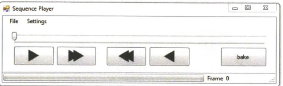
The sequence player can read and play the recorded assembly
sequence generated by the joint generator. It is a useful tool that
provides 4D assembly instructions for assembly or construction.
The disassembler is tool that generates disassembly sequence for
models that defined by planar surface contact constraints. This tool
can be used to evaluate the assembly sequence of complex geometric
assemblies other than interlocking frames.
1 Rhinoceros NURBS modeling for Windows, http://www.rhino3d.com/
2 Grasshopper- Generative Modeling for Rhino,
http://www.
5.1 Pattern Generator
The pattern generator uses a 2D pattern and a surface as input, and
produces a 3D interlocking pattern as output. Two different versions
of pattern generator are implemented: one applies a constant rotation
on every member; the other applies different degrees of rotation on
members based on their proximity to reference points or curves.
Both versions are implemented in the Grasshopper environment
using a customized python scripting component. The software also
provides a "intersection checker", which allows the user to input
the dimension for the members and identifies the problematic
intersection conditions in the assembly. The user is expected to fix
these conditions manually before proceeding to the Joint generator.
0
I~L
U
01
agd~-~
~tOHe
74
N:U- g -?5-- Q I C Q ao.*~ff
Fig. 5.1
Screenshots of Pattern Generator at
On: ka