Design and implementation of a secure energy-efficient hardware platform for wireless sensor networks

Design and Implementation of a

Secure Energy-Efficient Hardware Platform

for Wireless Sensor Networks

by

Madeleine Waller

B.S., Massachusetts Institute of Technology (2017)

Submitted to the Department of Electrical Engineering and Computer

Science

in partial fulfillment of the requirements for the degree of

Master of Engineering in Electrical Engineering and Computer Science

at the

MASSACHUSETTS INSTITUTE OF TECHNOLOGY

September 2018

c

○ Massachusetts Institute of Technology 2018. All rights reserved.

Author . . . .

Department of Electrical Engineering and Computer Science

August 21, 2018

Certified by . . . .

Anantha P. Chandrakasan

Vannevar Bush Professor of Electrical Engineering and Computer Science

Thesis Supervisor

Accepted by . . . .

Katrina LaCurts

Chair, Master of Engineering Thesis Committee

Design and Implementation of a

Secure Energy-Efficient Hardware Platform

for Wireless Sensor Networks

by

Madeleine Waller

Submitted to the Department of Electrical Engineering and Computer Science on August 21, 2018, in partial fulfillment of the

requirements for the degree of

Master of Engineering in Electrical Engineering and Computer Science

Abstract

Wireless sensor networks are networks of resource-constrained devices that collaborate to sense data about an environment and route it back to a resource-plenty gateway device that is connected to the Internet for processing. Oftentimes, wireless sensor networks are deployed in hazardous or hard to reach areas. For many sensor networks, securing these devices incurs an inhibitively high overhead cost, and tradeoffs must be made between security and energy efficiency, as the energy consumption of these nodes dictates their lifetime.

In previous work, a cryptographic accelerator [1] was proposed to speed up and reduce energy consumption of cryptographic primitives. The cryptographic accelerator is used in conjunction with a RISC-V processor to provide the flexibility to implement a wide range of security protocols. This work identifies common security threats in wireless sensor networks, and presents a hardware platform used to demonstrate the energy-efficient, cryptographic capabilities of the RISC-V security chip. We use the platform to test out various secure routing protocols on real hardware, and develop end-to-end energy models of our sensor node platform running these protocols. In developing these models, we seek to demonstrate that the RISC-V security chip can implement network security protocols at relatively little cost in a variety of different network configurations.

Thesis Supervisor: Anantha P. Chandrakasan

Acknowledgments

First, I would like to thank Prof. Anantha Chandrakasan for the opportunity to be a part of his research group, and for the guidance and support he has given me throughout the year. My time working with ananthagroup has been extremely rewarding, and I am incredibly grateful for the experience.

A huge thank you to my mentor Utsav, who has helped me scope and define my project throughout the year and tirelessly answered my many questions. Without his constant guidance, this project would not have been possible.

Lastly, thank you to my family and friends for your love and support. Dad - I love our odd engineering discussions that happen at all hours of the day, and I look forward to many more in the future.

Contents

1 Introduction 15

1.1 Motivation . . . 16

1.2 Wireless Sensor Networks . . . 16

1.2.1 WSN Topologies and Routing Protocols . . . 17

1.2.2 WSN Security Threats . . . 18

1.3 RISC-V Processor with Cryptographic Accelerator . . . 19

1.4 Thesis Contributions . . . 20

2 RISC-V Sensor Node Platform 21 2.1 Block Diagram and Components . . . 21

2.2 PCB Design . . . 23

2.2.1 PCB 4 Layer Compact Design . . . 23

2.2.2 PCB 2 Layer Demo Design . . . 23

3 Energy Profiling of BLE and RFM69HCW Radios 27 3.1 Bluetooth Low Energy (BLE) . . . 27

3.1.1 BLE RF Packet Structure . . . 28

3.1.2 SPI Communication with Radio Module . . . 31

3.1.3 BLE Energy Measurements . . . 32

3.2 RFM69HCW Packet Radio . . . 39

3.2.1 RFM69HCW RF Packet Structure . . . 40

3.2.2 SPI Communication with Radio Module . . . 41

4 eeDTLS over BLE Implemented on Sensor Node Platform 51 4.1 DTLS and eeDTLS Protocols . . . 51 4.2 Experimental Results: Sensor Node Communication Secured by eeDTLS 52 4.2.1 Relative Energy Consumption of System Components . . . 53 4.2.2 Sensor Node Lifetime . . . 57 4.2.3 Energy Analysis for Future Sensor Node with Custom Oscillator

and DC/DC Converters . . . 59

5 Securing Communication over RFM69HCW Transceiver in Mesh

Network Topology 63

5.1 Securing Mesh Networks: A Literature Survey . . . 64 5.1.1 IBC-Based Secure Routing Schemes in Flat Networks . . . 64 5.1.2 LEACH-Inspired Routing Schemes for Dynamic Clustered

Net-works . . . 65 5.2 HCBS Protocol over RFM69HCW on Sensor Node Platform . . . 67 5.2.1 Energy Trends: RF and Computation Energy of HCBS Protocol 70

6 Conclusion 79

6.1 Thesis Summary . . . 79 6.2 Future Work . . . 80

List of Figures

1-1 Classification of security threats to wireless sensor networks . . . 18

2-1 Sensor node block diagram . . . 22

2-2 PCB 4 layer CAD drawing with labeled components . . . 24

2-3 PCB 2 layer CAD drawing with labeled components . . . 25

2-4 Sensor node platform hardware setup with BLE radio peripheral . . . 25

3-1 BLE: star network topology . . . 28

3-2 BLE: mesh network topology . . . 29

3-3 Generic BLE 4.1 packet structure . . . 29

3-4 BLE 4.1 advertising packet structure . . . 29

3-5 BLE 4.1 data packet structure . . . 30

3-6 BLE advertising packets detected by RF sniffer . . . 30

3-7 BLE data packets detected by RF sniffer . . . 30

3-8 Current draw of BLE SPI Friend during BLE advertising event . . . . 33

3-9 Current draw of BLE SPI Friend during BLE connection event . . . . 33

3-10 Current draw of UART TX events of varying payload sizes . . . 35

3-11 Energy of UART TX events as a function of payload size . . . 36

3-12 BLE timing diagram to advertise, connect, and transmit data . . . . 38

3-13 RFM69HCW transceiver connected to our sensor node platform . . . 40

3-14 RFM69HCW generic variable-length packet structure . . . 41

3-15 Detailed RFM69HCW packet structure used in energy characterization 41 3-16 Current draw of RFM69HCW TX mode as function of output power level setting . . . 44

3-17 Payload width of RFM69HCW TX packets as a function of payload size with programmed bitrate 250 kbps . . . 45 3-18 RFM69HCW current measurements in primary operating modes, with

power level of TX mode set to 5 dBm . . . 47 3-19 Energy of RFM69HCW TX packets as a function of payload size for

power level 5dBm and bitrate 250 kbps . . . 48

4-1 Structure of DTLS-protected BLE 4.2 data packet . . . 52 4-2 Structure of eeDTLS-protected BLE 4.1 data packet . . . 52 4-3 Experimental Setup: sensor node connected to Internet via gateway

device and secured with eeDTLS . . . 53 4-4 Sensor node state diagram: eeDTLS Flow Chart . . . 54 4-5 Percent energy distribution of sensor node system components during

eeDTLS handshake . . . 55 4-6 Percent energy distribution of sensor node system components during

eeDTLS sensor data collection and transmission . . . 56 4-7 Percent power distribution of sensor node system components during

sleep state . . . 56 4-8 Breakdown of energy consumption of sensor node system components

during (a) eeDTLS handshake and (b) one sensor data collection and transmission for our current platform and a future platform with custom oscillator and buck converters . . . 60 4-9 Breakdown of power consumption of sensor node system components

during sleep state for our current platform and theoretical future plat-form with custom oscillator and buck converters . . . 61

5-1 Network diagram: sensor node connected to Internet via gateway device and running HCBS Protocol . . . 68 5-2 Sensor node state diagram: HCBS flow chart . . . 69 5-3 HCBS packet structure over RFM69HCW transceiver . . . 69

5-4 Modeled HCBS energy consumption as function of percent cluster heads and number of data collection events per round . . . 72 5-5 Modeled HCBS compute and RF energy . . . 72 5-6 HCBS energy plot: 2D cross sections . . . 73 5-7 Total energy as a function of percent cluster heads for (a) HCBS round

setup and (b) one data collection event . . . 75 5-8 3D plot for HCBS energy consumption without security overhead as a

function of percent cluster heads and number of data collection events for one round . . . 76 5-9 3D plot showing percent increase of HCBS energy caused by security

List of Tables

3.1 Breakdown of variables in BLE advertising mode energy equation . . 37 3.2 Breakdown of variables in BLE connection mode energy equation . . 38 3.3 Breakdown of variables in RFM69HCW TX packet energy equation . 46 3.4 Breakdown of variables in RFM69HCW Listen Mode duty cycle . . . 49

4.1 Breakdown of variables to calculate energy consumed by sensor node running eeDTLS in one year . . . 58 4.2 Total energy consumed by sensor node maintaining eeDTLS channel

for duration of 1 year with 1 time handshake and periodic data collec-tion/transmission . . . 58

5.1 Breakdown of RF and crypto computation events that occur in one round of the HCBS protocol . . . 71

Chapter 1

Introduction

With the advance of technology and the growing capability of microsensors, wireless sensing devices are becoming increasingly more prevalent in daily life. These inter-connected devices, commonly referred to as the Internet of Things (IoT), have the potential to positively impact our lives in a variety of ways, ranging from consumer convenience to hazard monitoring such as that of air/water quality or chemical hazards [2]. Wireless sensor networks make up an important subset of IoT and comprise of a network of nodes that make a collaborative effort to sense their environment and report the data back to some base station for processing. In this setup, sensor nodes are highly resource constrained, as they are battery powered devices intended to last for months or even years. Thus, providing security for wireless sensing devices is a challenging task; performing encryption and authentication adds computation and communication overhead, consuming precious energy in a resource constrained envi-ronment. This thesis introduces a sensor node platform that uses an energy efficient cryptographic hardware accelerator to minimize security overhead, and presents an end to end energy analysis of the encrypted sensor node operating under two different network schemes.

1.1

Motivation

Researchers believe the current number of interconnected IoT devices to be roughly 30 billion, estimating it to grow to over 75 billion by 2025 [3]. Although the number of interconnected devices is rising steeply, only a small fraction of these devices have adequate security – in 2015, roughly 90% of IoT devices collected personal data, and yet 70% of all IoT devices used unencrypted network services [4]. In February 2018, Trustwave released a survey highlighting the disparity between IoT adoption and the cybersecurity readiness of companies. The survey revealed that 64% of the surveyed organizations have deployed some level of IoT technology, and of those who have, 61% have had to deal with an IoT related security incident. Furthermore, only 10% of responders felt “very” confident that they could detect and protect against IoT-related security incidents [5].

The results of the aforementioned surveys demonstrate that while IoT networks and devices may be prevalent, the majority of organizations implementing these networks are not employing adequate security techniques. Clearly, there is a need for more ubiquitous security in IoT devices as a whole, yet implementing security for wireless sensor networks is a particularly daunting task, as a difficult tradeoff must be made between security and power resources [6].

1.2

Wireless Sensor Networks

Wireless sensor networks (WSNs) are networks of resource-constrained devices that collaborate to sense data about an environment and route it back to a resource-plenty gateway device, or “base station”, that is connected to the Internet for processing. WSNs are distinct from other wireless networks such as cellular or mobile ad-hoc networks due to several key characteristics. Firstly, they are highly decentralized and often operate in hazardous or hard to reach areas [2]. These sensor nodes are frequently deployed in an ad hoc manner and thus the network must be self-organizing. Simply acquiring the sensed data can be more important than knowing the IDs of

which nodes sent the data. Lastly, sensor nodes are highly resource constrained in terms of energy, memory, and processing capabilities. Due to the unique qualities of wireless sensor networks, myriad routing protocols have been tailored specifically to meet the needs of WSNs. Section 1.2.1 discusses typical network topologies of wireless sensor networks in addition to standard techniques used for routing data collected back to a gateway device.

1.2.1

WSN Topologies and Routing Protocols

Wireless sensor networks can be broadly classified by the following aspects: network topology and protocol operation. A very basic network topology is the star network topology, in which sensor nodes only communicate with some gateway device. In many WSNs, not all nodes can easily communicate with the gateway device, resulting in a mesh network - a network in which nodes route data through each other to reach the gateway device. Mesh network topologies fall into two main categories: flat networks and hierarchical networks. In flat networks, all nodes are considered to be peers and a routing protocol selects some sequence of nodes to form a path back to the gateway device. Hierarchical networks divide the network into clusters, in which cluster heads aggregate and reduce data from cluster members to save energy and, in some protocols, also relay data from other cluster heads to the gateway device [7].

Routing protocols describe the algorithm used to route sensor data back to the gateway device, and can be categorized by their common high level characteristics, e.g. data-centricity, location-based routing, multipath-based, query-based routing and quality of service [2, 8]. Data-centric algorithms focus on aggregating and transmitting data efficiently, without focusing on the ID of the sensor node that detected the data. Location-based algorithms use position information to relay data to desired regions rather than the entire network. Multipaths are used when fault tolerance and reliability is critical. Query-based algorithms only transmit sensed data when the gateway device first expresses interest in receiving the data. Quality of service focused algorithms ensure that quality requirements such as delay, energy, or bandwidth are met when delivering data to the gateway device.

1.2.2

WSN Security Threats

In the context of security, there are several key themes that all protocols seek to achieve: confidentiality, integrity, and authentication in addition to availability, access control, and nonrepudiation [2]. Securing WSNs is a uniquely difficult challenge, as WSNs are vulnerable to standard attacks that can occur between traditional devices, in addition to a whole host of new attacks that take advantage of the resource constrained and dynamic nature of WSNs.

Security protocols proposed in academic literature assume threat models against adversaries with varying degrees of capabilities. Adversaries can be divided into three main types depending on their capabilities: passive, active, and compromising. A passive adversary simply eavesdrops on communications, thereby threatening privacy of communication. Active adversaries can tamper with the data and threaten control and availability of the network. A compromising adversary is the most powerful, as it can compromise and access secret keys of trusted network nodes [9].

Figure 1-1: Classification of security threats to wireless sensor networks, taken from [2]

Figure 1-1 presents a diagram of some common attacks in wireless networks, which can be divided into three main categories: threats to privacy, threats to control, and threats to availability [2]. Threats to privacy are passive attacks in which the attacker simply listens in on the network. Threats to control involve radio interference and environmental tampering, or more targeted attacks to network packets. Selective forwarding attacks consist of hijacking a sensor node and only forwarding a specific subset of data as desired by the adversary. Sybil attacks are impersonation attacks in which a malicious node collects several identities in the network, either by generating new identities or by stealing the identity of legitimate nodes and can affect applications such as data aggregation. In Byzantine attacks, an external adversary compromises multiple authenticated nodes and attacks the network from within. Threats to availability occur when an attacker floods the network with packets, jams a frequency band with a high power transmitter, or deliberately triggers collisions that result in nodes exhausting their resources trying to retransmit packets. Laptop class adversaries are a unique threat to WSNs, as they are considered resource-rich adversaries that can attack and exhaust the physical resources of sensor nodes without straining their own resources.

1.3

RISC-V Processor with Cryptographic

Accelera-tor

Securing wireless sensor networks comes at the cost of added RF energy and a prohibitively high computation cost in software-only implementations. To reduce the overhead of cryptographic computation, researchers in [1] developed dedicated hardware accelerators for cryptographic functions, which work in conjunction with a RISC-V processor to support network security protocols. The chip was designed specifically to improve energy efficiency of the Datagram Transport Layer Security (DTLS) protocol, and accomplishes a 438x energy savings over an equivalent software only implementation. The RISC-V security chip is reconfigurable and allows a user to

re-purpose the chip’s elliptic curve cryptography primitives for other security schemes. For instance, the chip is capable of a 230x energy savings for running ECMQV, an alternative to ECDHE+ECDSA-based authenticated key exchange. In this work, we exploit the capabilities of the RISC-V security chip to secure a custom sensor node platform in several network configurations.

1.4

Thesis Contributions

The objectives of this research are to design a sensor node platform to demonstrate the energy-efficient, cryptographic capabilities of the RISC-V Security Chip, and to perform a complete energy characterization of the sensor node platform when running different security and routing protocols.

Chapter 2 provides an overview of the sensor node platform and some of the design decisions that went into building it. Chapter 3 presents an energy model developed to characterize two different types of radios that our platform supports: a BLE 4.1 transceiver for master/slave communication in star networks and an RFM69HCW packet transceiver for multipoint communication in mesh networks. Chapter 4 provides a brief overview of the eeDTLS protocol, an efficient version of the Datagram Transport Layer Security protocol proposed in [10], and presents an end-to-end energy characterization for running this protocol to protect sensor data collected on our sensor node platform. Chapter 5 presents a literature survey of techniques used to secure mesh networks, and presents an energy characterization study of the cost to run a Hybrid Cryptography-Based Scheme on our platform, in addition to an analysis of the security overhead of the protocol. Chapter 6 summarizes the key contributions of this thesis and proposes potential directions for future work.

Chapter 2

RISC-V Sensor Node Platform

2.1

Block Diagram and Components

Wireless sensor nodes consist of one or more sensing devices, a transceiver, and a microcontroller to handle state and control communication via RF. As such, to demo the RISC-V security chip described in Section 1.3, the sensor node platform design includes a custom printed circuit board (PCB) with the following main components:

∙ Battery protection circuitry to allow for battery or microUSB power supply

∙ Custom chip with RISC-V processor and cryptographic hardware accelerator [1]

∙ 2 sensors: LIS3DE accelerometer and LM95071 temperature sensor

∙ SPI breakout header for connection to variety of radios

∙ MicroSD socket, with SD card for program storage

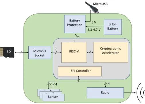
Figure 2-1 presents a high level block diagram of our sensor node platform. For battery charging protection, we selected an LTC4063 chip, a Linear Technologies Li-Ion charger with a low dropout linear regulator that provides smart recharge, under voltage lockout protection, and LDO current limiting. We have configured the LTC4063 to output 3.3 𝑉 , powered by a rechargeable Lithium Ion 3.7V battery and/or via 5 𝑉 microUSB. We use additional linear dropout regulators to supply 2.5 𝑉 and

Figure 2-1: Sensor node block diagram

1.2 𝑉 to power the RISC-V chip. To monitor the power consumption on our board, we’ve included series resistors to measure current at the output of our LTC4063 chip supplying 3.3 V, and at the output of the LDOs supplying 2.5 V and 1.2 V.

The processor interfaces with the two sensing devices and desired radio via SPI. Breakout headers connect to the processor’s hardware SPI pins - clock, master in slave out (MISO), and master out slave in (MOSI) - and 10 unused GPIO pins, to simplify adding future functionality to the existing platform, e.g. interfacing with additional sensing devices. When reading sensor data over SPI, we read 1 byte of temperature data from the LM95071 chip, and 4 bytes of data from the LIS3DE chip: 1 byte temperature data, and 1 byte accelerometer data per each axis X, Y, and Z.

The sensor node platform currently has coding infrastructure in place to interface with two radios: Adafruit’s BLE SPI Friend [11] and Sparkfun’s RFM69HCW Packet Radio [12]. We selected these radios to test and demo the sensor node under two different network schemes, a BLE master/slave topology in which all sensor nodes are slave devices that communicate directly with a master gateway device via DTLS, and a mesh network topology in which sensor nodes encrypt and route data through each other to reach a gateway device. These radios are discussed further in Chapter 3.

The PCB connects a microSD socket to the RISC-V chip via Secure Digital Input Output (SDIO) protocol. The microSD holds program data, providing non-volatile memory storage that can be used to boot the processor on power up. The SD card is not used in the final sensor node demo because we had difficulties in setting up the SD socket on the PCB in SDIO mode, due to signal integrity issues. As a workaround, an Opal Kelly XEM7001 FPGA board was used to emulate the SD card. Section 2.2 includes a compact 4-layer board design with SD card and a to 2-layer board design that acted as the final platform demo, interfacing with the FPGA workaround.

2.2

PCB Design

2.2.1

PCB 4 Layer Compact Design

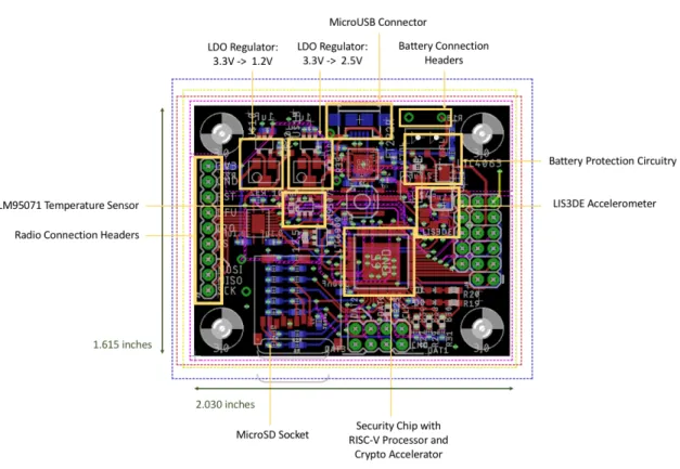
The 4 layer PCB design shown in Figure 2-2 is an Eagle CAD drawing of a compact board design with dimensions 1.615 in x 2.030 in. The copper pour in the top, second, and bottom layers (shown in red, yellow, and blue respectively) are connected to ground, and the third layer (shown in pink) is a VDD layer split into two sections -the copper pour in -the top section is connected to 3.3 V and -the bottom is connected to 2.5V.

The battery protection circuitry is located in the upper portion of the PCB where the VDD layer is 3.3V, and the RISC-V security chip and all its peripherals are located in the lower portion of the PCB, see Figure 2-2 component labels for details. Note that the copper pours are shown as dotted lines external to the board rather than filled in to allow visibility of components. As Figure 2-2 demonstrates, routing occurs primarily in the top and bottom layers; the Vdd layer contains remaining routing that did not fit in the outer layers, leaving layer 2 as a ground plane.

2.2.2

PCB 2 Layer Demo Design

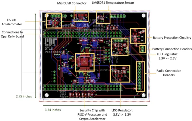
The 2 layer PCB design shown in Figure 2-3 has dimensions 2.75 in x 3.34 and consists of a top layer (red) and bottom layer (blue). The copper pour in both layers is

Figure 2-2: PCB 4 layer CAD drawing with labeled components

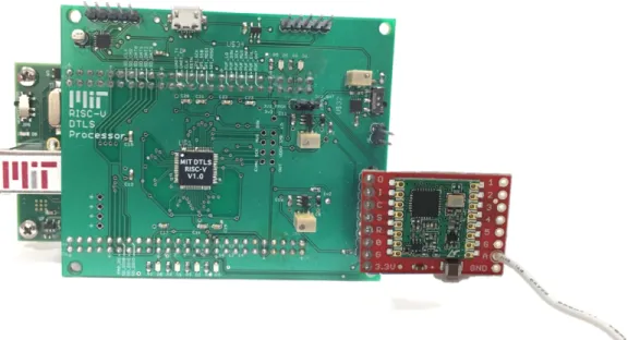
connected to ground. The white outline extending past the left boundary of the board marks the edge of the Opal Kelly FPGA board used simulate the SD card. The fabricated and assembled board is shown in Figure 2-4, connected to a BLE radio and Opal Kelly board.

Figure 2-3: PCB 2 layer CAD drawing with labeled components

Chapter 3

Energy Profiling of BLE and

RFM69HCW Radios

This chapter presents an overview of the BLE and RFM69HCW transceivers used in our sensor node platform, how to interface with them, and a complete energy characterization of the two transceivers, to be used in end to end energy analyses in later sections.

3.1

Bluetooth Low Energy (BLE)

Bluetooth Low Energy (BLE), a key feature of the Bluetooth v4.0 Core Specification [13], is a popular protocol used for radio communication in IoT devices due to its simple protocol stack, low power consumption, robust radio, and compatibility among a wide variety of manufacturers [14]. We chose BLE over other short-range transceivers such as Zigbee because BLE consumes less energy and has a very attractive ratio of energy per bit transmitted [15].

Our BLE radio module, an Adafruit chip with an nRF51822 BLE SoC, has a limited range of 10 meters between transceivers [11] and supports the following network setup: a low power sensor node (slave device) wakes up to send data directly to a gateway device (master device) before returning to sleep mode to conserve energy. This setup lends itself to a star network topology in which multiple sensor devices

interact with a single gateway device, as shown in Figure 3-1.

Figure 3-1: BLE: star network topology

In 2017, Bluetooth released a Bluetooth Mesh Specification as part of BLE 5.0, introducing support for a "managed-flood-based" mesh network [16]. Figure 3-2, pulled from the Bluetooth Mesh Specification v1.0, presents a sample BLE mesh network topology. The managed-flood-based network proposed is not a true peer to peer mesh network topology. Rather, it is a hierarchical topology that relies on dedicated relay nodes and a new concept called "friend nodes." To send sensor data, sensor nodes send data packets to relay nodes, and relay nodes broadcast the packets until they reach a gateway device, thereby extending the range of the original sensor nodes. Friend nodes connect low power nodes to the network – since low power nodes wake up only periodically to save power, friend nodes receive packets for the low power nodes in their absence, and relay the packets accordingly to mitigate dropped packets that would otherwise occur when the low power node was asleep.

We do not test BLE in a mesh network configuration, as our current BLE hardware only supports up to BLE 4.1 and BLE mesh is introduced in BLE 5.0. Thus, we focus on characterizing the energy profile of a BLE radio operating in slave mode in a master-slave topology, which we use to develop an end-to-end characterization of the energy profile of our sensor node running an energy efficient version of DTLS over BLE, discussed in detail in Chapter 4.

3.1.1

BLE RF Packet Structure

The BLE RF Packet Structure is dictated by the BLE protocol stack. According to the BLE 4.1 core specification, BLE’s physical layer is an RF channel operating at

Figure 3-2: BLE: mesh network topology [16]

2.4GHz. Built atop the physical layer, a link layer consists of data packets with the following fields: preamble byte, access address, payload data unit (PDU), and cyclic redundancy check (CRC) [17], as shown in Figure 3-3. There are two types of PDU channels at the link layer: an advertising channel PDU and a data channel PDU.

Figure 3-3: Generic BLE 4.1 packet structure

When a sensor node is ready to send data, it powers the BLE radio module and sends advertising packets, waiting for a BLE master device to accept and initiate a connection. Figure 3-4 shows the structure of the BLE advertising packets: within the link layer payload field, there is a 2 byte advertising PDU header, followed by 6-37 bytes of advertising data.

Figure 3-4: BLE 4.1 advertising packet structure

data packets consist of a 17 byte overhead, and a 0-20 byte data payload. The 17 bytes of overhead occur at several different layers in the BLE protocol stack. 8 bytes occur at the link layer, shown in gray in Figure 3-5. 2 bytes are due to the PDU Data channel header. The Logical Link Control and Adaptation Protocol (L2CAP) Layer adds a 4 byte header, used to provide data encapsulation services to the upper layers. The Attribute (ATT) layer and Generic Attribute Profile (GATT) layers add an additional 3 byte overhead to provide a service framework that support data communications between any two devices connected over BLE [17],[18],[19],[20].

Figure 3-5: BLE 4.1 data packet structure

To verify these packet structures, we used a Texas Instruments SmartRF Packet Sniffer to measure the advertising and data packets of the BLE radio module we used, a "BLE SPI Friend" developed by Adafruit that includes an nrF51822 system on chip (SoC) running the BLE 4.1 protocol stack. Figure 3-6 and Figure 3-7 show screenshots of the RF Sniffer results, detecting advertising packets and data packets sent by our BLE radio module respectively.

Figure 3-6: BLE advertising packets detected by RF sniffer

3.1.2

SPI Communication with Radio Module

We chose Adafruit’s BLE SPI Friend for the BLE radio module in our setup due to its simple SPI interface. The radio module has an nRF51822 RF SoC with an ARM Cortex M0 32-bit processor that implements SDEP, a binary protocol developed by Adafruit for SPI communication. We use SDEP for two primary types of communications: setting characteristics pertaining to BLE advertising and connection, and sending sensor data to the radio module for wireless transmission.

When enabled, the radio module sends out advertising RF packets at periodic intervals until a master device receives the packets and initiates a connection. Once connected, RF "connection events", consisting of back and forth transmission between the BLE peripheral and master device, occur periodically to maintain the established connection until the connection is closed [15]. The rate of both the advertising and connection intervals affect the energy consumption of the radio and thereby the sensor node’s lifetime; these rates can be set by the sensor node to optimize for a target application. Over SDEP, we can set the interval between advertising events directly, but since the master device controls the connection events, we set a minimum and maximum interval during which the master device can initiate the connection event.

To send sensor data for radio transmission, we must fragment our data into 16 byte payloads. The radio module has a 20 byte buffer on chip, allowing for asynchronous transmit and receive. However, due to this buffer size, SDEP messages are ≤ 20 bytes and have the following data structure: a 4 byte header, followed by a 0-16 byte payload. Note that this imposes an extra limitation on our maximum data payload: while BLE 4.1 supports up to a 20 byte data payload, the buffer size limits communication to a 16 byte data payload due to the 4 byte SDEP overhead, even though the SDEP overhead is not transmitted over the air [21].

3.1.3

BLE Energy Measurements

To characterize the energy profile of our radio module, we performed measurements of the instantaneous current consumption as a function of time under the following operating scenarios: standby mode to calculate processor overhead, advertising mode to characterize advertising packets, and connection mode to characterize connection events and data transmission. To gather current data, we added a 9.9 ohm series resistor to the 3.3V power supply, and used an oscilloscope to measure voltage across the resistor, amplified by a differential amplifier for ease of measurement. We calibrated the differential amplifier and found the following linear relationship between the amplified voltage measured and the actual voltage across the resistor, such that G is gain and 𝑉𝑂𝐹 𝐹 is the DC offset of the amplifier:

𝑉𝑀 𝐸𝐴𝑆[𝑉 𝑜𝑙𝑡𝑠] = 𝐺 × 𝑉𝑅𝐸𝑆 + 𝑉𝑂𝐹 𝐹 = 21.3 × 𝑉𝑅𝐸𝑆 + 0.235

Using this signal, we know the current drawn by the radio module at any given timestep: 𝐼[𝐴𝑚𝑝𝑠] = 𝑉𝑅𝐸𝑆 𝑅 = (𝑉𝑀 𝐸𝐴𝑆− 0.235)/21.3 9.9 .

All of our measurements in the following section were taken at a sampling rate of 250 kHz, and smoothed with a small window averaging filter of 20 samples to mitigate measurement noise.

Results and Energy Model

This section presents an energy model for the BLE SPI Friend radio. As explained in Section 3.1.1, BLE packets fall into two primary categories: advertising packets and data packets; correspondingly, the BLE transceiver operates in two primary states: advertising mode in which the transceiver is broadcasting advertising packets, and connection mode in which the sensor node is maintaining a channel with a master

device and sending sensor data bytes.

Figure 3-8: Current draw of BLE SPI Friend during BLE advertising event

Figure 3-9: Current draw of BLE SPI Friend during BLE connection event

Figure 3-8 shows the current drawn by the BLE SPI Friend to transmit a single advertising packet, and Figure 3-9 shows the current drawn to perform a connection event. According to the nRF51822 datasheet, BLE transmit current varies from 4.7

mA to 11 mA when powered at 3V, depending on the output power level [22]. We do not set the output power level directly, simply noting that our advertising event falls withing this acceptable current range. Unlike advertising events, a connection event consists of both transmitting and receiving bytes to maintain the channel with the master device. According to specification, the RX current draw of the nRF51822 is 9.7 mA. We did not study the timing of the connection event in detail, but we do note that our connection event current draw falls within the acceptable range for both transmit and receive.

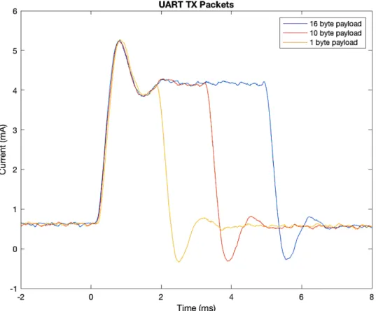
Through our measurements of the BLE transceiver, we’ve identified a third source of high current draw that we’ve titled "UART TX events", in which our BLE module draws high current when sensor data is transmitted over BLE using a UART service, a proprietary GATT service specified by Nordic Semiconductors that simulates a basic UART connection [23]. Figure 3-10 shows a plot of instantaneous current vs. time for data packets with payloads of 1 byte, 10 bytes, and 16 bytes.

To calculate the energy of advertising events, connection events, and UART TX events, we used Matlab to detect the start and endpoints (shown as red and yellow dots in Figures 3-8 and 3-9), and performed the following conversion from current to energy:

𝐸𝑒𝑣𝑒𝑛𝑡=

∫︁ 𝑡𝑒𝑛𝑑

𝑡𝑠𝑡𝑎𝑟𝑡

𝑉𝐷𝐷× 𝐼(𝑡)𝑑𝑡

such that 𝑡𝑠𝑡𝑎𝑟𝑡 and 𝑡𝑒𝑛𝑑 are the start and endpoints of a high current event, 𝑉𝐷𝐷

is the 3.3 V power supply, and 𝐼(𝑡) is current as a function of time. We found the typical energy of a single advertising event 𝐸𝐴𝐸 to be 74.472𝜇𝐽 , excluding energy

due to processor overhead of the radio module. Note that this measurement is the same order of magnitude as that measured in [15], in which they measure the energy of advertising packets of a CC2540 transceiver to consume 100𝜇𝐽 when powered at 3𝑉 . For our connection events, we found a linear relationship between energy (Joules) of the connection event 𝐸𝐶𝐸 and the time interval 𝑇𝐼𝑁 𝑇 𝐶 (in seconds) between

consecutive connection events:

Figure 3-10: Current draw of UART TX events of varying payload sizes

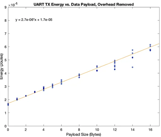
We also measured a linear relationship between the energy of UART TX events and payload size, 0-16 bytes, as seen in Figure 3-11. This energy relationship can be extrapolated to calculate the UART TX energy of any number of payload bytes 𝑛 by the following linear step equation, assuming 𝑛 > 0:

𝐸𝑇 𝑋(𝑛) = 𝑛 × 2.7 × 10−6+ ⌈︃ 𝑛 16 ⌉︃ ×1.7 × 10−5

In the above energy calculations, we exclude the contribution of processor overhead, as we account for it separately in our energy model. Processor overhead pulls a constant current draw of 0.28291 mA when the radio is powered, which we account for by calculating its average power to be 𝑃𝑃 𝑅 = 𝐼 × 𝑉𝐷𝐷 = 0.28291 × 3.3 = 0.93𝑚𝑊 . Thus,

Figure 3-11: Energy of UART TX events as a function of payload size

the energy of processor overhead can be written as a function of time:

𝐸𝑃 𝑅(𝑡) = 𝑃𝑃 𝑅 × 𝑡 = 9.3 × 10−4× 𝑡

Note that our raw current measurements also include the constant current offset drawn by a blue LED whenever the radio is in connection mode for ease of testing. The LED overhead is ignored in our energy calculations of UART TX and connection events, as it is a convenience for testing that would not be deployed in a final sensor node.

Using the aforementioned calculations, we present an energy model that includes the total energy for our sensor node to wake up and send sensor data. The energy model is split into two primary equations: the energy of the broadcast window in which the node is advertising 𝐸𝐴𝐷𝑉, and the energy of the connection window in

Table 3.1 explains the variables that contribute to the total advertising energy. The energy of advertising is dictated by the number of advertising events that occur and the energy due to processor overhead:

𝐸𝐴𝐷𝑉 = ⌈︃ 𝑇𝐴𝐷𝑉 𝑇𝐼𝑁 𝑇 1 + 1 ⌉︃ × 𝐸𝐴𝐸+ 𝑃𝑃 𝑅× 𝑇𝐴𝐷𝑉

Table 3.1: Breakdown of variables in BLE advertising mode energy equation

𝑇𝐼𝑁 𝑇 1 time between advertising packets in the range

0.02 ≤ 𝑇𝐼𝑁 𝑇 1 ≤ 10.24 seconds

𝑇𝐴𝐷𝑉 time spent in advertising mode

𝐸𝐴𝐸 energy of one advertising packet: 74.472𝜇𝐽

𝑃𝑃 𝑅 average instantaneous power of processing overhead, 0.93mW

The total connection energy is calculated similarly. We approximate that for every UART TX packet, there is one connection event, and we estimate the total time spent in connection mode 𝑇𝐶𝑂𝑁 𝑁 as a function of the number of connection intervals

that occur before disconnection. Table 3.2 lists the relevant variables in the following equation for total energy in connection mode 𝐸𝐶𝑂𝑁 𝑁:

𝐸𝐶𝑂𝑁 𝑁 = ⌈︃ 𝑛 16 ⌉︃ × [︃ 𝐸𝐶𝐸(𝑇𝐼𝑁 𝑇 2) + 𝑃𝑃 𝑅× 𝑇𝐼𝑁 𝑇 2 ]︃ + 𝐸𝑇 𝑋(𝑛)

To get the total energy cost of transmitting data bytes over BLE, we simply add the energy cost of advertising and connection together. Figure 3-12 presents a timing diagram of the key elements of the advertising and connection phases that we’ve discussed in our energy calculations. The timing diagram highlights the periodicity of advertising events and connection events, 𝑇𝐼𝑁 𝑇 1 and 𝑇𝐼𝑁 𝑇 2 respectively as referenced

in previous equations, and identifies the three primary high current events that we’ve studied in this section and identified as the main source of energy consumption during sensor data transmission.

Table 3.2: Breakdown of variables in BLE connection mode energy equation

𝑛 number of sensor data bytes sent, 𝑛 > 0

𝐸𝐶𝐸(𝑇𝐼𝑁 𝑇 2) energy of one connection event, as a function of connection

interval 𝑇𝐼𝑁 𝑇 2

𝑇𝐼𝑁 𝑇 2 upper limit of the connection interval range, such that

0.01 < 𝑇𝐼𝑁 𝑇 2 < 4 seconds

𝑃𝑃 𝑅 average instantaneous power of processing overhead, measured

to be 0.93 mW

𝐸𝑇 𝑋(𝑛) energy of UART TX as function of n bytes

Figure 3-12: BLE timing diagram to advertise, connect, and transmit data

The BLE radio module receives UART RX packets using the same UART GATT service used to transmit. The receipt of these packets occur as part of the connection events, causing the connection events to be a little bit wider rather than occurring as a separate high current event. We attempted to measure the energy for BLE to

receive packets, but had difficulties with identifying when the transceiver received the UART data packets vs. generic channel back and forth communication. As a rough approximation to generate our energy models in Chapter 4, we assume that because the current to receive is approximately twice that to transmit over BLE, the energy 𝐸𝑅𝑋 of the BLE transceiver is twice the energy of an equivalent 𝐸𝑇 𝑋. This is a rough

estimation that, in future work, requires further study to generate a more accurate model.

3.2

RFM69HCW Packet Radio

The RFM69HCW packet radio is an RF module capable of operating over a wide programmable range of frequencies, including the 315 MHz, 433 MHz, 868 MHz and 915MHz Industry Scientific and Medical (ISM) RF bands. The transceiver supports frequency shift keying, minimum shift keying, and on/off keying modulations [24]. Additionally, it supports a symmetric link for communication between devices and can thus be paired with any many-to-many network communication scheme, allowing us to try out different mesh network routing schemes and test a variety of capabilities of the RISC-V security chip.

Our current setup includes a RFM69HCW module distributed by Sparkfun, op-erating at 915 MHz, an unlicensed band frequently used for local area networks in North America [25]. Figure 3-13 shows the RFM69HCW connected to our sensor node platform. The range of the RFM69HCW transceiver is much higher than that of the aforementioned BLE transceiver module - the BLE transceiver can only support links up to 10 meters, whereas with a basic wire antenna, the RFM69HCW transceiver supports a link for up to several hundred meters outside, with no obstructions. Indoors it can operate up to around 50 meters, despite obstructions such as multiple walls [12]. This higher range comes at the cost of higher current draw. Note that the range of the radio is affected by the data rate selected and the power level chosen; thus a tradeoff must be considered when optimizing for range and battery life.

Figure 3-13: RFM69HCW transceiver connected to our sensor node platform

3.2.1

RFM69HCW RF Packet Structure

The structure of RFM69HCW RF packets is very simple and flexible. All packets sent via the RFM69HCW transceiver consist of the following fields: preamble, sync word, payload, and optional CRC bytes. Unlike BLE, there are no advertising and connection phases between two devices; when a node wishes to contact a device, it broadcasts its data packet and can optionally include an address byte so that all nodes except the desired receiving node ignore the packet.

According to its datasheet, the RFM69HCW transceiver that we have chosen operates at 915 MHz and can send three different packet types: packets with a theoretical unlimited length payload in which there is no length or CRC field, packets with fixed length payload that have CRC but no length field (communicating devices agree on payload length separately), and packets with variable length payload and CRC [24], which we focus on in this paper. Figure 3-14 shows a generic packet structure used by the RFM69HCW to deliver a variable length payload. The theoretical maximum payload for a variable length packet with CRC is 255 bytes, but to use the on chip FIFO of the RFM69HCW allowing for simple communication between our processor and the transceiver over SPI, we are limited to a 66 byte payload as shown in Figure

3-15.

Figure 3-14: RFM69HCW generic variable-length packet structure

Figure 3-15: Detailed RFM69HCW packet structure used in energy characterization

Note that the payload field is further reduced to a range of 0-61 bytes of sensor data, due to five overhead bytes stored in the 66-byte FIFO: a recipient address byte, sender address byte, and a control byte enabling a simple network structure, and two CRC bytes. The CTL byte indicates a request for an acknowledgement packet affirming the receipt of the data packet; when an acknowledgement is requested, the receiving node responds with a regular variable-length packet, including an acknowledgement CTL byte and a zero byte data payload to confirm that it received the data packet from the sender.

3.2.2

SPI Communication with Radio Module

The RFM69HCW module supports SPI communication via a low-level protocol in which a microcontroller reads and writes directly to registers on board the radio module to set system parameters, send RF packets, and check for receipt of RF packets. To read/write to a register, the microcontroller asserts chip select, sends a 1 byte register address, reads from or writes to the specified register, then de-asserts chip select. The RFM69HCW datasheet provides a complete list of registers onboard the device [24]. To aide communication with the RFM69HCW transceiver, we designed our own C library to interface between the RISC-V and the radio module, drawing from an

Arduino C++ library developed by LowPowerLab and an incomplete C library found on Github [26],[27]. The library initializes the radio at startup and interfaces with the radio in real time to perform RF send and receive operations. A useful feature of the RFM69HCW is a programmable bitrate between 1.2-300 kbps, and a programmable power level that allows for transmission output from 5 dBm to 20 dBm.

When powered, the RFM69HCW transceiver operates in five modes: sleep, synthe-sizer, standby, receive, and transmit. Sleep mode is the radio’s lowest power mode, drawing only 0.1𝜇𝐴 according the the RFM69HCW datasheet [24]. Standby mode is the transceiver’s idle mode, which the radio must pass through before entering both the transmit and receive modes. In low power applications, a "listen mode" can be layered on top of standby mode, allowing the radio to have a duty cycle in which it enters receive mode periodically, and spends the rest of the time in a lower power idle mode, drawing 1.2𝜇𝐴.

Synthesizer mode occurs at wake up from sleep mode or power on, to set up a frequency synthesizer and allow the phase-locked loop (PLL) of the transceiver to lock. In receive mode, the receiver is powered on; when it detects a packet, it stores the packet in the on chip FIFO and raises an interrupt, signalling the microcontroller to read from the FIFO and clear the interrupt. In transmit mode, the radio actively transmits at all times. If the FIFO is not yet ready to be read, it transmits preamble bits "010101" repeatedly; when the FIFO is ready, the transceiver transmits the packet stored in the FIFO over RF and raises an interrupt when done, indicating to the microcontroller to switch to a different, lower power mode. Note that the transceiver cannot switch modes on its own; the library selects when to switch modes at all times, and polls the interrupt pin frequently to enable quick transitions out of the high power transmit and receive modes.

3.2.3

RFM69HCW Energy Measurements

To characterize the energy profile of the RFM69HCW radio module, we performed measurements of the instantaneous current consumption as a function of time. We measured the current directly by supplying the radio via a Keithley 2400 Source meter. Note that we attempted this setup to measure BLE current consumption as well, but BLE packets have smaller packet widths and thus we could not sample at a fast enough rate to adequately capture their shape.

Results

This section presents an energy model for sending sensor data with the RFM69HCW radio. As explained in Section 3.2.2, the RFM69HCW radio operates in five primary modes: sleep, standby, synthesizer, receive, and transmit. We did not measure current draw in synthesizer or standby mode, as the time spent in both of these modes is negligible. We used the datasheet’s approximation of 0.1𝜇𝐴 for sleep mode current draw, as we found the sleep mode current to be indistinguishable from our measurement noise. Since we use the RFM69HCW to build a mesh network, sensor nodes may spend significant time receiving and re-broadcasting in order to route messages sent by other nodes. Thus, our energy model to send sensor data includes the energy to transmit bytes, receive bytes, and energy to wake up and listen in receive mode as a function of duty cycle and time.

There is no current associated with receiving a packet; rather, it is simply the current drawn when the RF transceiver is in receive mode, regardless of how many packets are received and at what bitrate. We measured the typical current in receive mode to be 15.3𝑚𝐴, slightly less than the 16𝑚𝐴 stated in the datasheet. Current draw associated with RF transmission is more complicated, as the RFM69HCW allows for programmable bitrate and output power level settings. We found the magnitude of current draw to be a function of output power level. The output power level allows for setting an arbitrary programmable range from 0-31, which according to

the datasheet, correlates linearly over the output power range 5 dBm to 20 dBm. Figure 3-16 shows the relationship we found between magnitude of current draw and discrete output power level. Note that in taking these current measurements and all

Figure 3-16: Current draw of RFM69HCW TX mode as function of output power level setting

other measurements in this section, we supplied the transceiver with 𝑉𝐷𝐷 = 2.5𝑉 to

minimize power consumption, as this was the minimum voltage level at which the radio received packets consistently.

To study the relationship of TX mode current and bitrate, we took current measurements of TX mode at bitrates ranging from 1.2 kbps to 300 kbps. We found no correlation, therefore, we picked the highest bitrate possible to minimize time in the high power TX mode and consequently minimize transmission energy. We selected 250 kbps, as above this bitrate we had difficulties receiving packets despite the radio’s theoretical maximum bitrate of 300 kbps. Note that in applications where high range

is important, a lower bitrate may be optimal, as a higher bitrate typically reduces RF range.

We studied the relationship between transmission packet width and payload size at 250 kbps to verify the accuracy of the programmable bitrate and measure transmission overhead. Figure 3-17 shows the slope of packet widths vs payload size is 3.2 × 10−5 𝑠𝑒𝑐𝑜𝑛𝑑𝑠/𝑏𝑦𝑡𝑒𝑠. To convert to bits per second, we calculated:

Figure 3-17: Payload width of RFM69HCW TX packets as a function of payload size with programmed bitrate 250 kbps

1

3.2 × 10−5 _{𝑠𝑒𝑐/𝑏𝑦𝑡𝑒𝑠} × 8 𝑏𝑖𝑡𝑠/𝑏𝑦𝑡𝑒𝑠 = 250.0 𝑘𝑏𝑝𝑠

, which matches the programmed bitrate perfectly. Note the nonzero offset at payload size zero in Figure 3-17; in our measurements, we found this offset to be 0.55 𝑚𝑠 for 250𝑘𝑏𝑝𝑠, though this number varies as a function of bitrate. Thus, we have the following relationship between the width in seconds of a single transmission packet

𝑇𝑇 𝑋_𝑃 𝐴𝐶𝐾𝐸𝑇 and an 𝑛 byte payload, such that 0 ≤ 𝑛 ≤ 61:

𝑇𝑇 𝑋_𝑃 𝐴𝐶𝐾𝐸𝑇(𝑛) =

8

250 × 106 × 𝑛 + 5.5 × 10 −4

To build an energy model, we developed equations for three separate events in which the radio consumes power: packet transmission, packet receive, and energy of duty cycle to wake up and power on receive to check for packets. To calculate data transmission energy from our current measurements, we perform the same integral introduced in Section 3.1.3:

𝐸𝑝𝑎𝑐𝑘𝑒𝑡 =

∫︁ 𝑡𝑒𝑛𝑑

𝑡𝑠𝑡𝑎𝑟𝑡

𝑉𝐷𝐷× 𝐼(𝑡)𝑑𝑡

Unlike the abnormal shape of BLE high current events, the shape of the current profiles for TX/RX as a function of time are simple step functions that can be approximated by the area of the rectangle - Figure 3-18 shows the radio alternating between sleep and receive mode, with a thin peak near 6000 ms in which the transceiver enters TX mode to transmit a data packet.

We can calculate the energy of a single TX packet with the following equation:

𝐸𝑇 𝑋_𝑃 𝐴𝐶𝐾𝐸𝑇(𝑛) = 𝑉𝐷𝐷× 𝐼𝑇 𝑋× 𝑇𝑇 𝑋_𝑃 𝐴𝐶𝐾𝐸𝑇(𝑛)

Table 3.3 includes a breakdown of the variables used to characterize 𝐸𝑇 𝑋_𝑃 𝐴𝐶𝐾𝐸𝑇.

Table 3.3: Breakdown of variables in RFM69HCW TX packet energy equation

𝑉𝐷𝐷 voltage supply, 2.5 𝑉

𝐼𝑇 𝑋 current as a function of output power level, see Figure 3-16

𝑛 number of sensor data bytes sent in payload, 0 ≤ 𝑛 ≤ 61 𝑇𝑇 𝑋_𝑃 𝐴𝐶𝐾𝐸𝑇 width of packet as function of bitrate and payload size n,

as detailed earlier in this section

Figure 3-19 plots the packet energy 𝐸𝑇 𝑋_𝑃 𝐴𝐶𝐾𝐸𝑇 as a function of n data payload

Figure 3-18: RFM69HCW current measurements in primary operating modes, with power level of TX mode set to 5 dBm

The energy model for RFM69HCW transmission can be extrapolated to sending 𝑛 > 0 bytes (no upper limit of 61 bytes), by modifying 𝑇𝑇 𝑋_𝑃 𝐴𝐶𝐾𝐸𝑇 to allow for data

fragmentation into multiple packets. We call this new variable 𝑇𝑇 𝑋 to represent the

total time spent in TX mode as a function of 𝑛 > 0 data payload bytes:

𝑇𝑇 𝑋(𝑛) = 8 𝑏𝑖𝑡𝑟𝑎𝑡𝑒 × 𝑛 + ⌈︃ 𝑛 61 ⌉︃ ×5.5 × 10−4

yielding the following final energy equation for RFM69HCW RF transmission as a function of n data bytes:

𝐸𝑇 𝑋(𝑛) = 𝑉𝐷𝐷× 𝐼𝑇 𝑋× 𝑇𝑇 𝑋(𝑛)

Figure 3-19: Energy of RFM69HCW TX packets as a function of payload size for power level 5dBm and bitrate 250 kbps

packet size, but rather a function of time that the receiver is turned on:

𝐸𝑅𝑋 = 𝐼𝑅𝑋 × 𝑉𝐷𝐷× 𝑇𝑅𝑋

such that receive current 𝐼𝑅𝑋 = 15.3𝑚𝐴 and 𝑇𝑅𝑋 is the time spent in receive mode.

Thus, the following tradeoff must be made based on the target application: battery lifetime and packet delivery ratio. The longer time spent in RX mode, the shorter the battery life but the more likely the transceiver is to receive and rebroadcast packets from other nodes.

According to its datasheet, RFM69HCW has a special feature for low power applications called "Listen Mode", in which the transceiver automatically cycles between an idle mode that draws 1.2𝜇𝐴 and receive mode. Thus, we can write the

energy equation for one duty cycle in listen mode as:

𝐸𝐷𝑈 𝑇 𝑌 _𝐶𝑌 𝐶𝐿𝐸 = 𝐼𝑅𝑋 × 𝑉𝐷𝐷× 𝑇𝑅𝑋+ 𝐼𝐼𝐷𝐿𝐸× 𝑉𝐷𝐷 × 𝑇𝐼𝐷𝐿𝐸

Table 3.4 lists the variables used in the energy equation for one duty cycle, and provides the ranges acceptable according to the RFM69HCW datasheet. To extrapolate the

Table 3.4: Breakdown of variables in RFM69HCW Listen Mode duty cycle

𝑉𝐷𝐷 voltage supply, 2.5 𝑉

𝐼𝑅𝑋 receive current, 15.3 𝑚𝐴

𝑇𝑅𝑋 time spent in receive mode each duty cycle, 64 𝜇𝑠 ≤ 𝑇𝑅𝑋 ≤ 67𝑠𝑒𝑐

𝐼𝐼𝐷𝐿𝐸 idle current, 1.2 𝜇𝐴

𝑇𝐼𝐷𝐿𝐸 time spent in idle mode each duty cycle, 64 𝜇𝑠 ≤ 𝑇𝑅𝑋 ≤ 67𝑠𝑒𝑐

total energy of listen mode as a function of time 𝑡 (seconds), we simply multiply the number of duty cycles by the energy of one duty cycle:

𝐸𝐿𝐼𝑆𝑇 𝐸𝑁 _𝑀 𝑂𝐷𝐸 =

𝑡 𝑇𝑅𝑋+ 𝑇𝐼𝐷𝐿𝐸

× 𝐸𝐷𝑈 𝑇 𝑌 _𝐶𝑌 𝐶𝐿𝐸

in which the number of duty cycles is equal to time 𝑡 divided by the period of one duty cycle. When operating in listen mode, if the transceiver detects a packet during its brief wakeup in RX mode, it stays in RX mode to receive the packet, and thus we approximate the additional time in RX mode by the width of the packet we measured in transmission mode, yielding the following equation for receiving data packets while in listen mode as a function of payload bytes 𝑛:

𝐸𝑅𝑋_𝑃 𝐴𝐶𝐾𝐸𝑇 = 8 𝑏𝑖𝑡𝑟𝑎𝑡𝑒× 𝑛 + ⌈︃ 𝑛 61 ⌉︃ ×5.5 × 10−4

Note that the energy equations for the transceiver in listen mode are approximations based off the datasheet and measurements discussed earlier in this section; due to time constraints, we did not directly measure the energy of the transceiver operating in listen mode.

Chapter 4

eeDTLS over BLE Implemented on

Sensor Node Platform

We set up our sensor node platform to communicate over eeDTLS through a BLE gateway device. This chapter provides a brief overview of the eeDTLS protocol, an efficient version of DTLS, and presents an end-to-end energy characterization for running this protocol on our sensor node platform.

4.1

DTLS and eeDTLS Protocols

Transport Layer Security (TLS) is a fundamental cryptographic protocol that has been used for decades to secure data exchange between communicating devices over the Internet. With the rise of IoT devices, Datagram TLS (DTLS) was developed to solve the problem of securing communication for devices that present strict energy, memory, and CPU constraints [28], and is arguably the single most suited security protocol for providing channel security to IoT devices [29]. DTLS secures devices running the User Datagram Protocol (UDP), a protocol that provides connectionless and light-weight services requiring low bandwidth and minimal memory usage. The DTLS protocol consists of two layers: a handshake protocol used to establish a secure channel and mutually authenticate communicating devices, and a record protocol used to encrypt and fragment data payloads into structured packets for secure, authenticated

transmission [10].

In previous work, collaborators conceived the structure of a generic BLE 4.2 application data packet secured by DTLS. Figure 4-1 presents the structure of the data packet, with the following overhead that is included in addition to the standard BLE and CRC overhead discussed in Chapter 3: 48 bytes for UDP and IPv6 headers, 13 bytes for DTLS headers, and 16 bytes for AES-GCM tag. The firmware of the

Figure 4-1: Structure of DTLS-protected BLE 4.2 data packet, drawn from [10]

current BLE radio module used on our sensor node platform, Adafruit’s BLE SPI Friend, only runs up to BLE 4.1. Consequently, the maximum payload size is 20 (16 in our case, as discussed in Chapter 3), compared to the maximum payload size of 255 bytes for BLE 4.2. Due to this restriction, the overhead of DTLS alone does not fit into one BLE 4.1 packet. To resolve this issue, we use eeDTLS, a compressed version of DTLS proposed in [10]. Figure 4-2 presents the structure of an application data

Figure 4-2: Structure of eeDTLS-protected BLE 4.1 data packet

packet secured by eeDTLS and compatible with our current BLE radio module. This packet structure includes a 14 byte BLE overhead, 3 byte eeDTLS overhead, 4 byte AES-GCM tag, and 3 byte CRC, leaving 9 bytes for encrypted sensor data.

4.2

Experimental Results: Sensor Node

Communi-cation Secured by eeDTLS

To demo the eeDTLS protocol on our sensor node platform, we built an infrastructure capable of receiving our BLE packets and forwarding them to an appropriate end

device for decryption. We selected a Raspberry Pi 3.0 with a built in BLE radio module operating in BLE master mode to act as our gateway device. In order to receive BLE packets sent by our sensor node, we used a Python library available on Github [30]. This library has support for the UART GATT service we used to package our data on the sensor node, as discussed in Chapter 3. Figure 4-3 presents the structure of our network. Note that in this setup, the Raspberry Pi functions

Figure 4-3: Experimental Setup: sensor node connected to Internet via gateway device and secured with eeDTLS

purely as a gateway device, not an end device, and thus is unable to decrypt the payload at any point. We have set up the Raspberry Pi to receive the data, and per the protocol proposed in [10], the following step must be taken next to enable the Raspberry Pi to direct the data packets appropriately to their end destinations: we must load an address translation table onto the gateway device to map BLE physical addresses of the client nodes into corresponding UDP ports. This table will enable the Raspberry Pi to convert BLE packets into valid UDP/IPv6 packets to be sent through an IP-based cloud infrastructure, and vice-versa.

4.2.1

Relative Energy Consumption of System Components

This section presents a complete breakdown of the energy consumed by the various elements of the sensor node when sensing the environment and sending encrypted

data over an eeDTLS channel. To conserve power, the sensor node is duty cycled, a standard practice in wireless sensor networks to maximize battery lifetime by spending the majority of time in a low power sleep state. When the sensor wakes up to send a data packet, we assume that 5 data bytes are sent. Note that we can support sending up to 9 data bytes per packet if we were to add additional sensing devices to our platform, but we limit our analysis to 5 to represent the power consumption of our current setup. Our energy analysis of the chip assumes the control flow drawn in Figure 4-4, in which the sensor node performs an eeDTLS handshake infrequently relative to the rate at which sensor data is transmitted. In our study, we assume the sensor node sends a data packet via the eeDTLS channel between 1-480 times per day, only renewing its handshake with a frequency of once per day, week, or year.

Figure 4-4: Sensor node state diagram: eeDTLS Flow Chart

When calculating the energy consumption of our chip, we make several key as-sumptions. Firstly, we neglect energy consumption of an SD-card on the sensor node because our current application code is small enough to fit in the instruction cache of the RISC-V processor and does need to read instructions from the SD card. Secondly, we assume we can duty cycle all of the peripherals on our sensor node platform to power off completely, leaving only our battery protection circuitry, linear dropout regulators (LDOs), oscillator chip, and DTLS chip drawing current during sleep state. Currently, our sensors and BLE radio module are tied directly to a 3.3 V power line

output from our LTC4063 battery protection chip and thus cannot actually be powered off; in a future iteration we would add switches to gate the peripherals and allow for the power down assumption that we use in our energy calculations.

Our energy model accounts for the following source of dissipation: quiescent current and inefficiency of voltage regulators (LTC4063 and LDOs); RISC-V DTLS chip operating in DTLS, SPI, and idle modes; BLE radio in RX, TX, and idle modes; sensor data collection; chip I/O; supply current of level shifters; and oscillator chip used to generate clock for RISC-V DTLS chip. Under this energy model, the total energies consumed by the sensor node when performing an eeDTLS handshake and a sensor data collection and encrypted transmission are 23.83 𝑚𝐽 and 9.34 𝑚𝐽 respectively. Figures 4-5 and 4-6 present a breakdown of the energy consumed by the primary system components during the eeDTLS handshake phase and sensor data collection/transmission phase.

Figure 4-5: Percent energy distribution of sensor node system components during eeDTLS handshake

To characterize the energy consumption of the sensor node’s sleep state, we study the average power distribution of the sleep state, allowing us to compute the total

Figure 4-6: Percent energy distribution of sensor node system components during eeDTLS sensor data collection and transmission

Figure 4-7: Percent power distribution of sensor node system components during sleep state

energy consumed in sleep state as a function of time spent sleeping. We found the average power of the sensor node in sleep state to be 1.52 𝑚𝑊 , and Figure 4-7 presents the power distribution of the various elements of our sensor node in this state. While asleep, an LTC6900 oscillator chip providing a clock signal to our RISC-V security chips dominates power consumption, as it draws a constant 0.3 𝑚𝐴 when outputting a 1 𝑘𝐻𝑧 signal, the lowest frequency output by the LTC6900 chip. Due to this constant 0.3 𝑚𝐴 current draw, the power dissipated by the LDOs and LTC4063 are increased accordingly due to inefficiences - if the oscillator’s draw current were ignored, the total power would be 0.64 𝑚𝑊 . Note that these power numbers are not very efficient for the sleep state of a low power node, and we address improvements for a future sensor node with corresponding energy analysis in Section 4.2.3.

4.2.2

Sensor Node Lifetime

This section presents a framework to estimate the lifetime of our sensor node running eeDTLS as a function of battery capacity (Ah), frequency and energy of eeDTLS handshake, frequency and energy of secure sensor data packets sent, and power consumption of sleep state. The energy consumed by the sensor node for the duration of one year 𝐸𝑌 𝐸𝐴𝑅 can be expressed by the following equation:

𝐸𝑌 𝐸𝐴𝑅 = 𝐸𝐻𝐴𝑁 𝐷𝑆𝐻𝐴𝐾𝐸× 𝑁𝐻𝐴𝑁 𝐷𝑆𝐻𝐴𝐾𝐸 + 𝐸𝐷𝐴𝑇 𝐴× 𝑁𝐷𝐴𝑇 𝐴+ 𝑃𝑆𝐿𝐸𝐸𝑃 × 𝑇𝑌 𝐸𝐴𝑅

Table 4.1 explains the variables and constants that comprise the above energy equation. Using the energy consumed by the sensor node in one year 𝐸𝑌 𝐸𝐴𝑅, we can estimate

the expected lifetime of our sensor node 𝑇𝐿𝐼𝐹 𝐸𝑇 𝐼𝑀 𝐸 in years, as a function of battery

voltage 𝑉𝐵𝐴𝑇 with a capacity 𝐶𝐵𝐴𝑇, measured in 𝐴ℎ:

𝑇𝐿𝐼𝐹 𝐸𝑇 𝐼𝑀 𝐸 =

𝐶𝐵𝐴𝑇 × 𝑉𝐵𝐴𝑇 × 3600

𝐸𝑌 𝐸𝐴𝑅

The factor of 3600 in the above equation converts energy in 𝑊 ℎ to energy in 𝐽 𝑜𝑢𝑙𝑒𝑠 to match our units for 𝐸𝑌 𝐸𝐴𝑅.

Table 4.1: Breakdown of variables to calculate energy consumed by sensor node running eeDTLS in one year

𝐸𝐻𝐴𝑁 𝐷𝑆𝐻𝐴𝐾𝐸 energy of one eeDTLS handshake, 23.83 𝑚𝐽

𝑁𝐻𝐴𝑁 𝐷𝑆𝐻𝐴𝐾𝐸 number of eeDTLS handshakes per year

𝐸𝐷𝐴𝑇 𝐴 energy of one data packet collection and encrypted transmission,

9.34 𝑚𝐽

𝑁𝐷𝐴𝑇 𝐴 number of data packet collections and encrypted transmissions

per year

𝑃𝑆𝐿𝐸𝐸𝑃 average instantaneous power of processing overhead, 1.52 mW

𝑇𝑌 𝐸𝐴𝑅 number of seconds in one year (31536000)

As a case study, we calculate the energy consumed by our sensor node in one year assuming one eeDTLS handshake, and the following 4 data rates: 1 packet / 30 min, 1 packet / hour, 1 packet / 12 hours, and 1 packet / day. To estimate the lifetime of the sensor node under these 4 setups, we assume that our sensor node is powered by a 3.7 𝑉 Li-Ion battery that has a capacity of 2 𝐴ℎ. Table 4.2 presents the total energy consumed by the sensor node in one year and the predicted lifetime in years of our sensor node operating under these 4 different data rates. From these results, we

Table 4.2: Total energy consumed by sensor node maintaining eeDTLS channel for duration of 1 year with 1 time handshake and periodic data collection/transmission

1 packet 1 packet 1 packet 1 packet

per 30 min per hour per 12 hours per day

Handshake Energy 0.02 J 0.02 J 0.02 J 0.02 J per Year Data Energy 163.71 J 81.86 J 6.82 J 3.41 J per Year Sleep Energy 47.84 kJ 47.84 kJ 47.85 kJ 47.85 kJ per Year Total Energy 48.00 kJ 47.93 kJ 47.86 kJ 47.86 kJ per Year

Expected Lifetime 0.555 yrs 0.556 yrs 0.557 yrs 0.557 yrs

see that the energy of a one-time handshake is negligible, and suprisingly, so too is the energy consumed by data collection and transmission in our current setup, as the