Strategic Interactions in Environmental Regulation Enforcement: Evidence from Chinese Provinces

HAL Id: halshs-00672449

https://halshs.archives-ouvertes.fr/halshs-00672449

HAL is a multi-disciplinary open access

archive for the deposit and dissemination of sci-entific research documents, whether they are pub-lished or not. The documents may come from teaching and research institutions in France or abroad, or from public or private research centers.

L’archive ouverte pluridisciplinaire HAL, est destinée au dépôt et à la diffusion de documents scientifiques de niveau recherche, publiés ou non, émanant des établissements d’enseignement et de recherche français ou étrangers, des laboratoires publics ou privés.

Enforcement: Evidence from Chinese Provinces

Mary-Françoise Renard, Hang Xiong

To cite this version:

Mary-Françoise Renard, Hang Xiong. Strategic Interactions in Environmental Regulation Enforce-ment: Evidence from Chinese Provinces. 2012. �halshs-00672449�

C E N T R E D'É T U D E S E T D E R E C H E R C H E S S U R L E D É V E L O P P E M E N T I N T E R N A T I O N A L

Document de travail de la série

Etudes

EtudesEtudesEtudes etetetet DocumentsDocumentsDocumentsDocuments

E 2012.07

Strategic

Strategic

Strategic IIIInteractions

Strategic

nteractions

nteractions

nteractions in

in

in

in Environmental

Environmental Regulation

Environmental

Environmental

Regulation

Regulation

Regulation Enforcement:

Enforcement:

Enforcement:

Enforcement:

Evidence

Evidence

Evidence

Evidence from

from

from

from Chinese

Chinese

Chinese

Chinese P

P

P

Provinces

rovinces

rovinces

rovinces

Mary-Françoise RENARD and Hang XIONG February 20th_{, 2012} CE R D I 65BD. F.MITTERRAND

63000CLERMONT FERRAND-FRANCE

TÉL. 04 73 17 74 00

FAX 04 73 17 74 28

Les

LesLesLes auteursauteursauteursauteurs

Mary-Fran

Mary-FranMary-FranMary-Franççççoiseoiseoiseoise RENARDRENARDRENARDRENARD

Professor

Clermont Université, Université d’Auvergne, CNRS, UMR 6587, Centre d’Etudes et de Recherches sur le Développement International (CERDI), F-63009 Clermont-Ferrand, France

Email : m-francoise.renard@u-clermont1.fr

Hang

HangHangHang XIONGXIONGXIONGXIONG

Ph.D. Student

Clermont Université, Université d’Auvergne, CNRS, UMR 6587, Centre d’Etudes et de Recherches sur le Développement International (CERDI), F-63009 Clermont-Ferrand, France

Email : hang.xiong@u-clermont1.fr

Corresponding author: HangHangHangHang XIONGXIONGXIONGXIONG

La série desEtudes et Documents du CERDI est consultable sur le site :

http://www.cerdi.org/ed

Directeur de la publication : Patrick Plane

Directeur de la rédaction : Catherine Araujo Bonjean Responsable d’édition : Annie Cohade

ISSN : 2114-7957

Avertissement AvertissementAvertissementAvertissement ::::

Les commentaires et analyses développés n’engagent que leurs auteurs qui restent seuls responsables des erreurs et insuffisances.

Abstract AbstractAbstractAbstract

This paper studies whether Chinese provinces set strategically their environmental stringency when faced with interprovincial competition for mobile capital. Using Chinese provincial data and spatial panel econometric models, we find that Chinese provinces do engage in this kind of strategic interaction, particularly among those with similar industrial structure. Furthermore, we haven’t found evidence of asymmetric responsiveness suggested by the race to the bottom theory. Finally, the one-sided fiscal decentralization is likely to strengthen the strategic behavior. These empirical results call for a skeptical attitude towards China’s decentralization of environment policy implementation as well as its fiscal arrangements.

JEL Classification: R5, H7, Q5, C2

Key Words: China, strategic interaction, pollution, spatial panel

Acknowledgements AcknowledgementsAcknowledgementsAcknowledgements

We would like to thank Karl-Göran Mäler, Alexandre Sauquet and the participants in various conferences for their helpful comments.

1.

1.1.1. IntroductionIntroductionIntroductionIntroduction

Interjurisdictional relationship in environmental policymaking is an important subject in environmental federalism literature. Primarily focusing on the vertical division of responsibilities among different levels of government (Oates and Portney, 2003), environmental federalism researchers pay great attention to decentralization. For more than two decades, decentralization has been promoted by major international institutions in the worldwide and has become a trend in many developing countries (World Bank, 2000). However, despite its numerous advantages (Hayek, 1945; Oates, 1999; Tiebout, 1956), no consensus has been achieved on the efficiency of decentralization in providing environmental services (Fredriksson et al., 2006). One common opponent opinion is that decentralized

authority can lead to strategic interaction among jurisdictions and result in inefficient environmental policy. According to the capital-competition theory, in order to attract mobile capital, jurisdictions will choose strategically their environmental regulatory enforcement vis-à-vis their competitors. In the U.S. context, critics of decentralization often argue that states are primarily concerned with economic development and will relax their environmental regulation to gain an advantage over other states (Konisky, 2007).

Critical to the efficiency of decentralization, strategic interaction among governments is a major focus of theoretical and empirical work in public economics. Brueckner (2003) classifies strategic interaction models into two branches, namely spillover models and resource-flow models. Although these models were initially developed for fiscal or public finance policymaking, they are also widely used in environmental federalism studies to investigate strategic interaction in environmental policymaking among the U.S. states and among European countries. According to Fredriksson and Millimet (2002), fears of a destructive competition and excessive pollution were a significant factor leading to the

formation of the EPA in 1968 and the regulatory harmonization policy across the European Union.

China offers an interesting field to conduct strategic interaction researches. On one hand, environmental policy implementation system is strongly decentralized in China. Testing for strategic interaction in environmental regulatory enforcement will help us to understand the efficiency of this system. In this country, while the Ministry of Environmental Protection is in charge of the establishment of environmental laws, regulations, standards and policies, environmental policy implementation is the responsibility of the Environmental Protection Bureaus at regional and local level (OECD, 2006). In 2009, more than 90% of national public expenditures on environment were realized at subnational level. Chinese provincial governments have de facto power over environmental stringency enforcement. On the other

hand, Chinese provinces are very likely to engage in capital competition. It is well known that Chinese local officials are appointed by the central government. Several studies show that after the 1978 reform, Chinese central government has created a yardstick competition among local officials in evaluating the latter on the basis of economic performance (Li and Zhou, 2005; Maskin et al., 2000; Qian and Xu, 1993). This economic performance based

competition can give local governments strong incentives to engage in capital completion at the cost of environment.

However, to our knowledge, very few studies have investigated strategic interaction in environmental regulation enforcement among Chinese jurisdictions. In this paper, we try to contribute to this part of literature in studying whether Chinese provinces set strategically their environmental stringency vis-à-vis their competitors for mobile capital. First we test for the existence of strategic interaction. Then we examine whether the strategic interaction follows the asymmetric pattern suggested by the race to the bottom theory. Finally, we study whether this strategic interaction is conditional on fiscal decentralization. The rest of paper is

organized as follows: in section 2, a brief literature review is made on theoretical and empirical studies of environmental regulatory strategic interaction. Our estimation strategy is presented in section 3. In section 4 we report our empirical results. And in the last section we conclude.

2.

2.2.2. LiteratureLiteratureLiteratureLiterature reviewreviewreviewreview

According to Revelli (2005), local governments can be thought of as interacting with one another along three main channels: preferences, constraints and expectations, which correspond respectively to the spillover, resource-flow and yardstick competition models classified in Brueckner (2003). Although these models were originally created to explain fiscal and public finance policymaking, they can be and have been already borrowed by a lot of environmental strategic interaction researches. Capital-competition models can be classified into the constraints interaction (or resource-flow) models. This branch of models is originally presented by tax competition theory (Oates, 1972). Tax competition theory assumes that jurisdictions compete with each other using tax rates for a fixed amount of mobile resource, in order to maximize local welfare (Brueckner and Saavedra, 2001; Buettner, 2001; Wilson, 1986). In the field of environmental regulatory enforcement, competition can take place among jurisdictions if they compete with each other with environmental stringency for a fixed amount of mobile capital. A great number of theoretical studies address this subject (Dijkstra, 2003; Glazer, 1999; Kunce, 2004; Kunce and Shogren, 2002, 2005, 2007; Levinson, 1997; Markusen et al., 1995; Oates and Schwab, 1988; Roelfsema, 2007; Wellisch, 1995).

These studies establish the framework to analyze welfare implication of interjurisdictional environmental regulatory competition. Particularly, many of them are interested in the “race to the bottom” hypothesis, under which destructive competition leads to excessively lax environmental stringency.

Numerous studies have found empirical evidences of environmental regulatory strategic interaction. For example, Fredriksson and Millimet (2002) measure the regulatory stringency by the environmental abatement costs and find that U.S. states do incorporate asymmetrically their neighboring states’ regulatory stringency into their own decision making, i.e., a state is incited to apply higher abatement costs if its neighbors with relatively stringent regulations increase theirs. Using two panels of data on states' regulatory stringency, Levinson (2003) examines whether regulatory competition becomes more severe during the Reagan administration, when state control of environmental policy is greater. He finds that “states behave strategically, reacting to other states' environmental standard stringency when setting their own,” but he doesn’t find convincing evidence that competition steepened during the Reagan administration. Woods (2006) conducts an analysis of state surface-mining regulation to determine if the enforcement gap between a state and its competitor affects the stringency of the former. He finds evidence for a race to the bottom because states adjust their enforcement in response to their competitors when the enforcement stringency of the former exceeds that of the latter. Konisky (2007) compiles data on state enforcement of three U.S. federal pollution control programs: the CAA, the CWA, and the RCRA.1 _{He constructs two}

measures of annual state enforcement effort: the annual number of sampling inspections and the unweighted sum of informal and formal punitive actions. Using spatial panels, he finds robust evidence of strategic regulatory behavior across the U.S. states. However, his evidence does not support the asymmetric pattern of strategic interaction predicted by the race to the bottom theory.

3.

3.3.3. EstimationEstimationEstimationEstimation strategystrategystrategystrategy

This section presents the strategy we will use in the empirical analysis and different issues to be considered in estimation.

3.1.

The standard way to test empirically for strategic interaction is using a spatial-lag model (Brueckner, 2003). This model is typically considered as the formal specification for the equilibrium outcome of a spatial or social interaction process, in which the value of the dependent variable for one agent is jointly determined with that of the neighboring agents (Elhorst, 2010). In a spatial-lag model, the pattern of interaction among jurisdictions is modeled by specifying a particular weighting matrix. The standard spatial-lag panel model can be written as follows:

it jt i t it

j i

Y δ Y μ d ε

≠

=

_∑

<1,

δ i=1,...,N, k=1,...,K, t=1,...,T (1) where indexi is for the cross-sectional dimension (provinces in our sample), t is for the time

dimension, Y_it is the dependent variable, WWWW_ijtijtijtijt is an N2 _{ordered spatial weight matrix}

describing the importance of assigned to jurisdictionj by jurisdiction i at time t, _jt

j i

Y

≠

∑

the spatially lagged dependant variable, XXXX_kitkitkitkit is an (N,K) vector of independent variables, ββββ is

a (K,1) vector of fixed but unknown parameters, δ is the spatial autoregressive coefficient, μ_i

denotes a spatial specific effect which controls for all space-specific time-invariant variables whose omission could bias the estimates in a typical cross-sectional study, dtis a time specific

effect which controls for all unobservable space-invariant omitted variables, and ε_it is an independently and identically distributed error term with zero mean and variance 2

σ .

In (1), _jt

j i

Y

≠

∑

order to address this problem, two methods have been developed. The first one is a maximum likelihood (ML) estimator proposed by Anselin (1988), and the second one is a two-stage

least squared instrumental variables (2SLS-IV) method proposed by Kelejian and Prucha (1998). According to Anselin (1988), spatial autocorrelation across data can emerge in two

ways: on one hand, spatial-lag autocorrelation emerges when Y_it and _jt

j i

Y

≠

∑

simultaneous determined by each other; on the other hand, spatial-error autocorrelation emerges if error terms are spatially autocorrelated with each other. Before using the ML estimator, a choice between spatial-lag and spatial-error models must be made, otherwise estimation of (1) can provide false evidence of strategic interaction (Brueckner, 2003). For this purpose, Anselin et al. (1996) propose the Lagrange Multiplier (LM) test and its robust

version. However, the LM test as well as the ML estimator requires a normal distribution of error terms, otherwise test statistics would be biased (Elhorst, 2010).

Unfortunately, Jacque-Bera statistics reported in Table 1 suggest that normal distribution condition can’t be satisfied in this paper. That’s why we turn to the alternative 2SLS-IV method. The 2SLS-IV approach has been used in numerous strategic government interaction studies (Figlio et al., 1999; Fredriksson and Millimet, 2002b; Levinson, 2003). This IV

method has the virtue of not depending on normal distribution hypothesis. Moreover, Kelejian and Prucha (1998) show that their method generates a consistent estimate even in the presence of spatial-error dependence. The standard application of the 2SLS-IV approach is to instrument for Yjt with a subset of the weighted characteristics of

competitors-j i≠

∑

The first stage of the 2SLS takes the form of (2):

, jt it j i j i Y a η ≠ ≠ = + +

∑

∑

where

j i≠

∑

3.2.

3.2.3.2.3.2. IdentificationIdentificationIdentificationIdentification issuesissuesissuesissues

Two major issues arise when one tries to identify potential strategic interaction among jurisdictions. The first one is to identify neighbors against non-neighbors. The second one is to assign appropriate relative importance to each designated neighbor. Both of these issues have to be addressed in constructing weighting matrices which reflect interaction patters among jurisdictions.

Concerning neighbors against non-neighbors identification, it is reasonable to assume that the decision making of a Chinese province may be affected by only a certain number of other provinces (defined as its neighbors), and not by all other provinces. In the literature, different neighbor definitions have been adopted. The simplest and commonly used one is a geographical contiguous definition. This definition assumes that jurisdictions interact with each other if they share common borders. The corresponding weighting matrix for contiguous neighbors is a contiguity matrix. In a contiguity matrix, “one” is given to two cities sharing common border and “zero” in the opposite case. A second way to define neighbors is based on geographical distance: jurisdictions are considered as neighbors if the geographical distance between them is inferior to a certain critical value. A third way to identify neighbors is based on similarity criteria. This definition assumes that jurisdictions may interact with each other not because they share the same border but because they share a set of similarities, e.g., the same region, similar industrial structure, similar income per capita, similar racial composition, etc. In the U.S. context, two regional classifications are frequently used, namely the BEA (Bureau of Economic Analysis) classification and the classification proposed by Crone (1998/1999).

It is also important to assign relative importance to different neighbors. Implicit in the choice of weights is the assumption that states may be more responsive to environmental policy in neighboring states responsible for greater generation of transboundary pollution or

greater competition for capital. Different weighting schemes have been adopted in the literature. For example, Fredriksson et al. (2004) and Fredriksson and Millimet (2002) each

use three different schemes, namely equal weights, population weights, and income weights. Konisky (2007) uses population weights and argued that results are not sensitive to weighting choice. In a distance matrix, neighbors are weighted by the inverse of geographical distance (Madariaga and Poncet, 2007). In an income similarity matrix, neighbors are weighted by the inverse of absolute value of income per capita difference (Caseet al., 1993).

Identification of interaction pattern is an important issue. As argued in Revelli (2005), although spatial econometric methods allow testing for existence of strategic interaction, they do not allow discriminating among different theoretical explanations for the observed spatial autocorrelation. The simple reason is that although strategic interaction models can be based on different assumptions, they conduct to the same reaction function for empirical analysis (Brueckner, 2003). In this paper, we try to test for capital-competition driven strategic interaction among Chinese provinces. For this purpose, different weighting matrices are adopted. First of all, classical contiguity matrices with equal, population and income weights are used to test for the overall effect. It is notable that strategic interaction associated to these geographically based patterns may be a mix of different effects (e.g., pollution spillovers, capital competition.) As a result, in order to test more specifically for capital competition, an industrial structure similarity matrix is constructed with yearly sectorial data of each province. This matrix weights a province’s neighbor by an index of industrial structure similarity between them.2_{The implicit assumption is that competition for capital is more likely to take}

place between provinces with similar industrial structures. Because no geographical constraints are imposed to industrial structure similarity, there is no reason to expect that this matrix captures pollution spillovers.

3.3.

3.3.3.3.3.3. AsymmetricAsymmetricAsymmetricAsymmetric effectseffectseffectseffects modelmodelmodelmodel

Following Fredriksson and Millimet (2002) and Konisky (2007), we consider an alternative model where provinces’ responsiveness is asymmetric:

0 1(1 )

it it jt it jt i t it

j i j i

Y δ I Y δ I Y μ d ε

≠ ≠

=

_∑

_∑

1,..., , i= N k=1,...,K, t=1,...,T (3) where Iit= 1, if _{it jt}; j i Y Y ≠

>

_∑

Iit= 0, otherwise.

This specific asymmetric pattern is suggested by the race to the bottom theory, according to which a province responds to its competitors only if its own regulatory situation is at a disadvantage vis-à-vis its competitors.3 _{In (3), I}

it = 1 if province i’s own environmental

stringency is above that of its competitors, i.e., i is at a disadvantage for attracting mobile

capital relative to its competitors. On the contrary, Iit= 0 if province i’s own environmental

stringency is below that of its competitors, i.e., i is at an advantage for attracting mobile

capital relative to its competitors. The race to the bottom theory suggests that δ >₀ 0 , and

thatδ should not be statistically different from zero.₁

3.4.

3.4.3.4.3.4. NonlinearNonlinearNonlinearNonlinear effectseffectseffectseffects modelmodelmodelmodel

It is possible that strategic interaction among provinces is not linear and is conditional on certain provincial characteristics, e.g., fiscal arrangements. China has a one-sided fiscal decentralization: while public expenditures are largely decentralized, fiscal revenues are recentralized after 1994. In this context, subnational governments suffer from significant fiscal imbalances and have excessively heavy expenditure responsibilities which are

mismatched with their revenue assignments (World Bank, 2002). These governments depend largely on intergovernmental transfers, which are not always transparent or adequate. It is argued that in many poor localities, fiscal gap has led to the under-provision of basic public services (Martinez-Vazquez et al., 2007). Environment can also be victim of this situation:

given the severe budgetary pressures, local governments may use lax environmental stringency as a tool for attracting mobile capital and creating taxable resources. If this is the case, fiscal imbalance will matter for capital-competition driven strategic interaction. It is reasonable to assume that provinces with greater fiscal imbalance would be likely to react more strategically when enforcing their environmental stringency. In order to control for this nonlinear effect, we introduce an interaction WWWW_ijtijtijtijtY_jt∗IMB_it , where IMBit is an indicator of

fiscal imbalance of provincei in year t. The nonlinear effects model to estimate is as follows:

it jt it jt it i t it

j i j i

Y δ Y φ IMB Y π IMB μ d ε

≠ ≠

=

_∑

_∑

1,..., ,

i= N k=1,...,K, t=1,...,T (4)

4.

4.4.4. EmpiricalEmpiricalEmpiricalEmpirical analysisanalysisanalysisanalysis ---- strategicstrategicstrategicstrategic interactioninteractioninteractioninteraction amongamongamongamong ChineseChineseChineseChinese provincesprovincesprovincesprovinces 4.1.

4.1.4.1.4.1. DataDataDataData andandandand variablesvariablesvariablesvariables

We use a panel dataset of 30 Chinese provinces (Tibet, Hongkong and Macao excluded) over the period 2004-2009. The main sources of data are China Statistical Yearbook (2005-2010), China Environment Yearbook (2005-2010) and China Industrial Economic Statistical Yearbook (2005-2010). 2004 is chosen as the beginning year of our study because it is the year when China Industrial Economic Statistical Yearbook starts to publish consistent data of added values by industrial sector for each province. Before that year, data of several sectors, e.g., textile garments, shoes and caps products, and special equipment manufacturing industry,

were not reported. Since consistent sectorial data are indispensible to construct our industrial similarity weighting matrix, we decide to focus on the period post-2004.

The dependent variable (Y) is provincial pollution levy per industrial added value. We use

this indicator as a proxy of environmental stringency. The nationwide implementation of pollution levy system in China was started in 1982 (Wang and Wheeler, 2005). First designed for above-standard waste water discharges, this system was expanded to both below-standard and above-standard waste water discharges and air pollution in the 1990s (Wu, 2010). Provincial levy per industrial added value can be proxy of the environmental stringency for several reasons: first, In China, concentration standards for levy collection are set jointly at the national and provincial levels thus vary across provinces (Dean et al., 2009). Secondly,

pollution levy is an economic instrument implemented at local level. Several studies show that levy affects significantly polluters’ behaviors (Dasgupta et al., 2001; Wang and Wheeler,

2003).

Finally, different from other studies which use levy per volume of pollution (e.g., Deanet al. (2009)), we use levy per industrial added value because only aggregated levy data (without

details by pollutant) have been reported during the period 2004-2009. As a result, levy per industrial added value is a proxy of the overall environmental stringency.

In order to test for nonlinear effects, provincial fiscal imbalance (IMB) is introduced in

equation (4).IMB is a vertical imbalance indicator defined by (5):

, it it it Transfers IMB Expenditures = t =1,..., ,T i=1,...,I (5)

where i denotes the province, t denotes the year, Transfersit denotes the total fiscal transfers

that province i receives from the central government in year t, and Expendituresit denotes the

inspired by IMF’s Government Finance Statistics (GFS), where vertical imbalance of a country is measured by transfers to sub-national governments as a share of sub-national government expenditures. In this paper, IMB measures the degree to which province i relies

on transfers from central government to support its expenditures.4

Other independent variables are introduced to control for provincial characteristics. First of all, one may argue that levy per industrial added value of a province is not only determined by its environmental stringency but also by the pollution intensity of its industrial production. It is true that a province with weak environmental standards may collect high levy per industrial added value if more pollution is associated to its unit of industrial production. In order to control for this endogeneity, we introduce intensities of two major industrial pollutants – SO2 and COD (chemical oxygen demand) per industrial added value

(SO2intensity and CODintensity). Then, in following the environmental Kuznets curve (EKC)

hypothesis, we include gross regional product (GRP) per capita (a proxy of income per capita),

its squared term (GRP2_{) and its cubed term (GRP}3_{). Income per capita reflects economic}

development level of a province. It is considered to affect its environmental performance of the latter because an economically more developed province may care more about environment and have more resources for environmental protection. After that, population density (Density) is also included. Population density can affect environmental performance

through economic scale effects. Governments may also make more efforts to abate pollution where it’s more densely populated. In addition, Wang et al. (2003) show that state-owned

enterprises have more bargaining power with local environmental authorities when negotiating the enforcement of pollution levy. As a result, we suppose that the importance of state-owned sector in a province’s industry may have an effect on its environmental stringency. To capture this effect, we introduce the proportion of industrial added value realized by state-owned enterprises (State). Moreover, two openness variables – trade opening

(Trade) and FDI (FDI) are also included. Trade opening may affect a province’s industrial

structure and further more affect its environmental stringency though the “composition” effect5_{(Cole and Elliott, 2003). We introduce FDI because environmental levy enforcement is}

shown to have effect on FDI localization among provinces (Deanet al., 2009; He, 2006). It is

possible that provinces with different levels of FDI have different level of incentives use pollution levy for attracting foreign capital. Furthermore, public pressure can also affect the enforcement of environmental levy (Wang and Di, 2002; Wang and Wheeler, 2003). Two variables are introduced to control for this effect: citizen complaint letters (Letters) regarding

environmental issues and percentage of population with high-education (Edu). Finally,

provincial specific effects and year dummies are introduced to control for non-observed provincial or yearly specific effects. Variable definition and descriptive statistics are reported in Appendix 2 and 3.

4.2.

4.2.4.2.4.2. EstimationEstimationEstimationEstimation rrrresultsesultsesultsesults

Estimation results are reported first for contiguity matrices with different weighting schedules and then for industrial structure similarity matrix with linear, asymmetric and nonlinear effects.

4.2.1.

4.2.1.4.2.1.4.2.1. ResultsResultsResultsResults withwithwithwith contiguitycontiguitycontiguitycontiguity matricesmatricesmatricesmatrices

Table 1 presents estimation results of equation (1) with contiguity matrices. Equal weights, population weights, and income weights are used respectively. Jacque-Bera test statistics show strongly abnormal residuals, which lead us to prefer IV estimator to ML estimator. Hausman test statistics allow rejecting its null hypothesis in none of the specifications. So efficient models with random effects are preferred and adopted. Column 1 presents results with equally weighting contiguity matrix. Column 2 presents results with population weighting contiguity matrix, and column 3 presents results with income weighting contiguity

matrix. A subset of WWWW_ijtijtijtijtXXXX_kjtkjtkjtkjt is used as instruments in all regressions.

6_{Kleibergen-Paap rk LM}

statistics indicate that we can reject the null hypothesis of underidentified instruments for all 2SLS regressions; the null hypothesis of exogenous _ijt

j i

Y

≠

∑

and income weights and cannot be rejected at 5% level for population weights; Hansen statistics show that we can’t reject the null hypothesis that the instruments satisfy the orthogonality conditions at the confidence level of 5%.

Results show that for equal and income weights, everything else being equal, geographical contiguous provinces do interact strategically with each other and in the same direction in setting their environmental stringency enforcement. However, the strategic interaction found in these two cases is weak in level (with elasticities inferior to 0.1) and in significance. (The null hypothesis of zero strategic interaction cannot rejected at the confidence level of 5%.) Regarding population weights, the absence of strategic interaction cannot be rejected at 10% level. These results suggest that strategic interaction among contiguous provinces is weak and positive, if there is any. Nevertheless, we should be skeptical facing these results because as stated previously, contiguity is a very simplified interaction pattern: on one hand, provinces may interact with each other even if they don’t share common borders; on the other hand, given different theoretical explanation behind strategic interaction, the weak evidence may simply be due to a mix of different driving effects.

Table 1: Results of (1) with different weighting contiguity matrices

Y=Levy Equally weighting

contiguity matrix

Population weighting contiguity matrix

Income weighting contiguity matrix

ijt j i

Y

≠

∑

GRP3 -0.231*** (0.001) -0.233*** (0.001) -0.223*** (0.001) GRP2 5.357*** (0.001) 5.406*** (0.001) 5.165*** (0.001) GRP -40.845*** (0.001) -41.160*** (0.001) -39.405*** (0.001) SO2intensity 0.562*** (0.000) 0.565*** (0.000) 0.583*** (0.000) CODintensity 0.070 (0.543) 0.071 (0.564) 0.064 (0.589) Density 0.144** (0.045) 0.161** (0.021) 0.162** (0.015) State -0.179 (0.606) 0.415 (0.562) 0.527 (0.453) Trade -0.327 (0.214 ) -0.323 (0.241) -0.307 (0.244) FDI -3.323 (0.110) -3.485 (0.108) -3.271 (0.117) Letters -0.085*** (0.001) -0.084*** (0.002) -0.082*** (0.002) Edu -0.367 (0.838) -0.155 (0.932) -0.184 (0.916) Dum2005 0.081 (0.210) 0.076 (0.270) 0.075 (0.272) Dum2006 0.076 (0.293) 0.069 (0.356) 0.072 (0.328) Dum2007 -0.045 (0.671) -0.042 (0.710) -0.030 (0.781) Dum2008 0.045 (0.777) 0.056 (0.746) 0.072 (0.664) Dum2009 -0.037 (0.853) -0.013 (0.954) 0.010 (0.964) Constant 97.672*** (0.003) 98.082*** (0.002) 93.876*** (0.003) Number of obs 180 180 180 Number of groups 6 6 6 Centered R2 0.520 0.511 0.521 Uncentered R2 0.986 0.985 0.987

Jacque-Bera test Prob>chi2 (0.000)

Hausman test Prob>chi2 (0.645) (0.612) (0.940)

Kleibergen-Paap rk LM statistic Prob>chi2

(0.000) (0.000) (0.005)

Anderson-Rubin Wald test Prob>chi2

(0.021) (0.154) (0.005)

Hansen J statistic Prob>chi2 (0.146) (0.458) (0.225)

Note: Heteroscedastic-consistentp-value in parentheses, with ***, ** and * denoting significance at 1, 5 and 10 percent level,

respectively

4.2.1

4.2.14.2.14.2.1 StrategicStrategicStrategicStrategic interactioninteractioninteractioninteraction withwithwith industrialwithindustrialindustrialindustrial structurestructurestructurestructure similaritysimilaritysimilaritysimilarity matrixmatrixmatrixmatrix

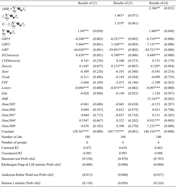
Estimation results with industrial structure similarity matrix are presented in Table 2. The first column reports results for linear strategic interaction as specified in (1); the second column reports results for asymmetric strategic interaction as specified in (3); and the third column

reports results for nonlinear strategic interaction as specified in (4). In all 2SLS regressions, models with random effects are preferred. Test statistics show that our specifications are fitted: the null hypothesis of underidentified instruments and the null hypothesis of the absence of endogeneity are rejected at 5%; the null hypothesis of overidentified instruments cannot be rejected at 5%.

Table 2: Strategic interaction with industrial structure similarity matrix

Results of (1) Results of (3) Results of (4)

it ijt j i

IMB Y

≠

∗

_∑

it ijt j i

I Y

≠

∑

(1 _it) _ijt j i

I Y

≠

−

_∑

ijt j i

Y

≠

∑

GRP3 -0.240*** (0.002) -0.221*** (0.003) -0.310*** (0.000) GRP2 5.664*** (0.001) 5.168*** (0.003) 7.151*** (0.000) GRP -44.020*** (0.001) -39.891*** (0.002) -54.721*** (0.000) SO2intensity 0.438*** (0.001) 0.398*** (0.000) 0.449*** (0.000) CODintensity 0.141 (0.230) 0.100 (0.273) 0.151 (0.178) Density 0.144* (0.057) 0.153*** (0.007) 0.128* (0.094) State -0.509 (0.226) -0.191 (0.580) -0.543 (0.214) Trade -0.211 (0.486) -0.145 (0.584) -0.099 (0.739) FDI -2.668 (0.189) -2.472 (0.146) -2.290 (0.265) Letters -0.094*** (0.000) -0.073*** (0.002) -0.097*** (0.000) Edu -0.028 (0.988) -0.149 (0.922) 1.136 (0.567) IMB 13.143** (0.042) Dum2005 -0.041 (0.688) -0.042 (0.638) -0.123 (0.287) Dum2006 0.049 (0.547) 0.012 (0.875) 0.031 (0.706) Dum2007 0.044 (0.712) -0.037 (0.710) 0.131 (0.265) Dum2008 0.554* (0.067) 0.323 (0.202) 0.931*** (0.005) Dum2009 0.676 (0.102) 0.390 (0.270) 1.231*** (0.008) Constant 120.567*** (0.000) 105.775*** (0.001) 146.316*** (0.000) Number of obs 180 180 180 Number of groups 6 6 6 Centered R2 0.472 0.636 0.463 Uncentered R2 0.985 0.993 0.988

Hausman test Prob>chi2 (0.338) (0.076) (0.783)

Kleibergen-Paap rk LM statistic Prob>chi2 (0.000) (0.000) (0.000)

Anderson-Rubin Wald test Prob>chi2 (0.013) (0.000) (0.037)

Hansen J statistic Prob>chi2 (0.110) (0.056) (0.216)

Note: Heteroscedastic-consistentp-value in parentheses, with ***, ** and * denoting respectively significance at 1, 5 and 10

Obviously, strategic interaction among provinces with similar industrial structure is much stronger and more significant than what was found among contiguous neighbors. When linear effect is considered, estimation results of equation (1) show that everything else being equal, a province would decrease (increase) its own environmental levy per industrial added value by 1.947% if its weighted competitors decrease (increase) theirs by 1%. The null hypothesis of zero strategic interaction can be rejected at the confidence level of 5%. These results suggest that environmental regulation stringencies of industrial competitors are effectively strategically determined.

When equation (3) is estimated, results reported in the second column don’t show evidence of asymmetric responsiveness. According to the race to the bottom theory, only the

coefficient of _{it jt}

j i

I Y

≠

∑

coefficients of _{it jt}

j i

I Y

≠

∑

I Y

≠

−

∑

This finding suggests that, no matter whether a province’s environmental stringency is stricter or not than its competitors, strategic interaction is not asymmetrically differential as predicted by the race to the bottom theory.7

Finally, estimation results of the nonlinear effects model (4) are reported in the last column. Consistent with the prediction in section 3, the interactionWWWWijtijtijtijtY_jt∗IMB_ithas a positive

and significant coefficient of 2.106, which suggests that strategic interaction among provinces is conditional on provincial fiscal imbalance. The more a province is fiscally dependent on central government’s transfers for expenditure, the more strategically it will set its environmental stringency vis-à-vis its competitors. These results are helpful to understand the potential inefficiency of China’s actual fiscal decentralization system for public good provision, especially in the environmental protection domain. Marginal effects of

competitors’ environmental stringency conditional on fiscal imbalance are presented in Appendix 4. Over the period 2004-2009, the province which has the strongest strategic interaction would be Qinghai, with a mean marginal effect of 3.688; the province which has the weakest strategic interaction would be Beijing, with a mean marginal effect of 2.233. In other words, everything else being equal, a decrease (an increase) of 1% in environmental stringency of their competitors would induce Qianghai and Beijing to decrease (increase) their own environmental stringency by 3.688% and 2.233%, respectively. It is notable that the significant nonlinear effects suggest that our strategic interaction is indeed driven by capital competition rather than pollution spillovers. The reason is that severe fiscal pressure can create strong incentives to attract mobile resources but has little to do with transboundary pollution problems.

Concerning control variables, GRP per capita, its squared and cubed terms have significant coefficients in all regressions. Population density has always a positive and significant coefficient, suggesting that everything else being equal, environmental stringency is stricter where it is more populated. In addition, complaint letter number has always a negative and significant coefficient, suggesting that public pressure weakens environmental stringency. This seems against intuition but is not surprising: public pressure of a province and its environmental stringency may be simultaneously affected. It is normal that stricter environmental stringency leads to fewer complaints. Given that complaint letter number is only a control variable, we don’t address its endogeneity in this paper.

5.

5.5.5. Conclusion:Conclusion:Conclusion:Conclusion:

Critics of decentralization often argue that capital competition and strategic interaction among jurisdictions in environmental regulatory enforcement may lead to inefficiently weak stringency and excessive pollution. Although this subject has been extensively studied in the U.S. context, very little attention has been given to the case of China. This paper contributes

to the environmental federalism literature in addressing the question of whether Chinese provinces engage in strategic environmental policymaking.

More specifically, we study whether Chinese provinces set strategically their environmental stringency vis-à-vis their competitors for mobile economic investment. It seems to us that this capital-competition driven strategic interaction is high likely to exist because, on one hand, Chinese central government has created a economic-performance based yardstick competition among local officials thus a strong local political incentive to attract investment; on the other hand, environmental policy implementation is largely decentralized, which endows Chinese local governments de facto authority of environmental stringency

enforcement and the possibility to use it as investment-attracting instrument. Using Chinese provincial data and spatial panel econometric methods, we find that Chinese provinces do engage in strategic interaction when they set their pollution levy. Moreover, this strategic interaction is particularly strong among provinces with similar industrial structure (i.e., potential competitors for attracting mobile capital). Furthermore, we haven’t found evidence of asymmetric responsiveness suggested by the race to the bottom theory. Provinces respond strategically no matter whether they are at an advantage or a disadvantage. Finally, the one-sided fiscal decentralization arrangements may strengthen strategic interaction.

Our empirical results in Chinese context lead us to take a skeptical attitude about the decentralization of environment policy implementation in this country. The strategic interaction among provinces driven by capital competition could be one of the reasons for China’s severe environmental degradation. Meanwhile, it is notable that the positive interaction also suggests a possibility to improve the whole environment beginning by some pilot regions. After all, it would be of great importance to develop more appropriate institutions for environmental protection and resource allocation in China, in paying more attention to both vertical and horizontal interjurisdictional relations.

Notes NotesNotesNotes

1. Abbreviations of three federal pollution control programs: the Clean Air Act (CAA), the Clean Water Act (CWA), and the Resource Conservation and Recovery Act (RCRA). 2. Different indices have been proposed in the literature to estimate structure similarity

between economies (Brixiova et al., 2010; Krugman, 1991; Landesmann and Szekely, 1995; UNIDO, 1979). In this paper, we utilize the index proposed by UNIDO (1979). More details on the construction of this index can be found in Appendix 1.

3. The race to the bottom theory suggests also another asymmetric pattern: a jurisdiction responds only if the weighted average of its competitors' environmental enforcement efforts drop from the previous year (Konisky, 2007). We haven’t tested for this model because quasi total observations in our sample have decreasing pollution levy over the period 2004-2009.

4. Following the GFS indicator, IMB doesn’t distinguish conditional transfers versus general purpose transfers, due to data unavailability.

5. The “composition” effect refers to the way that trade liberalization changes the mix of a country’s production towards those products where it has a comparative advantage.

6. The contiguity matrix with equal weights is not time-variant.

7. In the U.S. context, Fredriksson and Millimet (2002) and Konisky (2007) haven’t found asymmetric effects suggested by the race to bottom theory neither.

References ReferencesReferencesReferences

Anselin, L. (1988) Spatial econometrics: methods and models, Dordrecht, The Netherlands:

Kluwer Academic Publishers.

Anselin, L., Bera, A., Florax, R. & Yoon, M. (1996) Simple diagnostic tests for spatial dependence,Regional Science and Urban Economics, 26(1), 77-104.

Brixiova, Z., Morgan, M. & Worgotter, A. (2010) On the road to euro: how synchronized is Estonia with the euro zone? The European Journal of Comparative Economics, 7(1),

203-227.

Brueckner, J. (2003) Strategic interaction among governments: an overview of empirical studies,International Regional Science Review, 26(2), 175 -188.

Brueckner, J. & Saavedra, L. (2001) Do local governments engage in strategic property-tax competition?National Tax Journal, 54(3), 231-253.

Buettner, T. (2001) Local business taxation and competition for capital: the choice of the tax rate,Regional Science and Urban Economics, 31(2-3), 215-245.

Case, A., Rosen, H. & James R. (1993) Budget spillovers and fiscal policy interdependence: Evidence from the states,Journal of Public Economics, 52(3), 285-307.

Cole, M. & Elliott, R. (2003) Determining the trade–environment composition effect: the role of capital, labor and environmental regulations, Journal of Environmental Economics and Management, 46(3), 363-383.

Crone, T. (1998) Using state indexes to define economic regions in the U.S., Journal of Economic and Social Measurement, 25(3/4), 259-275.

Dasgupta, S., Laplante, B., Mamingi, N. & Wang, H. (2001) Inspections, pollution prices, and environmental performance: evidence from China, Ecological Economics, 36(3),

487-498.

Dean, J., Lovely, M. & Wang, H. (2009) Are foreign investors attracted to weak environmental regulations? evaluating the evidence from China, Journal of Development Economics, 90(1), 1-13.

Dijkstra, B. (2003) Direct regulation of a mobile polluting firm, Journal of Environmental Economics and Management, 45(2), 265-277.

Elhorst, J. (2010) Spatial panel data models, in M. M. Fischer & A. Getis (eds) Handbook of applied spatial analysis, Berlin, Heidelberg: Springer Berlin Heidelberg, pp. 377-407.

Figlio, D., Kolpin, V. & Reid, W. (1999) Do states play welfare games? Journal of Urban Economics, 46(3), 437-454.

Fredriksson, P. & Millimet, D. (2002) Strategic interaction and the determination of environmental policy across U.S. states,Journal of Urban Economics, 51(1), 101-122.

policymaking with multiple instruments, Regional Science and Urban Economics,

34(4), 387-410.

Fredriksson, P., Mani, M. & Wollscheid, J. (2006) Environmental federalism: a panacea or Pandora’s box for developing countries? Policy Research Working Paper 3847, the

World Bank, Washington.

Glazer, A. (1999) Local regulation may be excessively stringent,Regional Science and Urban Economics, 29(5), 553-558.

Hayek, F. (1945) The use of knowledge in society, The American Economic Review, 35(4),

519-530.

He, J. (2006) Pollution haven hypothesis and environmental impacts of foreign direct investment: The case of industrial emission of sulfur dioxide (SO2) in Chinese provinces,Ecological Economics, 60(1), 228-245.

Kelejian, H. & Prucha, I. (1998) A generalized spatial two-stage least squares procedure for estimating a spatial autoregressive model with autoregressive disturbances, Journal of Real Estate Finance and Economics, 17(1), 99-121.

Konisky, D. (2007) Regulatory competition and environmental enforcement: is there a race to the bottom?American Journal of Political Science, 51(4), 853-872.

Krugman, P. (1991)Geography and trade, MIT Press.

Kunce, M. (2004) Centralized versus local environmental standard setting: firm, capital, and labor mobility in an interjurisdictional model of firm-specific emission permitting,

Environmental Economics and Policy Studies, 6(1), 1-9.

Kunce, M. & Shogren, J. (2007) Destructive interjurisdictional competition: firm, capital and labor mobility in a model of direct emission control, Ecological Economics, 60(3),

543-549.

Kunce, M. & Shogren, J. (2002) On environmental federalism and direct emission control,

Journal of Urban Economics, 51(2), 238-245.

Kunce, M. & Shogren, J. (2005) On interjurisdictional competition and environmental federalism,Journal of Environmental Economics and Management, 50(1), 212-224.

Landesmann, M. & Szekely, I. (1995) Industrial restructuring and trade reorientation in Eastern Europe, Cambridge Books.

Levinson, A. (1997) A note on environmental federalism: interpreting some contradictory results,Journal of Environmental Economics and Management, 33(3), 359-366.

Levinson, A. (2003) Environmental regulatory competition: a status report and some new evidence,National Tax Journal, 56(1), 91-106.

Li, H. & Zhou, L. (2005) Political turnover and economic performance: the incentive role of personnel control in China,Journal of Public Economics, 89(9-10), 1743-1762.

Madariaga, N. & Poncet, S. (2007) FDI in Chinese cities: spillovers and impact on growth,

The World Economy, 30(5), 837-862.

Markusen, J., Morey, E. & Olewiler, N. (1995) Competition in regional environmental policies when plant locations are endogenous,Journal of Public Economics, 56(1),

55-77.

Martinez-Vazquez, J., Qiao, B. & Zhang, L. (2009) The role of provincial policies in fiscal equalization outcomes in China,The China Review, 8(2).

Maskin, E., Qian, Y. & Xu, C. (2000) Incentives, information, and organizational form, The Review of Economic Studies, 67(2), 359 -378.

Oates, W. (1999) An essay on fiscal federalism, Journal of Economic Literature, 37(3),

1120-1149.

Oates, W. (1972)Fiscal federalism, Harcourt Brace Jovanovich.

Oates, W. & Portney, P. (2003) The political economy of environmental policy, in: K-G Mäler, J R Vincent (eds), Handbook of Environmental Economics, Elsevier, pp.

325-354.

Oates, W. & Schwab, R. (1988) Economic competition among jurisdictions: efficiency enhancing or distortion inducing?Journal of Public Economics, 35(3), 333-354.

OECD (2006) Environmental compliance and enforcement in China: an assessment of current practices and ways forward, Paris: Organisation for Economic Co-operation

and Development.

UNIDO (1979) World industry since 1960: progress and prospects, special issue of the

Industrial Development Survey for the third General Conference of UNIDO, New Delhi, India, 21 January-8 February, 1980, United Nations.

Qian, Y. & Xu, C. (1993) Why China’s economic reforms differ: the M-form hierarchy and entry/expansion of the non-state sector,The Economics of Transition, 1(2), 135-170.

Revelli, F. (2005) On spatial public finance empirics, International Tax and Public Finance,

12(4), 475-492.

Roelfsema, H. (2007) Strategic delegation of environmental policy making, Journal of Environmental Economics and Management, 53(2), 270-275.

Tiebout, C. (1956) A pure theory of local expenditures,Journal of Political Economy, 64.

Wang, H. & Di, W. (2002)The determinants of Government environmental performance - an empirical analysis of Chinese townships, Policy Research Working Paper 2937, The

World Bank, Washington.

Wang, H. & Wheeler, D. (2003) Equilibrium pollution and economic development in China,

Environment and Development Economics, 8(3), 451-466.

pollution levy system, Journal of Environmental Economics and Management, 49(1),

174-196.

Wang, H., Mamingi, N., Laplante, B. & Dasgupta, S. (2003) Incomplete enforcement of pollution regulation: bargaining power of Chinese factories, Environmental & Resource Economics, 24(3), 245-262.

Wellisch, D. (1995) Locational choices of firms and decentralized environmental policy with various instruments,Journal of Urban Economics, 37(3), 290-310.

Wilson, J. (1986) A theory of interregional tax competition, Journal of Urban Economics,

19(3), 296-315.

Woods, N. (2006) Interstate competition and environmental regulation: a test of the race-to-the-bottom thesis,Social Science Quarterly, 87(1), 174-189.

World Bank (2002) China: National development and sub-national finance: a review of provincial expenditures, Poverty Reduction and Economic Management Unit, East

Asia and Pacific Region, The World Bank, Washington.

World Bank (2000) World development report 1999-2000: entering the 21st century, The

World Bank, Washington.

Wu, Y. (2010) Regional environmental performance and its determinants in China, China & World Economy, 18, 73-89.

Appendix 1: Industrial structure similarity index (UNIDO, 1979)

In order to construct our Industrial structure similarity matrix, we use the industrial structure similarity index proposed by UNIDO (1979). This index can be calculated as follows:

1 2 2 1 1 , n ikt jkt k ijt n n ikt jkt k k X X S X X = = = =

∑

∑

∑

where i and j denote provinces, t denotes the year, Sijt is the industrial structure similarity

index between province i and province j, k denotes the industry, Xikt and Xjkt denote the

employment number (or added value) in (created by) industry k in provinces i and j,

respectively. Sijt has a value between zero and one and increases with the similarity level

between province i and province j. Sijttakes the value “one” when province i and province j

have exactly the same industrial structure. In this paper, default of sectorial added value data in several years, we calculte Sijt with employment data of 27 industrial sectors published in

China Industrial Economic Statistical Yearbook (2005-2010). These 27 sectors are: production and supply of electric power and heat power, manufacture of electrical machinery and equipment, manufacture of textile wearing apparel, foot ware and caps, manufacture of textile, mining and processing of nonmetal ores, manufacture of nonmetallic mineral products, mining and processing of ferrous metal ores, smelting and pressing of ferrous metals, manufacture of chemical fibers, manufacture of raw chemical materials and chemical products, manufacture of transport equipment, manufacture of metal products, mining and washing of coal, processing of food from agricultural products, processing of petroleum, coking, processing of nuclear fuel, manufacture of foods, manufacture of beverages, manufacture of communication equipment, computers and other electronic equipment, manufacture of general purpose machinery, manufacture of tobacco, manufacture of medicines, manufacture of measuring instruments and machinery for cultural activity and office work, mining and processing of ferrous metal ores, smelting and pressing of non-ferrous metals, manufacture of paper and paper products and manufacture of special purpose machinery.

Appendix 2: Variable names and significations Variable names significations

Y Pollution levy per industrial added value (in log)

wY Spatially lagged Pollution levy per industrial added value (in log)

GRP Gross regional product per capita(USD at 2005 price, in log)

SO2intensity

SO2 emission per industrial added value (tons per 10000 USD at 2005 price, in log)

CODintensity

Chemical oxygen demand per industrial added value (tons per 10000 USD at 2005 price, in log)

Density Population density (persons per km2, in log)

State

Proportion of industrial added value created by state-owned enterprises

Open Ratio between the total trade and gross regional product

FDI

Ratio between actually used foreign direct investments and gross regional product

Letters

Number of complaint letters regarding environmental issues (in log)

Edu Percentage of population with high education

IMB Vertical fiscal imbalance indicator

Dum2005 1 if the year of 2005, 0 if not

Dum2006 1 if the year of 2006, 0 if not

Dum2007 1 if the year of 2007, 0 if not

Dum2008 1 if the year of 2008, 0 if not

Appendix 3: Summary Statistics

Variable Obs. Mean Standard Deviation Minimum Maximum

Y 180 0.002 0.001 0.000 0.009 GRP 180 2861.228 2075.915 511.462 11961.220 SO2intensity 180 0.233 0.215 0.017 1.150 CODintensity 180 0.058 0.072 0.001 0.547 Density 180 403.948 527.151 7.486 3029.969 State 180 0.451 0.191 0.059 0.834 Open 180 0.358 0.411 0.045 1.668 FDI 180 0.027 0.020 0.001 0.082 Letters 180 18231.950 19796.200 50.000 105942.000 Edu 180 0.072 0.050 0.025 0.289 IMB 180 0.520 0.185 0.141 0.930 Dum2005 180 0.167 0.374 0.000 1.000 Dum2006 180 0.167 0.374 0.000 1.000 Dum2007 180 0.167 0.374 0.000 1.000 Dum2008 180 0.167 0.374 0.000 1.000 Dum2009 180 0.167 0.374 0.000 1.000

Appendix 4: Nonlinear marginal effects conditional on IMB Overall 2004 2005 2006 2007 2008 2009 Mean 2.964 3.029 2.950 2.948 2.969 2.937 2.952 Minimum 2.165 2.300 2.262 2.241 2.187 2.165 2.203 Lower quartile 2.626 2.668 2.621 2.571 2.530 2.540 2.631 Median 3.078 3.129 3.063 3.067 3.111 3.078 3.045 Upper quartile 3.214 3.290 3.143 3.161 3.205 3.219 3.222 Maximum 3.827 3.827 3.759 3.637 3.623 3.674 3.605 S.D. 0.390 0.378 0.379 0 .378 0 .421 0.416 0.393 Observation number 180 180 180 180 180 180 180