Deployment of a next generation networking protocol

(1)

Deployment of a Next Generation Networking Protocol

by Logan Mercer

Submitted to the

Department of Electrical Engineering and Computer Science in Partial Fulfillment of the Requirements for the Degree of

Master of Engineering in Electrical Engineering and Computer Science at the

Massachusetts Institute of Technology May 2016 CS .. 10 Z

Author:

Signature redacted

Depa# ient of Electrical Engineering and Computer Science May 20, 2016

Certified by:

MASSARI SETTS INSTITUTE OFT CHNOLOGY

JUL

19 2016

LIBRARIES

Signature redacted

...

Tonas POicios, Associate Professor of Electrical Engineering May 20, 2016

Signature redacted

C ertified by: .. . . . . . . . . dreg Kuperman, Technical Staff, MIT Lincoln Lab

May 20, 2016

Acepe b:Signature

redacted

Accepted by: . Cis t re r ma ters ...

(2)

Deployment of a Next Generation Networking Protocol

by Logan Mercer

Submitted to the Department of Electrical Engineering and Computer Science On May 20, 2016

In Partial Fulfillment of the Requirements for the Degree of Master of Engineering in Electrical Engineering and Computer Science

Abstract

This thesis presents experimental verification of the performance of Group Centric Net-working (GCN), a next generation netNet-working protocol developed for robust and scalable

communications in lossy networks where users are localized to geographic areas, such as military tactical networks. In previous work, initial simulations in NS3 showed that GCN offers high delivery with low network overhead in the presence of high packet loss and high mobility. We extend this prior work to verify GCN's performance in actual over-the-air experimentation.

In the experiments, we deployed GCN on a 90-node Android phone test bed that was distributed across an office building, allowing us to evaluate its performance over-the-air on real-world hardware in a realistic environment. GCN's performance is compared against multiple popular wireless routing protocols, which we also run on our testbed. These tests yield two notable results: (1) the seemingly benign environment of an office is in fact quite lossy, with high packet error rates between users that are geographically close to one another, and (2) that GCN does indeed offer high delivery with low network overhead, which is in contrast to traditional wireless routing schemes that offer either high delivery or low overhead, or sometimes neither.

Thesis Supervisor: Tomas Palacios

Title: Associate Professor of Electrical Engineering

Thesis Supervisor: Greg Kuperman

(3)

Acknowledgements

I would like to thank Greg, Andy, and Brian, without whom this thesis would never have come together.

Funding Support: This work was supported by the Department of the Air Force under Air Force contract #FA8721-05-C-0002. Opinions, interpretations, conclusions and recommendations are those of the author and are not necessarily endorsed by the United States Government.

(4)

6 Link Quality 37 6.1 Beaconer. ... . . . .. .. ... .. .. ... 37 7 Over-the-Air Results 40 7.1 Summary of Results ... 40 7.1.1 D elivery . . . . 41 7.1.2 Resources Used . . . . 43 7.2 In-depth Results . . . . 46 7.2.1 C lique . . . . 46 7.2.2 C hain . . . . 47 7.2.3 One-to-Many . . . . 52 7.2.4 Many-to-One . . . . 57 7.2.5 Multi-rate Experiments. . . . . 63 8 Conclusion 70

(6)

Chapter 1 Introduction

With the desire to connect every soldier, vehicle, and sensor together via a battlefield intranet comes numerous networking challenges. Commercial networks enjoy fixed infrastructure with stable high-capacity links, as well as low mobility of users. These conditions enable a variety of network traffic patterns with little penalty for inefficient network use. Military tactical networks, however, operate under very different conditions: pre-existing infrastructure does not exist in the battlefield, connections are often low-rate and lossy, and soldiers and vehicles move rapidly in an ever-changing hostile landscape. Due to these fundamental challenges, robustly connecting users together in military tactical networks is still an open problem.

A similar problem is developing in the commercial world. The Internet of Things (IoT) [2] _{is the idea that every device, from the refrigerator to medical devices to automobiles, will} connect to one another. In a given location (house, factory, etc.), we expect 10s to 100s of devices to communicate with one another. Under this model, the amount of wireless traffic will skyrocket, and a single WiFi access point may not be able to process and coordinate all of the incoming data. Furthermore, much of this data is potentially destined for other devices operating in the same area, making the access point an unneeded bottle neck; those users can more efficiently communicate directly between themselves. Current wireless ad-hoc routing

(7)

schemes unfortunately do not scale well and have poor performance overall [12]. Because of this, there has been a large push to develop new schemes that can meet the challenges of the emerging IoT paradigm [13].

Tactical military networks and the Internet of Things highlight the new challenges that need to be addressed by future protocols; in particular, handling the amount of traffic, the number of devices, and the ad-hoc nature of the network. Group Centric Networking (GCN) is a proposed networking protocol that addresses challenges specific to military networks and IoT [8]. GCN operates by efficiently connecting users that share common interests within a certain geographic area. GCN moves from the address-centric model of networking, where devices send messages to explicit addresses in a client-server model, to a group-centric model where users that share a common set of interests communicate in a collaborative nature. This exploits the nature of the underlying network. For instance, in military networks, most communications are held within a local area and tend to exhibit collaborative traffic patterns (e.g., common operating picture, sensor fusion) as opposed to the client-server nature of more traditional networks [14, 11]. GCN offers the ability to scale to a large number of nodes because it efficiently connects interested users without flooding unneeded control information. Consider in the Internet of Things where an array of sensors are trying to communicate to some centralized controller. GCN allows these users to efficiently find one another and then to robustly exchange data.

When examining the success of a routing protocol, one must examine both the protocol's success at delivering packets and how many resources the protocols uses in the attempt. In highly dynamic networks, many wireless routing protocols send high amounts of control information while achieving only low delivery rates. Conversely, flooding protocols send little to no control information and can achieve high packet delivery, but at the expense of too much message redundancy that overloads the network. GCN aims to provide high delivery with low network load in lossy environments by balancing redundancy and control and taking

(8)

advantage of the wireless medium.

Prior to this work, GCN had only been evaluated in simulation. Here we explore the real-world performance of GCN on actual hardware, and compare its performance against several other ad-hoc routing protocols. We conduct our tests over-the-air on a 90-node Android phone test bed in an office environment. We find that GCN outperforms wireless unicast routing protocols by wide margins with respect to delivery ratio, and offers delivery rates comparable to flooding protocols while using as little as a third of the overall network resources. In addition, GCN also achieves higher delivery rates than flooding protocols in certain scenarios due to the flooding approach completely overwhelming network capacity. We also find that an office environment is in fact quite lossy, with users in close distance to

(9)

Chapter 2 Review of Protocols

In this chapter, we first provide a brief survey of the various routing schemes that we compare GCN against. We then present a brief overview of GCN.

2.1 Wireless Routing Protocols

In order to test the effectiveness of GCN, we compare against three other wireless routing protocols: Optimized Link State Routing (OLSR), Babel, and Simple Multicast Forwarding (SMF).

2.1.1 Optimized Link State Routing (OLSR)

OLSR is a proactive link state routing protocol where routes are continuously maintained between all users [6]. It is proactive in the sense that routes are continuously maintained such that a path exists to any destination when a user has data to send. This is in contrast to reactive protocols, such as Ad-hoc On-Demand Distance Vector (AODV) protocol [10] that finds paths in an on-demand fashion. In OLSR, every few seconds each node sends a neighbor list to its neighbors and a global topology view to the entire network. OLSR

(10)

employs multi-point relays (MPRs) to minimize the number of nodes retransmitting control messages. With a local and global view of the network, a node can determine and maintain a set of shortest paths between itself and all other users.

2.1.2 Babel

Babel is a loop-avoiding distance-vector routing protocol based on Destination-Sequenced Distance Vector Routing (DSDV) [4]. In a distance vector protocol, a node does not maintain paths to other users, but keeps track of which neighbor is the closest distance. This allows nodes to forward packets accordingly. It is a proactive routing protocol that uses the distributed Bellman-Ford algorithm to guarantee that no routing cycle is established between nodes. In the Babel protocol, nodes maintain several data structures to calculate paths.

2.1.3 Simple Multicast Forwarding (SMF)

Simple Multicast Forwarding (SMF) is a basic wireless flooding protocol [9]. In SMF, a message is transmitted with some time-to-live (TTL)1_{, and the message is rebroadcast by}

neighboring nodes. Each rebroadcast decrements the TTL until the TTL reaches zero. There is no control messaging in SMF - if a device hears a valid message with a nonzero TTL it will rebroadcast that message. The protocol uses duplicate detection to try to limit the number of packets transmitted, which works by checking received packets for the ID of the original sender as well as a packet sequence number. If a device has seen a message from that source with that sequence number before then it must be a duplicate and is thrown out. SMF seeks to achieve a high delivery rate at the cost of enormous data overhead.

1

Time-to-live is a method to prevent data from indefinitely circulating a network. It is implemented as a counter attached to a packet that is decremented every time a message is sent. TTL is also known as a hop limit.

(11)

0 ₀

0 b

0

0 0O

*

Group

0 Non-Group Relay

0 Non-Participating User

Figure 2.1: An example of a group centric network. Figure from [8].

2.2 Group Centric Networking

Group Centric Networking is a networking protocol designed to support groups of devices in a local region [8]. It attempts to use minimal control information to allow it to scale to very large numbers of nodes. Both unicast and multicast messaging are supported. GCN is organized around the concept of a group, which is a collection of devices in some geographic area that are interested in each others traffic. An example group centric network is presented in Figure 2.1. Groups can be formed on arbitrary subsets of nodes, and one node may be in many groups. To efficiently and robustly disseminate data, three major mechanisms are employed: Group Discovery, Tunable Resiliency, and Targeted Flooding. Group Discovery connects interested users together, and Tunable Resiliency and Targeted Flooding allow for robust traffic flow between these users. A brief description of each of the major mechanisms are presented; further details and analysis can be found in [8].

2.2.1 Group Discovery

The goal of the group discovery algorithm is to allow group nodes to find each other without globally flooding control messages. To facilitate this, GCN uses discovery regeneration, an

(12)

adaptation of the familiar Time-to-Live (TTL) approach. A description of the algorithm follows:

1. A node begins group discovery by sending out a message. This discovery message includes a low TTL.

2. If a group member hears the discovery message it rebroadcasts the message with the source TTL. The group node also sends an acknowledge message back to the most recent message sender. This ack will be used later to establish relays.

3. If a non-group member hears a discovery message it will decrement the TTL.

Non-group nodes will rebroadcast the message until the TTL reaches zero. Every time a group node hears a group discovery message it refreshes the TTL, effectively regenerating the discovery message, while non-group nodes only decrement the TTL. Thus the discovery message will only be heard by nodes near group nodes. This limits control messages to small (but tunable) geographic areas.

Data relays are elected by acknowledgement messages (ACK) sent in response to discovery messages. All nodes in between group nodes that receive an ACK are elected as data relays. Duplicate detection is used to ensure discovery messages are broadcast only once. Once a node is elected as a relay it acts as a relay for the entire group, not just the nodes it originally acknowledged. Nodes do not need to store any information about neighbors or to whom they sent ACKs. At the end of the group discovery algorithm each group node has a path to any other group node, thus enabling a one-to-many (multicast) traffic pattern.

An example of group discovery with regeneration is shown in Figure 2.2. Each arrow shows the time-to-live (TTL) of the outgoing discovery message. The source node starts Group Discovery with a TTL of 2. At transmission this value is decremented to 1, and group members regenerate the TTL at the source value of 2. Non-group members do not regenerate

(13)

0 0

1

0

1

0

a

0

0 Initiating Group Member

0 Group

0 Non-Group

Figure 2.2: Discovering the local region using discovery regeneration. Each arrow shows the time-to-live (TTL) of the outgoing discovery message. Figure from

[8].

the TTL, which limits the reach of the discovery message to the local region where group members reside.

2.2.2 Tunable Resiliency

Tunable resiliency is a mechanism to activate additional relays during the group discovery process. Group discovery will create a minimal spanning tree between group nodes, but a

single failure will potentially disconnect the network. To increase resiliency, group discovery

is extended to have devices probabilistically self-select as data relays.

When a node enters the network it enters with a preset resiliency parameter R, with

group discovery messages containing this parameter. This parameter represents the number of neighbors this node desires to have as relays. After group discovery, one node is selected

as an obligate relay. An additional R - 1 nodes need to be activated as relays. If a node

has N neighbors, it sets the probability its neighbors become relays to

y-}.

Each neighbor opts into becoming a relay with that probability, so a node has on average R relays in its

(14)

0

000

0

(a) Minimumn set of relays to connect the group

0 ₀

0000

₀

(b) Mimore relays allow resilient group communications

40Group oGroup 0Non-Group 10Non-Group

WReceive and Relay Receive Only Relay Non-Participating

Figure 2.3: Change in coverage using tunable resiliency. Figure from [8] neighborhood.

GCN's Tunable Resiliency allows the network to increase redundancy by allowing nodes to self-select as redundant relays and thus perform well in lossy networks in an efficient manner. Figure 2.3 shows an example of tunable resiliency. In Fig 2.3a, the minimum set of relays is activated and the entire group is connected. When a group member sends a transmission, all of the group members will receive the message. But, if any packet is lost, or any relay moves out of range, then the group will become disconnected. In Figure 2.3b, additional relays have been activated by setting the R value in the ACK message to achieve the target number of relays. This allows data to cover more of the group area, which increases the

(15)

resiliency of the group against packet loss and mobility.

2.2.3 Targeted Flooding

We have so far discussed Group Centric Networking's one-to-many communications, but GCN also includes an effective way to send data one-to-one (unicast) via a "targeted flooding" mechanism. Targeted flooding uses distance information gathered from overheard packets to create a distributed gradient field towards each of the group members. Then, when a user wants to send data to another it simply forwards the packet in the direction of the distance gradient. GCN does not record any information about particular links or neighbors, it simply maintains this distance gradient.

To increase the resiliency of Targeted Flooding, GCN can opt to send duplicate packets towards less optimal gradient routes. With no resiliency GCN only sends a single packet along the most likely distance gradient, but with higher resiliency other packets will be sent to try to reach the destination. To create a many-to-one traffic pattern (such as a set of sensors), each of the many nodes can establish a one-to-one connection with a sink node.

(16)

Chapter 3 Development and Compiling

3.1 Building GCN for Android

Originally, GCN was developed for the Unix operating system, and in particular was targeted for Ubuntu Linux. Though GCN is written in C++, which generally results in code that is portable across platforms, there were significant challenges to compiling and executing it on the Android operating system. The main difficulties lay in obtaining the correct software to allow for cross compilation, determining the changes to be made to the build process, and porting all of the dependencies needed by GCN to Android, as GCN is not a completely standalone application.

Cross compilation from Ubuntu to Android begins by setting up the necessary environ-ment. We began by downloading the Android Software Development Kit (SDK) and Native Development Kit (NDK). The SDK is necessary to compile any Android program. The NDK allows g++ to compile an Android application that uses C and C++ code. Without the NDK, Android applications can only be written in Java.

Cross compiling is creating executable code for a platform other than the one on which the compiler is running. Android devices cannot compile Android code, so in order to create an

(17)

Android application one has to cross compile it from some other machine (Linux, Windows, OS X). For our build, we used a Linux machine to make the application. g++ was given the Android toolchains in order to make a program that would run on Android.

Next, a few changes to the normal GCN build process are necessary. GCN was built using CMake, a program designed to help automate building and packaging software. CMake takes a few CMake build files and automatically generates appropriate makefiles and workspaces for any compiler environment. In order to compile GCN for Android we had to change several CMake flags, including setting the cmake-cxx-compiler to arm-linux-androideabi-g++, setting the cmake-c-compiler to arm-linux-androideabi-gcc, and setting the cmake-install-prefix to the android-ndk toolchain.

Finally, all of GCNs dependencies needed to be ported to Android in order to allow it to run. Boost, Google Protocol Buffers, and libpcap are all required for GCN. However, these are not native to Android, and themselves need to be correctly set up in order to function properly in a new operating system. Though dynamic linking, in which necessary libraries are linked to the executable at runtime, is a possibility, statically linking these libraries, which is when libraries and dependencies are compiled into the executable, greatly simplified the build and distribution process.

Additionally, the resulting GCN software was targeted to only a specific phone, the Samsung Galaxy S4 running Cyanogenmod 10. Other phones, especially those with different versions of the Android operating system, could require different steps in the compilation

process.

The end result of this process is an application that runs on the phones. It has a basic command line interface that takes parameters at run time. When a device launches the GCN application it indicates which group it wants to join, if it intends to send traffic, receive, or both, how frequently it wants to initiate the Group Discovery algorithm, its desired message resiliency, and many more system parameters.

(18)

Chapter 4 Test Setup

In order to compare GCN against the other routing protocols in real networks on real devices, we compiled and tested OLSR, Babel, GCN, and SMF on a network of 90 Android phones in

an office environment.

4.1 Android Phones

As mentioned earlier, the Android phones are Samsung Galaxy S4 running Cyanogenmod 10.2. For the network, we use 802.11ac WiFi running in the 5GHz band and using a transmit power of 1 mW. All transmissions occur via 802.1lac broadcast mode, which has no acknowledgement packets and runs at a fixed rate of 6 Mbps [7]. We purposely choose to transmit via broadcast mode in order to avoid any MAC layer features that may not exist in other networks, such as MAC layer retransmits and rate adaptation. Furthermore, by limiting the MAC to be a simple broadcast, we are better able to evaluate the network layer protocols.

In order to generate traffic for OLSR and Babel, the devices run Multi-Generator (MGEN) [3]. GCN is built with its own traffic generation for testing purposes.

(19)

a

C

e

b

d

f

Figure 4. 1: Chain Topology

4.2 Topologies

We tested the devices in three topologies to get an understanding for how they would behave. We tested them in a clique, a chain, and an office.

4.2.1 Clique

In a Clique every device is fully connected to every other device. Unfortunately, due to WiFi limitations, we were only able to explore cliques smaller than 20 devices.

4.2.2 Chain

The chain topology is a linear topology in which devices can communicate well with their immediate neighbors. The chain topology is more controlled than the office topology so it is easier to see where traffic is going and coming from. It is more interesting to observe than a clique as it has many hops in the network. We test this topology for networks of size 9 to 60 devices, so we explore networks of diameter 3 to 20.

A diagram showing the chain topology can be found in Figure 4.1. In this diagram node (a) and node (b) form a pair, and that pair is fully connected with the pair (c) and (d). Similarly, (c) and (d) can communicate with (e) and (f), and so on.

y

z

(20)

Figure 4.2: Office Topology

4.2.3 Office

We tested the routing protocols over several topologies within an office building with varied layouts and densities to understand their performance. The office floor plan is shown in Figure 4.2.

Phones are distributed with approximately 1 to 3 phones per room, resulting in a large network diameter. In this topology there can be many paths from one node to another. In order to vary network density, we test this topology with 30, 60, and 90 nodes spread over the same area. This topology is meant to be stressing and is realistic in that it is very similar to the actual distribution of smartphones found in those offices during normal working hours.

4.3 Traffic Patterns Tested

4.3.1 One-to-Many

The one-to-many traffic patterns test routing protocols in a typical server/client fashion. In a one-to-many test there is a single source node and many receiver nodes. 25% of the devices are designated as group members interested in receiving data from the source node. The source node then sends broadcast traffic to each of the receivers.

This traffic pattern is similar to classic multicast patterns, which are often seen in military tactical networks [14]. Voice traffic and situational awareness are typically transmitted via a

(21)

one-to-many traffic pattern.

4.3.2 Many-to-One

In the many-to-one traffic pattern we run the same experiment as above, but each receive node generates and sends a message back to the source. This traffic pattern tests the network under much heavier conditions since each group member now is a source for packets.

This traffic pattern models a case in which sensors are distributed throughout a network with a single processing unit that wants to aggregate data from the sensors. The processing unit sends commands to the sensors and the sensors send back what data they have collected.

(22)

Chapter 5 Simulation and Emulation

5.1 Simulation Results for GCN

Prior to this work, extensive simulations were run to measure the performance of GCN. A full explanation of this work can be found in [81. In particular, GCN was simulated in Network Simulator 3 (NS3), with comparisons to SMF and Ad-Hoc On-Demand Distance Vector (AODV) routing [10] (which is another commonly used wireless routing protocol). Networks of 50 and 100 users were compared, and performance was examined under realistic packet error rate curves.

In those simulation results, GCN significantly outperformed AODV with respect to delivery and outperformed SMF with respect to efficiency. In particular, in high loss environments, GCN delivered 97% of traffic while AODV delivered between 6% and 12%. Since SMF is a flooding protocol, it was able to deliver close to 100% of packets in this scenario; however, GCN transmited an order of magnitude fewer packets to achieve a similar delivery rate. We also note that the data links in NS3 had no capacity limits, which allowed SMF to transmit as much data as it desired between any pair of users.

(23)

5.2 Emulating GCN in EMANE

Before launching experiments over WiFi, we used the Extendable Mobile Ad-hoc Network Emulator (EMANE) [1] to get an understanding and a baseline performance of GCN on the Android phones. EMANE is a framework for real-time modeling of mobile network systems [5]. It creates a virtual network for devices to communicate, and it gives us complete control of the devices' network conditions. EMANE is a useful because it will behave exactly as the parameters dictate - there is no external interference, and repeating a test multiple times will yield the exact same result. We created an EMANE environment that matches the Chain topology discussed in Section 4.2.2. We then ran experiments of size 9, 18, 30, 45, and 60 nodes.

The Android phones connected to an EMANE server by USB cable. The phones were given different traffic patterns and ran GCN, SMF, and OLSR over EMANE as if it were a network connection. In the following sections we review different EMANE tests performed on the devices. We will compare these results to the results from simulation as well as to other EMANE results.

We include these results in part because they demonstrate the importance of doing actual over-the-air tests. When examining EMANE results we will find trends in the routing protocols that continue in over-the-air tests. However, results in EMANE can misrepresent a protocol's actual performance. Over-the-air connections suffer external interference and unpredictability. Each over-the-air link between devices is not exactly identical to the next, and these realistic differences in connectivity add up to a huge difference in network performance. EMANE gives us a great first cut at the performance of each protocol, but real over-the-air networks will behave differently. It is important to run over-the-air tests to understand how a protocol will actually behave in a real scenario.

(24)

100.00% 90.00% 80.00% 70.00% > 60.00% C 50.00% U 40.00% 0- 30.00% 20.00% 10.00% 0.00%

Res 0,0 Res 0,1 Res 0,2 Res 3,0 Res 3,1 Res 3,2 Res 6,0 Res6 1 Res 6,2 SMF OLSR

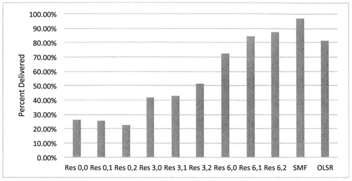
Figure 5.1: EMANE 9 Node Experiment, Percentage of Packets Delivered, Many-to-One

5.2.1 9 Node Emulation

The first set of experiments run for this paper used 9 devices over EMANE. The devices were configured in a chain topology, so devices 1, 2, and 3 could only communicate with 4, 5, and 6. Devices 7, 8, and 9 could also communicate with only 4, 5, and 6. The middle devices could hear everyone. There were only two hops in this network, so devices 4, 5, and 6 relayed to help 1, 2, 3 communicate with 7, 8, 9. A graph of the results can be found in Figures 5.1 and 5.2.

In these figures we provide data on every GCN parameter we used. In GCN, the first resiliency number is the resiliency used in Group Discovery that creates obligate relays. The second is the resiliency for Targeted Flooding, GCN's unicast mechanism. For example, Res 0,2 means GCN was run with one-to-many resiliency parameter of 0 and with a unicast resiliency of 2. In future sections we will simplify the GCN results to two resiliency levels, denoted GCN Low and GCN High. GCN Low will refer to Res 3,1 and GCN High will refer to Res 6,1. We use these values because a resiliency lower than 3 does not create a stable

(25)

connection between all of the group nodes, and generally nodes to not have enough neighbors to take advantage of a resiliency larger than 6.

In Figure 5.1 we can clearly see that increasing the GCN resiliency increases the percentage of packets delivered. This is because increasing resiliency makes more nodes obligate relays, so more nodes can relay packets. The higher redundancy in the network increases the percentage of packets delivered.

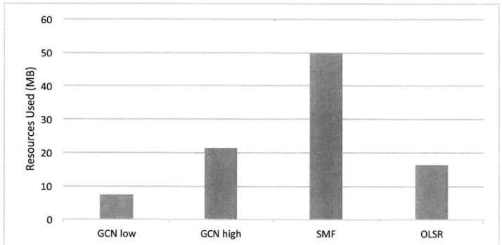
In Figure 5.2 we see the total resources used in the experiment. This is the total number packets sent through EMANE, including control packets and data packets. Increasing GCN resiliency tends to increase the data used because more nodes are obligated into sending the data.

Compared to GCN, SMF delivers more packets and uses more data. SMF floods the network with data packets, so it is not surprising that it uses so much data. We will see in our over-the-air tests that the flooding approach overwhelms the network, and that for larger test cases, SMF does not perform well.

OLSR is significantly more efficient than SMF is, but it does not deliver as many packets. In this small EMANE example OLSR looks about as good at delivery as GCN on a high resiliency rating. This small 9 node chain is very favorable for OLSR, but we will see it struggle to deliver data as the diameter of the network increases.

5.2.2 18 Node Emulation

The next test we ran over EMANE used 18 nodes, twice as many as the first. Like before, nodes are grouped into triplets and can only hear adjacent triplets. The network now had a diameter of 5. A graph of the percentage of data delivered can be found in Figure 5.3. A graph of the resources used can be found in Figure 5.4.

Starting with this test we simplify the results to GCN Low and GCN High, meaning GCN with low and high levels of redundancy. Of course, GCN's resiliency exists on a continuum

(26)

3.5 3 2.5 (U _S2 L 1.5 1 0.5 0

Res 0,0 Res 0,1 Res 0,2 Res 3,0 Res 3,1 Res 3,2 Res 6 0 Res 6,1 Res 6,2 SMF OLSR

Figure 5.2: EMANE 9 Node Experiment, Network Resources Used, Many-to-One

so any set of resiliency values could be set to cater to a particular network. Like before, increasing the resiliency increased both the percentage of packets delivered and the data required to do so.

Interestingly, all of the routing protocols delivered a higher percentage of packets in this experiment than they did in the 9 node experiment. Consider Figures 5.1 and 5.3. We can attribute this increase to the increase in total redundancy in the network. Our EMANE model's link states were configured to match what we found over-the-air. That is, any two connected devices will drop 30% of the packets sent between each other to model real over-the-air conditions. When there were only 9 devices in the network, increasing GCN resiliency could only obligate so many extra devices to be relays, so there is a maximum cap

to the number of redundant packets sent in the network. Now that there are 18 devices there

is much more room for protocols to send redundant messages. As we increase to even more devices we will see SMF and GCN take advantage of the additional relays. It won't always lead to an increase in packets delivered, however, because with more devices comes more

(27)

Q) C 100.00% 90.00% 80.00% 70.00% 60.00% 50.00% 40.00% 30.00% 20.00% 10.00% 0.00%

GCN low GCN high SMF OLSR

recipients.

This increase in devices should not favor OLSR, but OLSR still performs well. As the networks get even larger we will see OLSR's performance decline. As is seen in emulation, the chain topology favors OLSR.

5.2.3 Larger Scale Emulation

Here we will discuss the results of the 30, 45, and 60 node tests.

30 Nodes

The 30 node network now has a diameter of 9, roughly twice the diameter of the 18 node network. The trends from the 18 node network are only furthered in the 30. The percentage of packets delivered in the 30 node network can be found in Figure 5.5. SMF, OLSR, and GCN on high resiliency all deliver an enormous number of packets.

(28)

18 16 14 12 O) (n 10 ZD 4 2 0

we see SMF use significantly more packets than the other protocols. In a tactical environment or in the Internet of Things it is likely that SMF would be an inappropriate choice for a 30 node network because it is so wasteful with the limited network resources. Additionally, SMF's resources used has increased significantly from the small 9 node tests, and we expect this trend to continue.

In this test case OLSR delivers almost as many packets as GCN does and it uses notably less data. This case is OLSR's highest performing result in the entire suite of tests run. We can attribute OLSR's success to the stability of the EMANE environment as well as the relatively small network size. Larger networks will cause OLSR to send more control data, and less stable networks will cause OLSR's links to fail.

45 Nodes

In the 45 node experiments we see an inflection point in our data. In the 9, 18, and 30 node experiments SMF used a significant amount of data but was most successful in delivering

(29)

100.00% 90.00% 80.00% -0 70.00% L. > 60.00% 50.00% a 40.00% 30.00% 20.00% 10.00% 0.00%

packets. In Figure 5.7 we see SMF deliver less than 50% of the data while OLSR and GCN on high resiliency both delivered above 60%.

This dip in performance happens because SMF hit the link capacity of the EMANE connection. That is, SMF's flooding approach filled the network with packets and induced collisions between devices. If we look at Figure 5.8 we see that SMF used twice as many bytes in the 45 node experiment as it did in the 30 node experiment. The other protocols' usage did not grow at this rate. SMF's enormous data consumption cannot be supported by the wireless links. We will see a similar inflection point in the over-the-air tests in the next chapter.

GCN and OLSR are able to maintain their delivery percentages in this experiment because they use significantly less data per packet delivered. SMF used 100MB in this experiment while GCN and OLSR each used less than 40MB.

(30)

60 50 40 D Ln 30 0 ~ U 10 0

GCN low GCN high SMF OLSR

60 Nodes

We made a few changes to the EMANE topology for the 60 node experiments. In the 45 node EMANE experiment SMF hit link capacity and so it was unable to deliver a significant percentage of the traffic. Continuing that trend to a 60 node chain would not reveal interesting results. For the 60 node topology we deviated slightly from the chain and opened a few more paths between devices. Now a triplet of nodes would have a 70% packet error rate when connecting to their immediate neighbors and a 30% packet error rate when communicating with devices two hops away.

For 60 devices we looked at both the many-to-one traffic pattern and just the one-to-many traffic pattern. The many-to-one pattern is the same as we saw in previous EMANE tests.

Many-to-One

In the Many-to-One traffic pattern with a modified Chain topology we see results similar to the 9, 18, and 30 node experiments. The percentage of packets delivered by each routing protocol can be found in Figure 5.9. With new pathways opened up SMF is able to deliver

(31)

100.00% 90.00% 80.00% 70.00% i 60.00% c)50.00% 4_j C w 40.00% U L_ 30.00% 20.00% 10.00% 0.00%

GCN Low GCN High SMF OLSR

100% of the packets. GCN and OLSR also do well in this topology.

It is interesting to compare the data used in this experiment to the 45 node experiment. Figure 5.10 has the 60 node experiment's data usage while Figure 5.8 has the 45 node's. We can see that SMF in the 60 node experiment uses significantly more data then the 45 node experiment does. Changing the topology slightly gave nodes more neighbors, so they were able to send more messages. Of course, some of this increase can be accounted for with the increase in group nodes.

One- To-Many

In the One-to-Many traffic pattern there is a single source node that packets sends to many recipients. Fewer packets are sent over the channel in this experiment because only a single node is sourcing them. Previously many group nodes would also send packets.

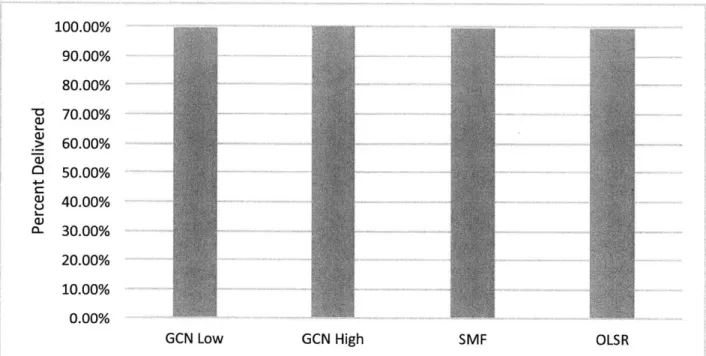
Since fewer packets are sent over the air, this traffic pattern is much less straining on the network. We can see the total percentage of packets delivered in Figure 5.11. All of the protocols delivered 100% of the data. The controlled environment provided by EMANE

(32)

120 100 2. 80 -a (U 60 Q) ai 20 0

combined with the redundancy of a well connected 60 node network allowed even GCN on low resiliency and OLSR to perform well.

Consider the resources used in Figure 5.12. This test case demonstrates the value of GCN's tunable resiliency. Both GCN on high resiliency and low resiliency deliver 100% of the data, but GCN on high resiliency uses three times the bytes to do so. In a lossy, contested environment where network bandwidth is limited it would make more sense in this example to use GCN on low resiliency.

From the graph we can see GCN using far fewer resources than SMF and OLSR. In previous Many-to-One examples OLSR tended to use around the same order of resources as GCN, so it is unusual to see it's usage spike so high. This relative change takes place because OLSR is a proactive network. No matter the number of packets OLSR is required to send it will send the same large amount of control information around the network to establish good links. GCN and SMF used much less data when they did not have to send many packets. OLSR, however, continued to flood the network even under light traffic conditions. We expect

(33)

100.00% 90.00% 80.00% 70.00% CU > 60.00% 50.00% U 40.00% a- . S30.00% 20.00% 10.00% 0.00%

this trend to continue, so in networks larger than 60 nodes OLSR would waste even more network resources.

5.2.4 Many-to-Many

We decided to try altering GCN after reviewing its performance in previous sections. In general, SMF used much more data than GCN but was able to deliver slightly more packets, particularly in low stress environments. In order to improve GCN's performance in these low stress environments we tested a version of GCN that behaved more like SMF.

In the many-to-one experiments half of the data sent is multicast traffic from a source to group nodes. The other half of the traffic is unicast traffic from the group nodes back to the original source. GCN and OLSR send unicast packets for the many-to-one data while SMF continues to broadcast packets to everyone. Devices in SMF that are not interested in the broadcast data simply ignore it. For just this experiment we altered GCN's targeted flooding protocol to use broadcast packets instead of unicast. Like in SMF, devices not interested in

(34)

200 180 160 140 z 120 U 100 :3 Ln80 60 40 20 0

a node's traffic would just ignore it. We intended this to slightly increase data usage but significantly improve the performance of the network.

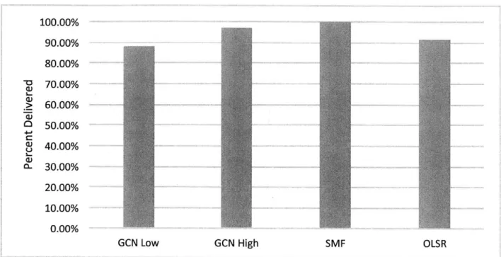
The effects of the change can be found in Figure 5.13. In the many-to-one 18 node test, found in Figre 5.3, SMF delivered almost all of the packets. The two resiliencies for GCN did not boast as high of a delivery rate. In particular GCN low delivered a little more than 70% of the data. Now GCN low delivers almost 90% of the traffic.

However, this increase in GCN performance comes at cost to the network bandwidth. From Figure 5.14 we can see that GCN on its low resiliency used almost 8MB while in the many-to-one experiment used less than 4MB. GCN on a High resiliency in the many-to-one test used over 9MB to deliver 99%, so we find that the many-to-many approach is not an efficient solutoin. It would simply be better to increase the resiliency of GCN rather than change the protocol in this case.

(35)

_0 4-J U 100.00% 90.00% 80.00% 70.00% 60.00% 50.00% 40.00% 30.00% 20.00% 10.00% 0.00%

GCN Low GCN High SMF OLSR

Figure 5.11: EMANE 60 Node Experiment, Percentage of Packets Delivered, One-to-Many

45 0) a) U 0 40 35 30 25 20 15 10 5 0

(36)

1~ w .4-I C a, C-) a, 0~ 100.00% 90.00% 80.00% 70.00% 60.00% 50.00% 40.00% 30.00% 20.00% 10.00% 0.00%

Figure 5.13: EMANE 18 Node Experiment, Percentage of Packets Delivered, Many-to-Many

18 16 14 12 10 8 a4 4 2 0

(37)

Chapter 6 Link Quality

6.1 Beaconer

Over-the-air experiments do not enjoy the consistency provided by simulation and emulation. Links between devices are widely variable over-the-air, and no two networks in different locations are going to be exactly the same. We examine the quality of links between devices in our topology to contextualize our results. An environment with more or less external interference would behave differently.

To evaluate the connectivity between devices, we wrote a lightweight program called Beaconer to collect link statistics. Beaconer broadcasts a 64 byte packet one hop every 3 seconds and records packet receptions of neighbors. By comparing the number of received Beaconer packets between userswith the number of transmitted Beaconer packets, we get estimates of packet error rates for particular links between users throughout experiments. Using this data and the locations of the phones, we created a Packet Error Rate (PER) vs. Distance graph for the different topologies. The average curve for data collected over all tests is shown in Figure 6.1.

(38)

100 80 60 0 4- 40 C-) 20 0 0 20 40 60 80 100 120 Distance (ft)

Figure 6.1: Observed packet error rate vs. distance between users

While some phones might have up to a dozen other phones within 30 feet, in reality, only few of those links are reliable. If we consider sub-graphs of the network that have only links of some minimum Beaconer success rate, we get a better picture of the reliable network topology. Figure 6.2 is a plot of the average node degree when links are limited to a maximum packet error rate (minimum Beaconer success rate) for a sample 60 node test. The 0% Beaconer success rate represents users that exchanged at least one Beaconer message, but not sufficient numbers to register a full percentage point. Users that exchange at least one message have

13 neighbors on average. With 50% Beaconer success rate, a node only has an average of 5

neighbors. For a 90% Beaconer success rate, a node can expect to have at most 1 neighbor, meaning that there are very few reliable links throughout the network.

Continuing with the sub-graph approach where only links that have a minimum Beaconer success rate are included, we consider the number of users that actually reach one another and the average path length between them. For the 0% Beaconer success rate, a path exists between all users, and the average distance between users is 3.6 hops. For 50% Beaconer success rate, only 34% of users are connected between one another, and the users that remain connected have an average distance of 4.4 hops between themselves. For 70% Beaconer

(39)

0

0i 14

12

10

8 6

4

2 0

-0% 25% 50% 75% 100%

Beaconer Success Rate

Figure 6.2: Average node degree of sub-graphs with links of a minimum Beaconer success rate

success rate, a meager 9% of users are connected. As shown by our tests, reliable paths between users unfortunately cannot be expected to exist.

These tests were conducted in an office with presumably negligible external interference and no mobility. Even in such a benign environment, the over-the-air links between nodes are very lossy. This demonstrates the challenges that the Internet of Things faces as it tries to connect 100's of nodes. A tactical network would see connectivity potentially even worse than this. The channel would be contested by other users and jammers, and we expect the nodes to be mobile.

(40)

Chapter 7 Over-the-Air Results

Now we look at the results of the tests run over the air. To measure performance, we look at what percentage of messages successfully delivered, as well as the total network load of packets transmitted over-the-air. While some protocols deliver a high percentage of packets, they do so at such a high cost that may not be supportable in heavily resource constrained environments.

The results section is organized as follows. We begin with a condensed section of hand-picked tests that best showcase the differences between the protocols. The next section will have an in depth analysis of each experiment run.

7.1 Summary of Results

Here we will look at a condensed representation of the results.

In these experiments, we test two resiliency levels for GCN: high and low. High resiliency sets the relay parameter R to 6, and low resilience sets R to 3. We note that these resiliencies exist on a continuum so they could be changed to meet the needs of the network.

(41)

100%

--) U )

80%

1 60%

40%

20%

0%

E30

node

-60

node

M

90 node

GCN

SMF

OLSR

Babel

Low

High

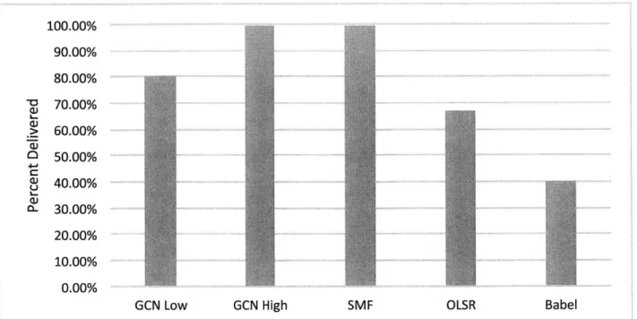
Figure 7.1: Percentage of Packets Delivered, One-to-Many

network density, not network diameter.

7.1.1 Delivery

One-to-Many

In the one-to-many traffic pattern a single source node is sending data to many receive nodes. One quarter of the devices are designated as receive nodes.

We have found the over the air results follow what we saw in NS3 simulation. GCN outperforms the other routing protocols. Figure 7.1 shows the percentage of packets delivered for the different routing protocols and parameters run. GCN at both low and high resiliencies was able to deliver 100% of the packets. Babel only managed to deliver half of the traffic and OLSR delivered between70% and 80%. Like GCN, SMF delivered 100% of the packets. Though SMF delivered packets successfully, we see in later sections that this success came at huge cost. GCN's success we can attribute to successful group discovery. Nodes in the

(42)

a-a)U3 4-, CL 100%

80%

60%

40%

20%

LI

0%

---]

_K

l 30 node

060 node

090 node

GCN

SMF

OLSR

Babel

Low

High

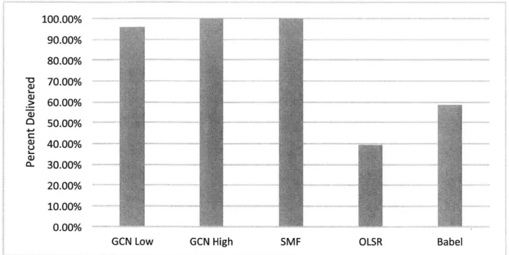
Figure 7.2: Percentage of Packets Delivered, Many-to-One

topology found each other and sent data back and forth successfully. OLSR and Babel often failed to establish links between participating devices and thus could not send data.

Many-to-One

The many-to-one traffic pattern is more demanding on all of the protocols. Now a quarter of the devices are active senders and they each want to deliver traffic to the same receive node. No protocol surveyed was able to deliver 100% of the required traffic.

As expected, SMF and GCN on high resiliency have the highest delivery rates. Interestingly, as network density increases, GCN performs at least as well while SMF's performance declines. At only 30 nodes SMF delivers over 80% of packets while GCN at high resiliency delivers 70%. As we move to 60 and then 90 nodes we see SMF's delivery rate decline to 60% and GCN's high resiliency performance stay the same. GCN on low resiliency performs even better as network density increases.

In a 30 node network, low resiliency GCN delivered only around 40% of the packets, but in a 90 node network, both low and high resiliency GCN performed similarly, delivering 70%

(43)

of the packets. This change is caused by the difference in node density. Under high density, there are many good links to choose from, resulting in high delivery, but in a sparse network, there may be only one good relay to choose. Low resiliency GCN has a low probability of choosing this good relay, whereas the increased number of relays selected by high resiliency GCN results in a much greater chance of selecting this good choice. The consequence of this higher likelihood of selecting the best relay is that high resiliency GCN uses significantly more network resources.

OLSR and Babel both could only deliver approximately 30% of packets to their intended destinations.

To explore why SMF's performance declined as density increased we must look at the network resources used. In the next section we will see that SMF uses far more resources than other protocols and caused congestion in the network, lowering its delivery rate.

7.1.2 Resources Used

To measure the total resources used in a scenario we recorded how many bytes were transmitted-over-the air. We include packets sent by the source node as well as any data or control packet sent by relay nodes. For wireless multi-hop ad-hoc networks of interest, such as tactical networks, link rates are typically low, so transmitting as little over-the-air is essential. Lower resources used is better.

One-to-Many

Figure 7.3 shows the amount of resources used in bytes in the One-to-Many traffic pattern. From simulation we would expect SMF to use the most data in this traffic pattern. Interest-ingly, Babel uses the most resources. This is because Babel transmits an enormous amount of control information as it constantly tries to repair seemingly broken paths.

(44)

2

5 --

--

-20

- - - -

- -

-

---

--

-

---15

DI10

30 node

D

10

---

--I60node

5

1 ---

-

..

---

E90node

0

c 0

GCN

SMF

OLSR

Babel

Low

High

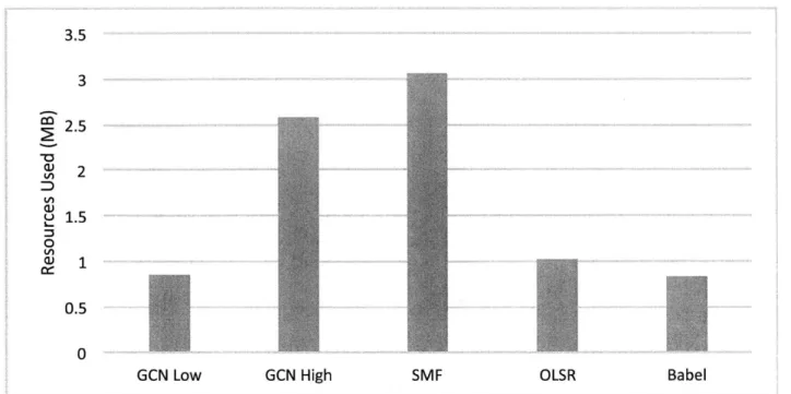
Figure 7.3: Network resources used, One-to-Many

data, and GCN with high resiliency (higher redundancy) transmits about 4 MB. SMF uses over 5 MB, more than GCN on high resiliency and much more than GCN on low resiliency. All three protocols delivered 100% of the traffic in this scenario, so GCN with low resiliency is optimal for this topology.

As we scale to 60 and then 90 nodes we see that GCN on low resiliency's data usage does not change. GCN on higher resiliency does use more data as density increases. When there were only 30 nodes in the network GCN on high resiliency often could not find as many relays as it wanted. If a node only has three neighbors, no matter how high the resiliency parameter that node can have at most three neighboring relays. Increasing the topology to 90 nodes allows GCN's high resiliency to find the relays it wants, so it sends more traffic through the network.

(45)

200

150

100

0 30 node

E

60 node

50

E

90 node

50

(1)

0 GCN

GCN

SMF

OLSR

Babel

Low

High

Figure 7.4: Network resources used, Many-to-One

Many-to-One

Figure 7.4 shows the amount of resources used in bytes in the Many-to-One traffic pattern. This pattern requires many nodes to send data back to a single node, so there are far more flows in the network than there were in the one-to-many pattern. Due to the increased number of packets, GCN, SMF, and OLSR are less efficient. At any network density SMF uses more resources than any other protocol. Its high delivery rate clearly comes at a cost to the network. Networks with low data rates, like military tactical networks, would be unable to handle the sheer volume of data transmitted over-the-air.

Of course, all of the protocols are going to use more data as the number of nodes increases.

Since one quarter of the nodes in the network are designated as sources, the 90 node test has far more sources than the 30 node network does. However, GCN scales into the more intensive traffic pattern significantly better than SMF does. GCN's data usage increases

nearly linearly: GCN uses 10MB, 25MB, and 40MB at 30, 60, and 90 nodes respectively. SMF's usage skyrockets from 30MB to 100MB to 190MB.

(46)

For the 90 node topology GCN with high resiliency uses 40MB, and GCN with low resiliency uses 20MB. OLSR and Babel transmit 25 and 50 MB, respectively. GCN uses a similar amount of resources as Babel and OLSR in the many-to-one scenario, but it achieves a much better delivery percentage in doing so. Recall from Figure 7.2 OLSR and Babel struggled to deliver 30% of the data, while either GCN resiliency delivered 70%. OLSR and Babel would be inappropriate for a military network because the links between tactical devices are very lossy. GCN, however, is more likely to deliver data and could tolerate the lossy links.

7.2 In-depth Results

In this section we will look at each individual test run and expand upon the packet delivery rate and resources used. We will look at a series of tests that examine network size, network density, packet rate, and topology. We begin with 9 node experiments in Clique and Chain topologies, then we move on to 30, 60, and 90 node tests in the office topology.

7.2.1 Clique

In the Clique topology every node can hear every other node. Due to WiFi limitations it is difficult to run Cliques of a large size, so we restrict ourselves to 9 devices.

The percentage of packets delivered in this experiment are presented in Figure 7.5. In a small clique we would expect all of the protocols to deliver a high percentage of the packets because there are no hops in the network. We see that GCN on high resiliency and SMF both deliver 100% of the packets, as expected.

GCN on low resiliency delivers 80% of the packets, more than OLSR and Babel but less than the higher resiliency GCN. In the clique there is only one source node, and very few of the nodes in the network are group nodes. At low resiliency very few of the non-group nodes

Deployment of a next generation networking protocol