Assessing membership projection errors in star forming regions

(1)

HAL Id: hal-03053271

https://hal.archives-ouvertes.fr/hal-03053271

Submitted on 10 Dec 2020

HAL is a multi-disciplinary open access

archive for the deposit and dissemination of

sci-entific research documents, whether they are

pub-lished or not. The documents may come from

teaching and research institutions in France or

abroad, or from public or private research centers.

L’archive ouverte pluridisciplinaire HAL, est

destinée au dépôt et à la diffusion de documents

scientifiques de niveau recherche, publiés ou non,

émanant des établissements d’enseignement et de

recherche français ou étrangers, des laboratoires

publics ou privés.

Assessing membership projection errors in star forming

regions

T. Roland, C. M. Boily, L. Cambrésy

To cite this version:

T. Roland, C. M. Boily, L. Cambrésy. Assessing membership projection errors in star forming

re-gions. Astronomy and Astrophysics - A&A, EDP Sciences, 2020, 644, pp.A141.

�10.1051/0004-6361/202039118�. �hal-03053271�

(2)

A&A 644, A141 (2020) https://doi.org/10.1051/0004-6361/202039118 c T. Roland et al. 2020

Astronomy

&

Astrophysics

Assessing membership projection errors in star forming regions

T. Roland, C. M. Boily, and L. Cambrésy

Université de Strasbourg, CNRS, Observatoire Astronomique de Strasbourg, UMR 7550, 67000 Strasbourg, France e-mail: timothe.roland@astro.unistra.fr

Received 6 August 2020/ Accepted 19 October 2020

ABSTRACT

Context.Young stellar clusters harbour complex spatial structures emerging from the star formation process. Identifying stellar over-densities is a key step in better constraining how these structures are formed. The high accuracy of distances derived from Gaia DR2 parallaxes still do not allow us to locate individual stars within clusters of ≈1 pc in size with certainty.

Aims.In this work, we explore how such uncertainty on distance estimates can lead to the misidentification of membership of sub-clusters selected by the minimum spanning tree (MST) algorithm. Our goal is to assess how this impacts their estimated properties.

Methods.Using N-body simulations, we build gravity-driven fragmentation models that self-consistently reproduce the early stellar configurations of a star forming region. Stellar groups are then identified both in two and three dimensions by the MST algorithm, representing respectively an inaccurate and an ideal identification. We compare the properties derived for these resulting groups in order to assess the systematic bias introduced by projection and incompleteness.

Results.We show that in such fragmented configurations, the dynamical mass of groups identified in projection is systematically underestimated compared to those of groups identified in 3D. This systematic error is statistically of 50% for more than half of the groups and reaches 100% in a quarter of them. Adding incompleteness further increases this bias.

Conclusions.These results challenge our ability to accurately identify sub-clusters in most nearby star forming regions where distance estimate uncertainties are comparable to the size of the region. New clump-finding methods need to tackle this issue in order to better define the dynamical state of these substructures.

Key words. methods: statistical – stars: formation – stars: kinematics and dynamics – open clusters and associations: general

1. Introduction

Young stars are predominantly observed in the dense parts of spiral arms of disc galaxies. After a decade of Herschel obser-vations, it is now established that these star forming regions exhibit highly sub-structured configurations due to fragmen-tation of the gas in extended filaments (André et al. 2010;

Pokhrel et al. 2018). The latest interferometric facilities (e.g., ALMA, NOEMA) allow to study filaments and primordial cores at sub-parsec scales (see e.g., Hacar et al. 2017, 2018;

André et al. 2019;Montillaud et al. 2019), bringing to light the very last stage of the transformation of gas into stars. Stars emerge from this network in groups of varying size and mor-phology. However, their kinematics is at odds with that of their natal gas (Foster et al. 2015). Moreover, their dynamical state is poorly constrained (Kuhn et al. 2019) and their fate uncertain.

The new era of precise astrometry opened by Gaia DR2 enables exploration of the spatial and kinematic proper-ties of a huge number of young stellar systems (see e.g.,

Kounkel & Covey 2019; Cantat-Gaudin et al. 2019 for the

newest catalogs of Gaia-discovered stellar clusters). In the solar neighbourhood, the 3D structure of local star forming clouds is within our reach. Großschedl et al.(2018) measured the extended 3D structures of the Orion A tail, reporting an esti-mated total length of 90 pc, in significant disagreement with the projected size of 40 pc. Other large, extended structures have been identified outside the solar circle (e.g.,Alves et al. 2020). The astonishing accuracy of Gaia DR2 data peaks at MG ≈ 13,

but degrades steadily at fainter magnitudes. This leads to uncer-tainties in distance estimates affecting mostly low-luminosity or reddened stars. In young and embedded regions, identifying 3D

stellar structures at (sub-)parsec scales remains challenging. For instance, the selected sample ofKounkel et al.(2018) in Orion has a mean uncertainty on parallax measurements of ≈0.5 mas which corresponds to ≈8 pc at this distance (≈400 pc).

In this context, simulations are key to testing our under-standing of the processes acting in these fragmented regions. Recent computations of hydro-gravitational fragmentation and accretion, coupled with radiation-transfer physics, give promis-ing results in terms of for example the shape of the stellar mass function (e.g., Bate 2012), formation of proto-planetary discs (e.g., Hennebelle et al. 2016), and the role of stellar feedback (e.g.,Wall et al. 2020). Despite continued progress, the number of young stars produced in these high-resolution calculations is limited to a few hundred. Larger calculations remain challenging. Moreover, strong interactions between newly born stars occur in these simulations. Exploring the interplay between several of these systems is key to probing the formation of more massive clusters. Consequently, pure N-body modelling is still of great use to explore configurations with N > 1000 stars. This approach works well when gravity takes over magneto-thermal support and drives the fragmentation of the giant molecular cloud (GMC). This allows us to address specific topics such as primordial mass segregation (Pavlík et al. 2019) or the impact of gradual star for-mation (Farias et al. 2019). As massive clusters are also likely to form massive stars (Motte et al. 2018), N-body simulations are also suited to exploring the environment where they form.

There is a long-standing history of modelling stellar inter-actions with gravity alone. One major challenge of such work consists in generating realistic initial configurations. Different methods have been developed. One of the most straightforward is to follow snapshots of hydro-dynamical simulations and

Open Access article,published by EDP Sciences, under the terms of the Creative Commons Attribution License (https://creativecommons.org/licenses/by/4.0), which permits unrestricted use, distribution, and reproduction in any medium, provided the original work is properly cited.

(3)

the structures traced by sink particles (e.g., Moeckel & Bate

2010; Fujii & Portegies Zwart 2016). This approach is well

suited to exploring the long-term evolution of the original hydro-dynamical simulations, but is limited by the high compu-tational effort to model the full star formation process. An effi-cient alternative that can be used to reproduce the fragmented aspect of star forming complexes at lower cost was introduced by

Goodwin & Whitworth(2004), namely the box fractal method.

This technique can recreate spatial configurations of various observed clusters and allows the user to tune the different levels of substructures. However, the velocity field is not constrained by the history of formation of such structures which makes the dynamical state of the system somewhat ad hoc.

Another method providing a balance between computational cost and realistic configurations was proposed by Dorval et al.

(2016), which we refer to as gravity-driven fragmentation (GDF) models. This method is an efficient way to build fragmented ini-tial conditions self-consistently using only N-body modelling. It allows the user to explore a large number of fragmented config-urations and test our understanding of the dynamical processes in action (see alsoDorval et al. 2017).

In this paper, we specifically discuss morphological biases introduced when estimating properties of stellar over-densities in a fragmented cluster seen in projection. We used the GDF method to model a realistic distribution of stars in a young star cluster (Sect.2). Our methodology consists in identifying stellar groups of more than 50 members (also referred to as clumps), both in 3D and in projections (2D) and estimating their prop-erties (Sect. 3). We used the virial dynamical mass to com-pare groups identified by both methods and assess the deviation introduced by projection effect (Sect.4). Finally, we discuss the implications of our results in Sect.5and conclude in Sect.6.

2. Building realistic stellar distribution

2.1. Gravity-driven fragmentation modelling

We start our study using the GDF models described in

Dorval et al. (2016). We summarise here the motivations and

principles of such models.

The fragmentation of a continuous cold fluid bound by gravity will proceed from continued growth of a spectrum of perturbations. When dealing with stars, the point-mass nature and limited number of elements means that the potential is not smooth, and Poisson-seeded density fluctuations rapidly develop into dense substructures. The growth of small-scale modes will proceed on very short timescales, however large-scale modes will grow on the global gravitational timescale of ∼1/√Gρ0

which is the same as the free-fall timescale. To allow time for these fluctuations to develop well in the non-linear regime, one sets up a self-gravitating system uniformly populated by stars with an outward radial velocity field. The velocity flow is taken to be isotropic with respect to the barycentre of the system; its amplitude is such that the total binding energy remains negative, and so expansion stops after some time which we take to coin-cide with the formation timescale of massive stars.

This method allows us to simulate the two main physical processes driving the late stages of star formation: self-gravity, computed by a collisional N-body integrator; and adiabatic cool-ing of the system, driven by the expansion. We adopted such a modelling to reproduce the distribution of young stars in a filamentary network whose nodes are dense and asymmet-ric clumps. These clumps comprise between tens of stars and a few hundred, and are usually considered as the early

prod-ucts of the star formation process (Krumholz 2014). As the overall velocity field is self-consistently built, we are able to probe their dynamical state and interactions with their surround-ings. Furthermore, when using a mass spectrum, the most mas-sive stars attract the surrounding low-mass stars to themselves.

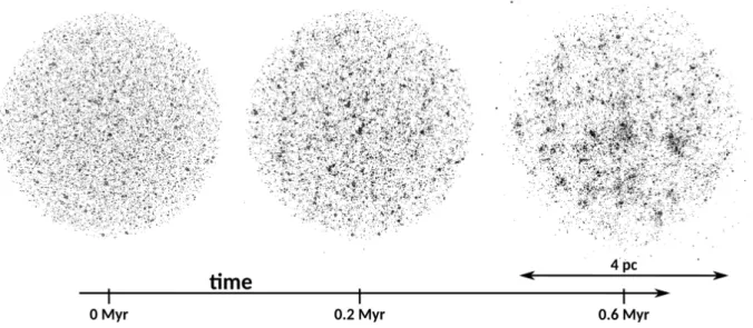
Dorval et al.(2016) showed that massive stars are the seeds for the growth of fragment modes. As a result, clumps are mass seg-regated at birth, retrieving a key feature of hydro-simulations (e.g.,Maschberger & Clarke 2011;Wall et al. 2019). They also harbour a top-heavy mass profile whose Salpeter index is compa-rable to the one found in young- and open clusters of the Milky Way (Bastian et al. 2010). Figure 1 shows the initial, interme-diate, and final steps for one of our models. More details and further examples are given inDorval et al.(2016,2017). 2.2. Simulation details

We based our study on a GDF model with N = 15 000 young stars following a canonical Kroupa-Chabrier initial mass func-tion (IMF; Kroupa et al. 2001; Chabrier 2003). We adopt the functional form ofMaschberger(2013) for efficiency. The initial velocity field is chosen so that the expansion stops roughly when the system is 4 pc in diameter, resulting in a mean density of ρ0≈ 150 Mpc−3.

These parameters probe the high-mass regime of young clus-ters close to the so-called young massive clusclus-ters (YMCs). They were chosen for several reasons.

– Firstly, these parameters allow us to accurately sample the IMF in the range 0.01−30 M. The high-mass end limit was

chosen in order to keep the mean mass of the system around ≈0.3 M. Indeed a specific draw of the IMF on 15 000 stars leads

to approximately ten stars more massive than 30 M1 and can

contribute as much as 10% of the mass budget of the overall region.

– Secondly, these allow us to reproduce a well-defined sam-ple of clumps of different memberships and densities. This is a direct consequence of including enough massive stars that act as the seeds of the formation of these clumps. In a theoretical “bottom up” scenario of star formation, where these clumps will subsequently merge together, such a system is a likely progeni-tor of a massive open cluster. This large range in densities (see Sect.2.3) allows us to probe different clump environments. How-ever, we note that such a crowded configuration can affect the level of contamination. In Sect. 5.2, we discuss a model with lower membership.

– Finally, with such parameters, the formation of the model lasts 0.55 Myr which matches the typical time for massive stars (>1 M) to reach the main sequence. This also corresponds to

the free-fall time of a GMC with density equal to ρ0,

t_ff = s

3π 32Gρ0

= 0.67 Myr. (1)

As most of the stars in a GMC are formed within a free-fall time (Grudi´c et al. 2018), this allows us to study the very early stages of the configuration of newly born stars. These structures have not yet been erased by two-body relaxation, and their dynamical state is a direct result of the fragmentation process.

We perform the computations with the AMUSE platform

(Portegies Zwart & McMillan 2018). We used the N-body code

1 _{The probability to draw a star more massive than 30 M}

is of the order of 10−4_{with N ∼ 10}4_.

(4)

T. Roland et al.: Assessing membership projection errors in star forming regions

Fig. 1.Gradual fragmentation of a GDF model in co-moving coordinates (physical length scale is only valid for the right panel). Left panel: initial step: stars are uniformly distributed and have radial velocities. Middle panel: growth of fluctuations in the expanding sphere. Right panel: point at which the system is fully fragmented and expansion stops.

ph4 which is a fourth-order Hermite scheme integrator cou-pled with the Multiple module to handle efficiently close interactions (Hut et al. 1995; McMillan & Hut 1996). The rel-ative energy drift δE/E at each time-step is always lower than 10−6 _{except when close encounters cannot be resolved by the}

Multiple module, and can lead to an error up to 10−4. How-ever, these remain rare, which makes the total energy drift during the whole calculation of the order of 10−4. We do not explicitly include any binary population but they are able to form dynam-ically through the fragmentation process. However, the fraction of multiple stars remains below 5% and these do not influence our conclusions.

2.3. Sub-selection within the GDF model

Gravity-driven fragmentation models allow exploration of the structures built by the fragmentation process. In this study, we specifically target clumps that can be misidentified when only seen in projection. However, as we see in Fig.1, the spherical imprints of the initial conditions remain visible at the large scale. This overall geometry of the cluster can have an impact on the clumps that we identify in projection in the following section.

To this end, we implemented a method to extract a subsam-ple from the central parts of the system. This method is based on the HOP algorithm (Eisenstein & Hut 1998) which was initially designed to identify over-dense haloes in any particle-based sample. HOP assigns to each particle a local density estimate based on a list of nearest neighbours and groups them around density peaks. We adapted the HOP algorithm to select a sample representative of the complex structure of the GDF model span-ning a large-enough range in density. First, we tune the param-eters to select only particles with a local density above a given threshold. Several tests lead us to set the threshold value equal to ≈75 Mpc−3, or half of the median system density. We then

exclude groups that were close to the edge of the GDF sphere by retaining only those that included at least one member lying less than 1 pc from the centre of the model. This two-step procedure leads to the selection of a subsample of particles excluding about half of the stars.

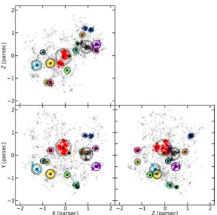
This new sample is the reference set for the rest of the study. Figure2shows three orthogonal views of the initial GDF

Fig. 2. Three orthogonal views of the GDF model. The full initial sample of stars is represented in grey shades and the sub-sample we extracted is shown in orange. Upper right panel: local density of the particles estimated by HOP stacked along the slice represented by the black rectangles on the three other views.

model (grey dots) and the selection of 7235 stars (orange dots). On the upper left panel, local densities of particles within a slice of the model (black rectangles) are plotted. This highlights that the selection retains all the main density peaks. Further-more, local densities span a large range, from ≈100 Mpc−3to

≈104_M pc−3.

3. Stellar groups

Stars are more likely to be formed in dense environments where the final collapse of gas is transformed into stars through an accretion process. The various stages of accretion2 means that

2 _{These are known as Class 0, I, II, III objects (see e.g.,}_{Andre et al.}

2000).

(5)

stars acquire their mass in a shared environment. Data from Herschelfor example have long indicated that the proximity of young stars gives rise to extended structures of varying morphol-ogy, all interconnected by a complex network of bridges and fil-aments. We are tasked with identifying the stars that belong to such a network.

3.1. Identification method

Several techniques have been developed to detect over-densities in observations of star forming regions. These include for example, the minimum spanning tree (MST) algorithm

(Gutermuth et al. 2009); the finite-mixture model technique

(Kuhn et al. 2014); DBSCAN (Joncour et al. 2018), and

HDB-SCAN (Kounkel et al. 2018). Despite their specific features, most of these techniques rely on star number density estimates projected on the sky3_{. This is mainly because of the few}

observ-ables available in such crowded regions, where extinction may be significant. By construction, these methods may miss the true underlying 3D structure of the objects under study.

We address the biases that arise from projection effects, focusing on the MST method. Its ability to detect over-dense structures of any shape makes it a powerful tool in studies of star forming regions. It has been widely used by both theorists (e.g.,

Maschberger et al. 2010) and observers (e.g., Kirk & Myers

2011; Beuret et al. 2017). MST statistics can also be used to

derive other properties of stellar clusters such as morphological aspects (Cartwright & Whitworth 2004) or a measure of mass segregation (Allison et al. 2009). Moreover, the MST method may be adapted to treat either 2D or 3D space distributions. Our setup described below was similarly implemented in both cases. This uniformity in the methodology is crucial in order to avoid introducing additional biases between 2D and 3D identifications. 3.2. Minimum spanning tree setup

We summarise the MST procedure briefly (see e.g.,

Gutermuth et al. 2009 for further details). A spanning tree

is a path linking all particles of a data set without forming closed loops. The MST is the spanning tree that minimises the total length of this path. We thus obtain a hierarchical set of edges that link every particle of the sample. To identify groups, we define a characteristic cut-off scale, dcut, such that all edges of

larger values will be removed from the MST set. This isolates star aggregates that are on average closer to each other. The choice of dcut is critical to our analysis: a large value will link

together stars that are very widely separated, revealing a few populous and sub-structured groups of stars ; on the other hand, a very small value will isolate binary and multiple stars, but will not reveal the hierarchical complex structure of the system as a whole. A natural way to pick a value for dcut is to count the

number S of subsets with a minimum membership, and vary dcut. When decreasing dcut from ≈R, the size of the system, it

is not too hard to see that S should rise from a value of 1 to a maximum value Smax and drop to ≈0 when dcut → 0. An

optimal value of dcutis found when maximising the number of

groups, S = Smax (see Dorval et al. 2016). However, this

iter-ative procedure can prove computationally costly. After some experimentation, we settled on a simple but efficient procedure based on the distribution of the MST edges. A characteristic

3 _{There are a few exceptions, for instance: HDBSCAN cited above or} the friends-of-friends algorithm (Huchra & Geller 1982) which both use spatial- and kinematic coordinates, but they are difficult to set up.

length is retrieved by adding one-half of a standard deviation to the mean value of MST edges. The cutting length dcutis set to

dcut= mean(EMST)+ std(EMST)/2, (2)

with EMSTbeing the set of MST edges. This way of fixing dcut

provides nearly optimal values without the iteration procedure. 3.3. Membership N

We fixed a minimum number of stars per stellar group, N, based on two arguments. The first is that we consider a system that is on the order of 1 Myr old, which is old enough for massive stars to have reached the main sequence, but not so old that the system as a whole has had time to settle into virial equilibrium. Hence, filaments and knots are transient features. On the other hand, we want the majority of these clumps to be as close as possi-ble to their state at formation: indeed, MST statistics cannot be used to gauge the equilibrium state of the substructures we aim to isolate. However, what is clear is that any substructure will evolve internally by phase mixing and kinetic-energy diffusion on a timescale of ∝1/√Gρ. We take as reference an average den-sity of 100γ Mpc−3, with γ being a dimensionless scalar. We

then compute a characteristic time tcr∼ 1.5/√γ × 106yr, which

we take as the dynamical timescale for motion driven by grav-ity. When a number N of stars are bound together, their repeated interactions lead to diffusion of kinetic energy on a timescale trel

given by (e.g.,Meylan & Heggie 1997):

trel' 0.138

Rh

2Rv

!32 _N

ln 0.4Ntcr. (3)

In the above relation, the ratio of half-mass radius Rhto virial

radius Rv = −GM/E (where E is the binding energy) is ≈1 for

self-gravitating configurations near equilibrium. We find trel> tcr

for N & 50, and furthermore trel > 1 Myr for γ ≤ 1. This tells

us that clumps with membership N of 50 or more should remain relatively close to their phase-space configuration at birth. Even so, the case for setting N= 50 becomes weaker in denser envi-ronments (γ 1), and we should increase N in proportion to √γ to avoid diffusion effects which drive dissolution. Clearly, a setup that will fit all situations is difficult to pin down; our ref-erence value= 50 also coincides with the membership of stellar associations seen in the low-density environments (Lada & Lada

2003; Gouliermis 2018). This value is also, in a loose sense,

motivated by observations. 3.4. Dynamical mass estimates

We apply the MST algorithm to the subsample defined in Sect.2.3twice: once using the full (3D) spatial coordinates, and once using only projected coordinates on the xy plane. Three orthogonal views of the resulting groups identified in 3D are plotted in Fig.3, and in 2D in Fig.4. This leads to the identifica-tion of approximately 16 groups in each case. However, the com-parison between these figures shows a different identification. In Fig.3, the main over-densities of the region are well retrieved in all projection panels; we refer to these as real groups, as they represent the ideal identification with the MST algorithm. By contrast, in Fig.4, group members appear well clumped only in the xy plane. On the other planes, they spread out over the whole area. These groups, henceforth projected groups, are biased in various ways: they can be real over-densities with some unre-lated contaminants; or, completely artificial structures whose

(6)

Fig. 3.Three orthogonal views of the sub-sample with real groups iden-tified by the MST in three dimensions. The black crosses show the loca-tion of the centre of mass of each group, and the circles show their 75% and 90% Lagrangian radii.

Fig. 4.Same as Fig.3but with projected groups identified by the MST in two dimensions along the xy plane (lower left panel). The projected Lagrangian radii are not tractable along the z-axis.

members are just aligned by chance in the line-of-sight. We emphasis the fact that this is different from the classical con-tamination by field stars, because all stars in our model are lying within the same star forming region of ≈4 parsec in diameter. Real and projected groups cannot be compared one to one. In order to compare both sets statistically, we quantify an observ-able property of these groups self-consistently.

With this in mind, we compute the dynamical mass which is a powerful tool to gauge the equilibrium state of a sys-tem (Portegies Zwart et al. 2010). It is also used to evaluate the dynamical state of young stellar systems and determine their fate (see e.g.,Kuhn et al. 2019). From the virial theorem, we define the dynamical mass Mdyn:

Mdyn= η ×

Reffσ2LOS

G , (4)

where Reff is the effective radius, and σLOS is the

line-of-sight velocity dispersion. The mass-to-light ratio, denoted η, depends on the phase-space configuration of the stellar system (Boily et al. 2005; Fleck et al. 2006). Hence all quantities that appear on the right-hand side of Eq. (4) are observables from projected data. This is crucial to compare Mdynfor real and

pro-jected groups in a self-consistent way.

As groups in our sample are asymmetric and not fully relaxed, we first determine the value of η empirically on real groups. This will constitute a value of reference to assess the dif-ference between real and projected groups (we discuss the value of η further in Sect.5.4).

To obtain an ensemble of ηs representative of each group, we estimate the dynamical mass of real groups from a large num-ber of different lines of sight, representing the possible viewing angles all over the sphere. To pick isotropic lines of sight, we chose the HEALPix tessellation (Górski et al. 2005) with the res-olution parameter Nside= 3, giving 192 different angles of view

separated by ≈14◦ each. Our procedure iterates over these lines of sight and re-computes the position and velocity of the whole sample to estimate the projected dynamical mass of real groups corresponding to each view. Finally, since the HEALPix tessel-lation is symmetric with respect to the centre of the sphere, each configuration is paired with its mirror image. As a result there are 192/2= 96 independent mass estimates for each real group. The effective radius in Eq. (4) is often replaced with the half-light radius in observational surveys of star clusters. The half-light radius matches the half-mass radius of ana-lytic King-Michie cluster models in equilibrium (Mengel et al.

2002;Wolf et al. 2010) which allows direct comparison between

observations and theory. However, this no longer holds true when the stellar clusters are mass-segregated (Gaburov & Gieles 2008). Moreover, the MST identifies asymmetric groups for which only one radius may not be representative of its size. Therefore, we explored different definitions of group radius cor-responding to the projected Lagrangian radii at 50%, 75%, 90%, and 100%.

Computing the line-of-sight velocity dispersion of groups identified by the MST is not trivial. Indeed groups are in close interaction with their environment and members nearer to the edge are likely to be affected by the surroundings. We address this issue by estimating four different velocity dispersions cor-responding to the stars lying within the four Lagrangian radii computed above. We also chose to compute the velocity disper-sion using the biweight scale estimator (Beers et al. 1990) which is more robust than the standard deviation when the distribution contains outliers.

4. Assessing projection bias

4.1. Real groups

We thus obtain four different sets containing 16 × 96 = 1536 dif-ferent estimates of the dynamical masses of real groups. These are plotted in Fig.5. The distributions of all these estimates for each group are summarised as box-plots, where the median is shown as an orange vertical tick mark; the 16th and 84th per-centiles by the box edges; and the extrema by the whiskers. The slope of the correlation between the dynamical and real mass in each panel matches the corresponding value of η for each radius. We compute this slope by a least-squares linear regression fit in each case. We see a clear correlation present at all radii, with a constant relative uncertainty of δη/η ≈ 0.12, an indication that the correlation still holds even when including stars at the group edges.

(7)

Fig. 5.Correlation between the true and dynamical mass of real groups. Each panel shows different chosen radii for the dynamical mass estimate.

All possible values along different projecting angles for the same group are shown in a box-plot: the orange vertical tick marks represents the median of the distribution; the edge of the box, the 16th and 84th percentiles (such that 68% of the data are inside the box), and the horizontal bars correspond to the total width of the full distribution. The red lines are the least square fits on the data giving the values of η corresponding to each radius.

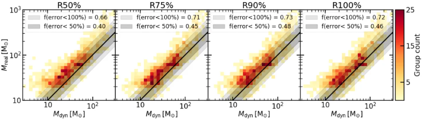
Fig. 6.Correlation between the true and dynamical masses of groups identified in projection represented as a 2D histogram. The black line shows the expectation constrained from real 3D groups (see Fig.5). Different shaded areas show the fraction of well-estimated group masses within an

error of 50% and 100%.

4.2. Projected groups

We focus now on the projected groups. We re-use the 96 view-ing angles of the whole region computed in Sect. 3.4to reach a similar number of mass estimates. As changing the line-of-sight will result in a different identification of projected groups, we re-compute the MST in each projection. Small vari-ations in the number of groups identified in each projection lead to a different total number of projected groups of 1425. Their dynamical masses were estimated with the corresponding η fac-tors constrained above (Sect.3.4). The correlation with their real masses is plotted in Fig.6as a two-dimensional histogram. The black line shows the correlation derived from real groups. How-ever, all mass estimates are shifted to lower values, falling to the left of the one-to-one relation on the figure. This highlights the fact that the mass of a group is underestimated when viewed in projection, irrespective of its true mass. The trend is not different from one panel to another, confirming that it is not sensitive to the choice of the radius. Globally, the deficit is greater than 50% for more than half of the groups, reaching 100% for a quarter of them. We attribute this systematic error to the misidentifica-tion of clumps due to projecmisidentifica-tion effects. As all radii are affected, the centre and the outskirts of projected groups are similarly impacted.

To further investigate the reason for this deviation, we also compared radii and velocity dispersions of real and projected groups with similar masses. We divided both sets into three bins

in terms of mass: [15; 35] M, [35; 100] Mand [100; 300] M.

The results corresponding to the 90% Lagrangian radii are plotted in Fig.7, but other radii give similar trends. We take a statistical approach to explore differences between real and pro-jected groups. The distributions within each mass bin are rep-resented by box plots of different colours: black for real groups and blue for projected groups. We recover on the left panel the systematic error in dynamical mass between real and projected groups (previously seen on Fig.6). The two other panels show the respective distributions of radii and velocity dispersions used to compute the dynamical mass. The properties of projected groups in a given mass bin are statistically lower than those of real groups. Moreover, the trend is more pronounced for the most massive groups. For the less massive groups, their Lagrangian radii are globally comparable whereas their velocity dispersions are systematically about 20% lower. We note here that this is not the case when choosing only the stars lying in the 50% or 75% Lagrangian radii where Poissonian fluctuations can increase the difference up to ≈30%. For groups more massive than 100 M,

both radii and velocity dispersions are equally shifted by about 30%, independently of the chosen radius.

In summary, projection effects lead to significant underes-timation of both the size and velocity dispersion of projected groups. Only the radii of the less massive groups are nearly not affected. Some may find it surprising that the velocity disper-sion is lowered in projected groups where some stars are not part of any clumps. However, we must bear in mind that these

(8)

Fig. 7.Comparison between projected and real group properties for three mass bins: [15; 35] M, [35; 100] Mand [100; 300] M(dashed lines). Distributions of each estimate are represented as black box plots for real groups and blue ones for projected groups. The relative error on the median for each distribution is annotated in red. In each box plot, the vertical middle tick represents the median of the distribution, the edges show the 16th and 84th percentiles, and the whiskers correspond to the full extension of the distribution. The estimates plotted correspond to the 90% Lagrangian radii but other radii give similar trends. The height of the boxes is proportional to the number of groups inside each mass bin. The 2D histogram of Fig.6is over-plotted on the panel of the dynamical mass estimate.

Fig. 8.Comparison of the dynamical mass estimated on projected groups with different levels of incompleteness. The three panels correspond to

the different real mass bins chosen in Fig.7. The black histogram is the reference set of real groups and the blue histogram is the set of complete projected groups. The histograms in green, orange and red represents projected groups that are only complete down to 0.3 M, 0.5 Mand 1 M respectively. The figure shows the results using the 90% Lagrangian radii.

stars are in the same region, and therefore they are likely to have a velocity close to the mean value (of ≈0 km s−1in our case, see Sect.5.1), which is the reason for the lower velocity dispersion in projected groups.

4.3. Incompleteness

Projection effects are always present in astronomical observa-tions where spherical symmetry is a valid ansatz. This eases comparison with theoretical models. However, this assumption is not justified for young systems. We indeed show that a lack of precise information in the line of sight can introduce systematic biases in the clump properties.

Another common bias when studying young stellar systems arises from incompleteness of the target populations. This also affects particularly star forming regions where extinction can be significant. We may estimate the importance of the complete-ness of the sample in comparison with that of the morphological projection biases that we have been discussing so far. At first order, the faintest sources are also the least massive ones, and so we apply different mass cuts to the set of projected groups (at 0.3 M, 0.5 M and 1 M). Again, we estimated the properties

of the resulting groups on the different lines of sight. Figure8

shows the resulting dynamical mass distribution within the three mass bins defined earlier in Fig.7. Distributions of real groups and complete projected groups from Fig.7 are also plotted for comparison. We observe that the distribution of dynamical mass estimates is progressively shifted to smaller values when incom-pleteness increases. This trend is expected, because the more massive stars selected are segregated in space over a smaller volume (Dorval et al. 2016), while their velocity dispersion will also be lower due to star–star interactions. As incompleteness of the sample will always increase the scatter owing to lower num-ber statistics, dynamical mass distributions of incomplete groups show greater dispersion.

This analysis is just the first step in a longer process, as we know that the problem of incompleteness is complex. Detection limits of observations is wavelength dependant and extinction is never constant inside the same star forming regions. Indeed, dust clouds also harbour filamentary structures in interaction with newly born stars and dramatically modify the aspects of these clusters. Other important additions are the stellar photom-etry and interstellar reddening, two quantities affecting the sam-pling of stars with opposite results. Indeed, the most massive

(9)

stars are the brightest but are also likely to be the most embed-ded (Motte et al. 2018). A self-consistent simulation including hydrodynamics would be needed to more accurately explore these aspects.

5. Discussion

5.1. Decontamination

We recall that the stars contaminating the set of projected groups are stars from the same region, separated only by a few par-secs and sharing the same global dynamical state. Therefore, it can be difficult to distinguish between contaminants and group members based on their kinematics alone. We ask if Gaia DR2 proper motions can separate two groups seen in projection using their individual proper motions. If we use a reference distance to Orion of 400 pc (Kounkel et al. 2018), the highest accuracy of Gaia DR2 proper motions is 0.1 km s−1 _{at M}

G = 13 but only

reaches 1 km s−1 at MG = 18. As Gaia EDR3 will improve

this value by a factor of two, we can expect to distinguish between two groups separated by a systematic motion of more than 0.5 km s−1_.

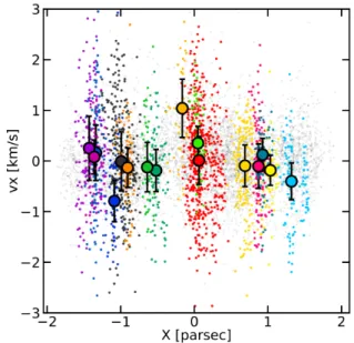
Figure9shows a one-dimensional position–velocity plot of stars in real (3D) groups. Each point is colour-coded as in Fig.3. Field stars are shown in light grey. The filled circles are the mean values for each group and the error-bars represent the standard deviation, which is an estimate of the typical internal motion of the clumps. An indication of the relative motions between these groups is given by the standard deviation of these mean values, which is ≈0.4 km s−1. This is of the same order as the internal motion, which is ≈0.5 km s−1. We conclude that the majority of real groups cannot be differentiated. We find only one instance where two out of sixteen groups are separated by ≈2 km s−1 which is within the Gaia detection limit. This is by construc-tion a feature brought by our GDF method, because we did not introduce large-scale motion in our fragmentation method. Such large-scale modes can be included in a future study.

5.2. Varying the total number of stars in the region

Although the reference set of 15 000 stars we previously studied allows us to explore clumps of different membership and den-sity, the large projected density of ≈500 stars pc−2can have an impact on the level of contamination of these clumps. Moreover, such clumpy configurations are not always seen in star form-ing regions. However, it is clear that none of the star formform-ing regions are perfectly isolated (Kuhn et al. 2014). The local envi-ronment of a particular region, even if it is not as structured as in our reference model, can still introduce some biases when inferring its properties. To probe such conditions, we built a GDF model with only 1000 stars and repeated the analysis. The sub-selection method with the HOP algorithm (Sect.2.3) extracts a sample of 765 stars for a surface density of 50 stars pc−2. This new model is, as expected, less structured: only one major over-density developed at the centre of the region (see upper panel of Fig.10). We therefore focus on this single clump detected by the MST. However, some structures exist in its environment that may contaminate it when seen in projection. We performed the esti-mation of the dynamical mass of this single group as in Sect.3.4. We used the values of η constrained previously in Sect.3.4. We also identify groups in projection for the same 96 lines of sight4

4 _{We note here that the MST identifies sometimes more than one group} in projection. In such cases, we only retain the most massive one.

Fig. 9.Position–velocity plot of stars in the sample. Stars that do not belong to any group are coloured in light grey whereas those in real 3D groups match the colours used in Fig.3. The filled circles are the mean values for each group and the error-bars represent the standard deviation.

and estimate their dynamical mass too. Finally we compare the distribution of both estimations. The distributions corresponding to the 75% Lagrangian radii can be seen in the bottom panel of Fig.10. Other radii show similar behaviours. The true mass of the group is marked as the red line for reference. The results are similar to those shown in Fig. 8: the dynamical mass of the projected group is systematically lower than that of the real group. Therefore, even the smaller number of sub-structures in this model can still lead to inaccurate estimation of clump prop-erties. Second, although the value of η was not calibrated on this model, the dynamical mass is well retrieved in 3D. Our over-all conclusions are therefore not sensitive to the precise surface density at least from 50 stars pc−2to 500 stars pc−2.

5.3. Clump-finding algorithm

Our study specifically aims to assess the bias introduced by pro-jection effects within a star forming region. We show that project effects systematically lower the spatial and kinematic properties of clumps. However, the amplitude of this shift is difficult to quantify. The variation that we estimate to range from 10 to 30% is due to the intrinsic nature of projection bias, which depends on the shape and orientation of a particular region. It is also linked to the method we choose.

However, most clump-finding algorithms also use projected spatial coordinates. For instanceJoncour et al.(2018) proposed a method to calibrate the DBSCAN algorithm using a sta-tistical approach. The DBSCAN is a close alternative to the MST. These latter authors exploit the nearest-neighbour statis-tics of a 2D Poissonian distribution to compute the parameters of the DBSCAN. This allows them to select only projected over-densities at three-sigma level over random expectation. Never-theless, this method is most suitable for small-scale structures of approximately ten members, where contamination in the line of sight is weak. For bigger clumps, like those that we identi-fied in the present study, projection effects are more significant. Therefore, we may expect that such a method will lead to similar results to the MST approach adopted here.

(10)

Fig. 10.Upper panel: sub-sample extracted from a GDF model of 1000 stars with the method of Sect.2.3. Only one major group is identified in 3D by the MST (red dots). Lower panel: distributions of the dynamical mass estimated on different projections of the main group identified by the MST in 3D (black line) and in projection (blue line). The true mass is marked as the vertical red line.

A step forward would be to build a set of GDF models repro-ducing configurations of a wide range in density, and train a machine-learning algorithm on this sample to bridge the 3D identifications to 2D projections with a significance estimator, similarly to what was developed by Joncour et al. (2018) for DBSCAN. We show here that all groups show comparable pro-jection biases, with a trend of increasing amplitude with group mass. This suggests that a data set of models with reasonably small groups –of up to 1000 stars– should still yield useful statis-tics while remaining manageable in terms of volume. Further work in that direction is underway.

5.4. The mass-to-light ratioη

A secondary result emerging from this study is the value of the mass-to-light ratio η linking the true and dynamical masses of real groups (see Sect.3.4). The value η ∼ 10 is often chosen to match a wide range of spherical King-Mitchie models (Spitzer 1987;Mengel et al. 2002). However,Fleck et al.(2006) already showed that η varies tremendously through the lifetime of a clus-ter, mostly as a result of mass segregation.

The value η ' 10 is about a factor three greater than our evaluation of ≈3.4 for real groups. Previous works (see e.g.,

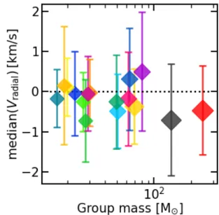
Fig. 11.Median of the radial velocity of stars in real groups with respect to their centre of mass. The colours are chosen to match those in Fig.3.

Portegies Zwart et al. 2010; Parker & Wright 2016) predicted that low values of η could be a signature property of young systems, one related to their state of equilibrium. As nothing suggests that real groups are in virial equilibrium, such a low value of η could be an indication of expansion. We rule out this explanation by computing the radial velocities of stars in real groups from their respective centres of mass. The median for each group is plotted in Fig.11. It shows that real groups are in a quasi-steady state, with vr ' 0 km s−1. This is perhaps

surpris-ing, because they are in close interaction with their environment, for instance through the tidal field of neighbouring groups and fly-by stars. However, it must be borne in mind that these con-figurations are a snapshot taken after only t ' 0.5 Myr. The age of the system is of the same order as the dynamical crossing time for groups, when little internal kinetic energy diffusion has had time to drive expansion.

Precise determination of η should help observers to put fur-ther observational constraints on the dynamical state of sub-clusters in star forming regions. For instanceKuhn et al.(2019) recently computed the virial-expected velocity dispersion of 19 young clusters. A lack of constraints on the value of η has pre-vented confirmation of the equilibrium dynamical state of these systems. Assuming a value of 10 leadKuhn et al.(2019) to con-clude that all of these clusters were unbound, although their Gaia proper motions did not show clear signs of expansion. Using a reduced value of 5, closer to our evaluation, would recon-cile these contradictory results. We stress that the systems that we have analysed, which are of linear scale '0.5 pc or less, are small compared to those ofKuhn et al.(2019). To make a more meaningful comparison with their survey would require that we develop models of a full-size '100 pc region, with disc-shearing and the vertical disc structure of the Milky Way added to the GDF modelling of Sect.2. We hope to report on these aspects in a future contribution.

6. Conclusions

In the present study, we use GDF models to self-consistently reproduce a fragmented distribution of stars to assess the sys-tematic bias introduced by an imprecise identification of stellar clumps in projection compared to an ideal one in 3D. To this end,

(11)

we performed a statistical comparison between the properties of stellar over-densities (of membership Nstars > 50) identified in

3D and in projection by a generic MST algorithm within a sin-gle star forming region of ≈4 pc in width5_{. Our main results can}

be summarised as follows:

1. We highlight that the dynamical mass of clumps identified in projection is systematically underestimated compared to the ideal 3D identification. This systematic error is greater than 50% in about half of the cases and can reach up to 100% in a quarter of them. This is due to the incorrect selection of the clump-finding algorithm when dealing only with projected coordinates in such fragmented regions.

2. This projection bias impacts both radius and velocity dis-persion estimates of projected groups. Eliminating potential outliers at the edges of the groups identified by the MST did not lead to any improvements.

3. We notice a trend ranging from the properties of less massive (M < 100 M) groups, which are less affected or even not

at all, to those of the most massive groups (M > 100 M),

which are more systematically affected. For these latter, radii and velocity dispersions are statistically 30% lower.

4. As the projection effect is not the only bias in star forming regions, we also considered simple prescriptions to account for incompleteness in the observations. We show that sam-ple incomsam-pleteness increases the systematic error. However, its impact is of a different nature and can be seen as a blur-ring effect. For example, the most massive groups are almost unaffected since they still contain a sufficient number of mas-sive members for them to be characterised.

5. We conclude that projection effects are the main limitation in estimating properties of clumps identified within a sin-gle fragmented region with no or insufficiently accurate dis-tance estimates. For most nearby star forming regions, the best Gaia parallaxes have uncertainties of a few percent. For these distant regions, that is, at more than 100 pc, this pre-vents any clump-finding algorithm from properly defining clumps of less than a few parsecs in size. Accurate identifica-tion of such clumps is a key challenge in better constraining the processes of star formation. This also has major impli-cations for predicting the future of these young systems in bound clusters or unbound associations.

6. We also show that GDF models offer an efficient method to initialise N-body simulations of young clusters. With this method, we are able to explore the structures built by gravity alone in more detail in order to better understand the role of gravity compared to the many processes at play in star form-ing regions.

Acknowledgements. We thank the referee for the constructive remarks which led to improve the quality of the paper. Timothé Roland also acknowledges Paolo Bianchini, Caroline Bot, Joe Lewis and Jonathan Chardin for their helpful comments and suggestions. This work has used the AMUSE framework (https://github.com/amusecode/amuse) (Portegies Zwart & McMillan 2018;Portegies Zwart et al. 2009,2013;Pelupessy et al. 2013) and the Python programming language with the following packages: matplotlib (Hunter 2007), NumPy (Harris et al. 2020), SciPy (Virtanen et al. 2020) and Astropy (Astropy Collaboration 2013,2018).

References

Allison, R. J., Goodwin, S. P., Parker, R. J., et al. 2009,MNRAS, 395, 1449

Alves, J., Zucker, C., Goodman, A. A., et al. 2020,Nature, 578, 237

5 _{We recall that we did not take into account any additional foreground} or background contamination besides the one introduced by the region itself.

André, P., Men’shchikov, A., Bontemps, S., et al. 2010,A&A, 518, L102

André, P., Arzoumanian, D., Könyves, V., Shimajiri, Y., & Palmeirim, P. 2019,

A&A, 629, L4

Andre, P., Ward-Thompson, D., & Barsony, M. 2000, inProtostars and Planets IV, eds. V. Mannings, A. P. Boss, & S. S. Russell, 59

Astropy Collaboration (Robitaille, T. P., et al.) 2013,A&A, 558, A33

Astropy Collaboration (Price-Whelan, A. M., et al.) 2018,AJ, 156, 123

Bastian, N., Covey, K. R., & Meyer, M. R. 2010,ARA&A, 48, 339

Bate, M. R. 2012,MNRAS, 419, 3115

Beers, T. C., Flynn, K., & Gebhardt, K. 1990,AJ, 100, 32

Beuret, M., Billot, N., Cambrésy, L., et al. 2017,A&A, 597, A114

Boily, C. M., Lançon, A., Deiters, S., & Heggie, D. C. 2005,ApJ, 620, L27

Cantat-Gaudin, T., Jordi, C., Wright, N. J., et al. 2019,A&A, 626, A17

Cartwright, A., & Whitworth, A. P. 2004,MNRAS, 348, 589

Chabrier, G. 2003,PASP, 115, 763

Dorval, J., Boily, C. M., Moraux, E., Maschberger, T., & Becker, C. 2016,

MNRAS, 459, 1213

Dorval, J., Boily, C. M., Moraux, E., & Roos, O. 2017,MNRAS, 465, 2198

Eisenstein, D. J., & Hut, P. 1998,ApJ, 498, 137

Farias, J. P., Tan, J. C., & Chatterjee, S. 2019,MNRAS, 483, 4999

Fleck, J. J., Boily, C. M., Lançon, A., & Deiters, S. 2006,MNRAS, 369, 1392

Foster, J. B., Cottaar, M., Covey, K. R., et al. 2015,ApJ, 799, 136

Fujii, M. S., & Portegies Zwart, S. 2016,ApJ, 817, 4

Gaburov, E., & Gieles, M. 2008,MNRAS, 391, 190

Goodwin, S. P., & Whitworth, A. P. 2004,A&A, 413, 929

Górski, K. M., Hivon, E., Banday, A. J., et al. 2005,ApJ, 622, 759

Gouliermis, D. A. 2018,PASP, 130, 072001

Großschedl, J. E., Alves, J., Meingast, S., et al. 2018,A&A, 619, A106

Grudi´c, M. Y., Hopkins, P. F., Faucher-Giguère, C.-A., et al. 2018,MNRAS, 475, 3511

Gutermuth, R. A., Megeath, S. T., Myers, P. C., et al. 2009,ApJS, 184, 18

Hacar, A., Tafalla, M., & Alves, J. 2017,A&A, 606, A123

Hacar, A., Tafalla, M., Forbrich, J., et al. 2018,A&A, 610, A77

Harris, C. R., Millman, K. J., van der Walt, S. J., et al. 2020,Nature, 585, 357

Hennebelle, P., Commerçon, B., Chabrier, G., & Marchand, P. 2016,ApJ, 830, L8

Huchra, J. P., & Geller, M. J. 1982,ApJ, 257, 423

Hunter, J. D. 2007,Comput. Sci. Eng., 9, 90

Hut, P., Makino, J., & McMillan, S. 1995,ApJ, 443, L93

Joncour, I., Duchêne, G., Moraux, E., & Motte, F. 2018,A&A, 620, A27

Kirk, H., & Myers, P. C. 2011,ApJ, 727, 64

Kounkel, M., & Covey, K. 2019,AJ, 158, 122

Kounkel, M., Covey, K., Suárez, G., et al. 2018,AJ, 156, 84

Kroupa, P., Aarseth, S., & Hurley, J. 2001,MNRAS, 321, 699

Krumholz, M. R. 2014,Phys. Rep., 539, 49

Kuhn, M. A., Feigelson, E. D., Getman, K. V., et al. 2014,ApJ, 787, 107

Kuhn, M. A., Hillenbrand, L. A., Sills, A., Feigelson, E. D., & Getman, K. V. 2019,ApJ, 870, 32

Lada, C. J., & Lada, E. A. 2003,ARA&A, 41, 57

Maschberger, T. 2013,MNRAS, 429, 1725

Maschberger, T., & Clarke, C. J. 2011,MNRAS, 416, 541

Maschberger, T., Clarke, C. J., Bonnell, I. A., & Kroupa, P. 2010,MNRAS, 404, 1061

McMillan, S. L. W., & Hut, P. 1996,ApJ, 467, 348

Mengel, S., Lehnert, M. D., Thatte, N., & Genzel, R. 2002,A&A, 383, 137

Meylan, G., & Heggie, D. C. 1997,A&ARv, 8, 1

Moeckel, N., & Bate, M. R. 2010,MNRAS, 404, 721

Montillaud, J., Juvela, M., Vastel, C., et al. 2019,A&A, 631, A3

Motte, F., Bontemps, S., & Louvet, F. 2018,ARA&A, 56, 41

Parker, R. J., & Wright, N. J. 2016,MNRAS, 457, 3430

Pavlík, V., Kroupa, P., & Šubr, L. 2019,A&A, 626, A79

Pelupessy, F. I., van Elteren, A., de Vries, N., et al. 2013, A&A, 557, A84

Pokhrel, R., Myers, P. C., Dunham, M. M., et al. 2018,ApJ, 853, 5

Portegies Zwart, S., & McMillan, S. 2018,Astrophysical Recipes: The Art of AMUSE, 2514-3433(AAS IOP Astronomy Publishing)

Portegies Zwart, S., McMillan, S., Harfst, S., et al. 2009,New Astron., 14, 369

Portegies Zwart, S. F., McMillan, S. L. W., & Gieles, M. 2010,ARA&A, 48, 431

Portegies Zwart, S., McMillan, S. L. W., van Elteren, E., Pelupessy, I., & de Vries, N. 2013,Comput. Phys. Commun., 184, 456

Spitzer, L. 1987, Dynamical Evolution of Globular Clusters (Princeton: Princeton University Press)

Virtanen, P., Gommers, R., Oliphant, T. E., et al. 2020,Nat. Meth., 17, 261

Wall, J. E., McMillan, S. L. W., Mac Low, M.-M., Klessen, R. S., & Portegies Zwart, S. 2019,ApJ, 887, 62

Wall, J. E., Mac Low, M. M., McMillan, S. L. W., et al. 2020, ApJ, accepted [arXiv:2003.09011]

Wolf, J., Martinez, G. D., Bullock, J. S., et al. 2010,MNRAS, 406, 1220