HAL Id: hal-02901192
https://hal.archives-ouvertes.fr/hal-02901192
Submitted on 16 Jul 2020
HAL is a multi-disciplinary open access
archive for the deposit and dissemination of
sci-entific research documents, whether they are
pub-lished or not. The documents may come from
teaching and research institutions in France or
abroad, or from public or private research centers.
L’archive ouverte pluridisciplinaire HAL, est
destinée au dépôt et à la diffusion de documents
scientifiques de niveau recherche, publiés ou non,
émanant des établissements d’enseignement et de
recherche français ou étrangers, des laboratoires
publics ou privés.
Distributed under a Creative Commons Attribution| 4.0 International License
Sets
Albert Cohen, Wolfgang Dahmen, Ronald Devore, James Nichols
To cite this version:
Albert Cohen, Wolfgang Dahmen, Ronald Devore, James Nichols. Reduced Basis Greedy Selection
Us-ing Random TrainUs-ing Sets. ESAIM: Mathematical ModellUs-ing and Numerical Analysis, EDP Sciences,
2020, 54 (5), pp.1509-1524. �10.1051/m2an/2020004�. �hal-02901192�
https://doi.org/10.1051/m2an/2020004 www.esaim-m2an.org
REDUCED BASIS GREEDY SELECTION USING RANDOM TRAINING SETS
Albert Cohen
1,*, Wolfgang Dahmen
2, Ronald DeVore
3and James Nichols
1Abstract. Reduced bases have been introduced for the approximation of parametrized PDEs in applications where many online queries are required. Their numerical efficiency for such problems has been theoretically confirmed in Binev et al. (SIAM J. Math. Anal. 43 (2011) 1457–1472) and DeVore et al. (Constructive Approximation 37 (2013) 455–466), where it is shown that the reduced basis space 𝑉𝑛 of dimension 𝑛, constructed by a certain greedy strategy, has approximation error
similar to that of the optimal space associated to the Kolmogorov 𝑛-width of the solution manifold. The greedy construction of the reduced basis space is performed in an offline stage which requires at each step a maximization of the current error over the parameter space. For the purpose of numerical computation, this maximization is performed over a finite training set obtained through a discretization of the parameter domain. To guarantee a final approximation error 𝜀 for the space generated by the greedy algorithm requires in principle that the snapshots associated to this training set constitute an approximation net for the solution manifold with accuracy of order 𝜀. Hence, the size of the training set is the 𝜀 covering number for ℳ and this covering number typically behaves like exp(𝐶𝜀−1/𝑠) for some 𝐶 > 0 when the solution manifold has 𝑛-width decay 𝑂(𝑛−𝑠). Thus, the shear size of the training set prohibits implementation of the algorithm when 𝜀 is small. The main result of this paper shows that, if one is willing to accept results which hold with high probability, rather than with certainty, then for a large class of relevant problems one may replace the fine discretization by a random training set of size polynomial in 𝜀−1. Our proof of this fact is established by using inverse inequalities for polynomials in high dimensions.
Mathematics Subject Classification. 62M45, 65D05, 68Q32, 65Y20, 68Q30, 35B30, 41A10, 41A25, 58D15, 65C99.
Received October 22, 2018. Accepted January 13, 2020.
1. Introduction
Complex systems are frequently described by parametrized PDEs that take the general form
𝒫(𝑢, 𝑦) = 0. (1.1)
Here 𝑦 = (𝑦𝑗)𝑗=1,...,𝑑 is a vector of parameters ranging over some domain 𝑌 ⊂ R𝑑 and 𝑢 = 𝑢(𝑦) is the
corresponding solution which is assumed to be uniquely defined in some Hilbert space 𝑉 for every 𝑦 ∈ 𝑌 .
Keywords and phrases. Reduced bases, performance bounds, random sampling, entropy numbers, Kolmogorov 𝑛-widths, sparse high-dimensional polynomial approximation.
1 Laboratoire Jacques-Louis Lions, Sorbonne Universit´e, Paris, France.
2 Department of Mathematics, University of South Carolina, Columbia, SC 29208, USA. 3 Department of Mathematics, Texas A&M University, College Station, TX 77840, USA. *Corresponding author: [email protected]
c
○ The authors. Published by EDP Sciences, SMAI 2020
This is an Open Access article distributed under the terms of theCreative Commons Attribution License(https://creativecommons.org/licenses/by/4.0), which permits unrestricted use, distribution, and reproduction in any medium, provided the original work is properly cited.
Throughout this paper, we denote by ‖ · ‖ and ⟨·, ·⟩ the norm and inner product of 𝑉 . In what follows, we assume that the parameters have been rescaled so that 𝑌 = [−1, 1]𝑑. Here 𝑑 is typically large and in some cases 𝑑 = ∞. We seek results that are immune to the size of 𝑑, i.e., are dimension independent.
Various reduced modeling approaches have been developed for the purpose of efficiently approximating the solution 𝑢(𝑦) in the context of applications where the solution map
𝑦 ↦→ 𝑢(𝑦), (1.2)
needs to be queried for a large number of parameter values 𝑦 ∈ 𝑌 . This need occurs for example in optimal design or inverse problems where such parameters need to be optimized. The strategy consists in first constructing in some offline stage a linear space 𝑉𝑛 of hopefully low dimension 𝑛, that provides a reduced map
𝑦 ↦→ 𝑢𝑛(𝑦) ∈ 𝑉𝑛, (1.3)
that approximates the solution map to the required target accuracy 𝜀 for all queries of 𝑢(𝑦). The reduced map is then implemented in the online stage with greatly reduced computational cost, typically polynomial in 𝑛.
As opposed to standard approximation spaces such as finite elements, the spaces 𝑉𝑛are specifically designed
to approximate the image of 𝑢, i.e., the elements in the parametrized family
ℳ := {𝑢(𝑦) : 𝑦 ∈ 𝑌 }, (1.4)
which is called the solution manifold. The optimal 𝑛-dimensional linear approximation space for this manifold is the one that achieves the minimum in the definition of the Kolmogorov 𝑛-width
𝑑𝑛= 𝑑𝑛(ℳ)𝑉 := inf dim(𝐸)=𝑛
sup
𝑢∈ℳ
‖𝑢 − 𝑃𝐸𝑢‖. (1.5)
This optimal space is computationally out of reach and the above quantity should be viewed as a benchmark for more practical methods. Here 𝑃𝐸 denotes again the 𝑉 -orthogonal projection onto 𝐸 for any subspace 𝐸 of
𝑉 .
One approach for constructing a reduced space 𝑉𝑛, which comes with substantial theoretical footing and will
be instrumental in our discussion, consists in proving that the solution map is analytic in the parameters 𝑦 and has a Taylor expansion
𝑢(𝑦) =∑︁ 𝜈∈ℱ 𝑡𝜈𝑦𝜈, (1.6) where 𝑦𝜈 :=∏︀𝑑 𝑗=1𝑦 𝜈𝑗
𝑗 and ℱ := {𝜈 ∈ N𝑑}. In the case of countably many parameters, ℱ is the set of finitely
supported sequences 𝜈 = (𝜈𝑗)𝑗≥1 with 𝜈𝑗∈ N. One then proves that the sequence (𝑡𝜈)𝜈∈ℱ of Taylor coefficients
has some decay property. Two prototypical examples of results on decay are given in [1,7] for the elliptic equation
−div(𝑎∇𝑢) = 𝑓, (1.7)
where the diffusion coefficient function has the parametrized form 𝑎 = 𝑎(𝑦) = 𝑎 +∑︁
𝑗≥1
𝑦𝑗𝜓𝑗, (1.8)
for some given functions 𝑎 and (𝜓𝑗)𝑗≥1. These results (see e.g. Thms. 1.1 and 1.2 in [1]) show that, under mild
decay or summability conditions on the functions 𝜓𝑗, one has that the sequence (‖𝑡𝜈‖𝑉)𝜈∈ℱ is in ℓ𝑝for certain
𝑝 < 1 with a bound on the ℓ𝑝quasi-norm. It then follows that for each 𝑛, there is a set Λ𝑛 ⊂ ℱ with #(Λ𝑛) = 𝑛
such that sup 𝑦∈𝑌 ‖𝑢(𝑦) − ∑︁ 𝜈∈Λ𝑛 𝑡𝜈𝑦𝜈‖ ≤ 𝐶𝑛−𝑟, 𝑟 := 1/𝑝 − 1. (1.9)
Similar results have been obtained for more general models of linear and nonlinear PDEs, see in particular [5,6], using orthogonal expansions into tensorized Legendre polynomials in place of Taylor series.
Therefore the space 𝑉𝑛 := span{𝑡𝜈 : 𝜈 ∈ Λ𝑛} has dimension 𝑛 with an a priori bound 𝐶𝑛−𝑟 on its
approximation error for all members of the solution manifold ℳ. One choice of Λ𝑛 giving (1.9) is the set of
indices corresponding to the 𝑛 largest ‖𝑡𝜈‖𝑉. Further analysis Cohen and Migliorat [8] shows that the same
convergence estimate can be obtained imposing in addition that the sets Λ𝑛are downward closed (or lower sets),
i.e. having the property
𝜈 ∈ Λ𝑛 and 𝜇 ≤ 𝜈 =⇒ 𝜇 ∈ Λ𝑛, (1.10)
where 𝜇 ≤ 𝜇 is to be understood componentwise. We stress that the rate of decay 𝑛−𝑟 in the bound (1.9) may be suboptimal compared to the actual rate of decay of the 𝑛-width 𝑑𝑛(ℳ).
The present paper is concerned with another prominent reduced modeling strategy known as the Reduced Basis Method (RBM). In this approach [10,11,14,15], particular snapshots
𝑢𝑘 = 𝑢(𝑦𝑘), 𝑘 = 1, 2, . . . , (1.11)
are selected in the solution manifold and the space 𝑉𝑛 is defined by
𝑉𝑛:= span{𝑢1, . . . , 𝑢𝑛}. (1.12)
A certain greedy procedure has been first proposed in [12] and analyzed in [3] for selecting these snapshots. It was shown in [2,9] that the approximation error
𝜎𝑛= 𝜎𝑛(ℳ)𝑉 := sup 𝑢∈ℳ
‖𝑢 − 𝑃𝑉𝑛𝑢‖, (1.13)
provided by the resulting spaces has the same rate of decay (polynomial or exponential) as that of 𝑑𝑛. In
this sense, the method leads to reduced models with optimal performance, in contrast to sparse polynomial expansions.
In its simplest (and idealized) form, the greedy procedure can be described as follows: at the initial step, one sets 𝑉0= {0}, and given that 𝑉𝑛 has been produced after 𝑛 steps, one selects the new snapshot by
𝑢𝑛+1:= argmax
𝑢∈ℳ
‖𝑢 − 𝑃𝑉𝑛𝑢‖. (1.14)
Each greedy step thus amounts to maximizing
𝑒𝑛(𝑦) := ‖𝑢(𝑦) − 𝑃𝑉𝑛𝑢(𝑦)‖ (1.15)
over the parameter domain 𝑌 . While in this precise form the scheme cannot be realized in practice an important modification of this greedy selection, known as the weak greedy algorithm, allows the selection to be done in a a practically feasible manner while retaining the same performance guarantees, see Section2below.
The optimization in the greedy algorithm is typically performed by replacing 𝑌 at each step by a discrete training set ˜𝑌 . In order to retain the performance guarantees of the greedy algorithm, this discretization should in principle be chosen fine enough so that the solution map 𝑦 ↦→ 𝑢(𝑦) is resolved up to the target accuracy 𝜀 > 0, that is, the discrete set
̃︁
ℳ = {𝑢(𝑦) : 𝑦 ∈ ˜𝑌 }, (1.16)
is an 𝜀-approximation net for ℳ.
Although performed in the offline stage, this discretization becomes computationally problematic when the parametric dimension 𝑑 is either large or infinite, due to the prohibitive size of this net as 𝜀 → 0. For example, in the typical case when the Kolmogorov width of ℳ decays like 𝑂(𝑛−𝑠) for some 𝑠 > 0, we can invoke Carl’s inequality [13] to obtain a sharp bound 𝑒𝑐𝜀−1/𝑠 for the cardinality of ˜ℳ and ˜𝑌 . This exponential growth
drastically limits the possibility of using 𝜀-approximation nets in practical applications when the number of involved parameters become large.
There is a preference toward the use of the greedy constructions over the Taylor expansion constructions because they guarantee error decay comparable to the decay of Kolmogorov widths while the Taylor polynomial constructions do not provide any such guarantee. Therefore, it is of interest to understand whether the apparent impediment of requiring such a fine discretization of the solution manifold can somehow be avoided or signifi-cantly mitigated. The main result of this paper is to prove that this is indeed the case provided that one is willing to accept error guarantees that hold with high probability rather than with certainty. Our main result shows that a target accuracy 𝜀 can generally be met with high probability by searching over a randomly discretized set ˜𝑌 whose size grows only polynomially in 𝜀−1 rather than exponentially, in contrast to 𝜀-approximation nets. The paper is organized as follows. In Section 2, we elaborate on the weak form of the greedy algorithm, which is used in numerical computation, and recall some known facts on its performance and complexity. In Section3, we use properties of downward closed polynomial approximation to show how a random sampling ˜𝑌 provides an approximate solution of the optimization problem engaged at each step of the greedy algorithm. In Section 4, we formulate our modification of the greedy algorithm based on such random selection and then analyze its performance. Finally, we illustrate in Section 5 the validity of the randomized approach by some numerical tests performed in parametric dimensions up to 𝑑 = 64 for which the size of 𝜀-approximation nets become computationally prohibitive.
2. Performance and complexity of reduced basis greedy algorithms
The greedy selection process described in the introduction is not practically feasible, due to at least three obstructions:
(1) Given a parameter value 𝑦, the snapshot 𝑢(𝑦), in particular, the generators of the reduced spaces cannot be exactly computed.
(2) For a given 𝑦 ∈ 𝑌 , the quantity 𝑒𝑛(𝑦) to be maximized cannot be exactly evaluated.
(3) The map 𝑦 ↦→ 𝑒𝑛(𝑦) is non-convex/non-concave and therefore difficult to maximize, even if it could be
exactly evaluated.
The first obstruction can be handled when a numerical solver is available for computing an approximation
𝑦 ↦→ 𝑢ℎ(𝑦), (2.1)
of 𝑢(𝑦) to any prescribed accuracy 𝜀ℎ> 0, that is, such that
sup
𝑦∈𝑌
‖𝑢(𝑦) − 𝑢ℎ(𝑦)‖ ≤ 𝜀ℎ. (2.2)
Here ℎ > 0 is a space discretization parameter: typically, 𝑢ℎ belongs to a finite element space 𝑉ℎ of meshsize ℎ
and (possibly very large) dimension 𝑛ℎ. The selected reduced basis functions are now given by 𝑢𝑖 = 𝑢ℎ(𝑦𝑖) ∈ 𝑉ℎ
and therefore the reduced basis space 𝑉𝑛is a subspace of 𝑉ℎ. Whenever the 𝑛-widths 𝑑𝑛decay much faster than
the approximation order provided by 𝑉ℎ the reduced space 𝑉𝑛 has typically much smaller dimension than 𝑉ℎ,
that is
𝑛 ≪ 𝑛ℎ. (2.3)
This yields substantial computational savings when using the reduced basis discretization in the online stage. Note that this numerical solver allows us in principle to also handle the second obstruction: we could now perform the greedy algorithm by maximizing at each step the quantity
which, in contrast to 𝑒𝑛(𝑦), can be exactly computed and satisfies
|𝑒𝑛(𝑦) − 𝑒𝑛,ℎ(𝑦)| ≤ 𝜀ℎ, 𝑦 ∈ 𝑌. (2.5)
In other words, the greedy algorithm is applied on the approximate solution manifold
ℳℎ:= {𝑢ℎ(𝑦) : 𝑦 ∈ 𝑌 }. (2.6)
While the quantity 𝑒𝑛,ℎ(𝑦) can in principle be computed exactly, the complexity of this computation depends,
at least in a linear manner, on the dimension 𝑛ℎ= dim(𝑉ℎ), which is typically much higher than 𝑛. Substantial
computational saving may still be obtained when maximizing instead an a posteriori estimator 𝑒𝑛,ℎ(𝑦) of this
quantity that satisfies
𝛼𝑒𝑛,ℎ(𝑦) ≤ 𝑒𝑛,ℎ(𝑦) ≤ 𝛽𝑒𝑛,ℎ(𝑦), 𝑦 ∈ 𝑌. (2.7)
The computation of 𝑒𝑛,ℎ(𝑦) for a given 𝑦 ∈ 𝑌 is based in particular on replacing the orthogonal projection
𝑃𝑉𝑛𝑢ℎ(𝑦) by a Galerkin projection. It, in turn, does not require the computation of 𝑢ℎ(𝑦) and entails a
compu-tational cost 𝑐(𝑛) depending on the small dimension 𝑛, typically in a polynomial way, rather than on the large dimension 𝑛ℎ. We refer to [6] for the derivation of a residual-based estimator 𝑒𝑛,ℎ(𝑦) having these properties in
the case of elliptic PDEs with affine parameter dependence.
Maximizing the a posteriori estimator 𝑒𝑛,ℎ(𝑦) amounts to applying to ℳℎa so called weak-greedy algorithm,
where 𝑢𝑛+1now satisfies
‖𝑢𝑛+1− 𝑃 𝑉𝑛𝑢
𝑛+1‖ ≥ 𝛾‖𝑢 − 𝑃
𝑉𝑛𝑢‖, 𝑢 ∈ ℳℎ, (2.8)
with parameter 𝛾 := 𝛼/𝛽 ∈ ]0, 1[.
For such an algorithm, it was proved in [2,9] that any polynomial or exponential rate of decay achieved by the Kolmogorov 𝑛-width 𝑑𝑛 is retained by the error performance 𝜎𝑛 for this algorithm. More precisely, the
following holds, for any compact set 𝒦 in a Hilbert space 𝑉 , see [6].
Theorem 2.1. Let 𝑑𝑛= 𝑑𝑛(𝒦)𝑉 be the 𝑛-widths of the solution manifold. Consider the weak greedy algorithm
with threshold parameter 𝛾. For any 𝐶0> 0 and 𝑠 > 0, we have
𝑑𝑛 ≤ 𝐶0(max{1, 𝑛})−𝑠, 𝑛 ≥ 0 =⇒ 𝜎𝑛≤ 𝐶𝑠𝛾−2(max{1, 𝑛})−𝑠, 𝑛 ≥ 0, (2.9)
where 𝐶𝑠:= 24𝑠+1𝐶0. For any 𝑐0, 𝐶0> 0 and 𝑠 > 0, we have
𝑑𝑛≤ 𝐶0𝑒−𝑐0𝑛
𝑠
, 𝑛 ≥ 0 =⇒ 𝜎𝑛≤ 𝐶𝑠𝛾−1𝑒−𝑐1𝑛
𝑠
, 𝑛 ≥ 0, (2.10)
where 𝑐1=𝑐203−𝑠 and 𝐶1:= 𝐶0max{
√ 2, 𝑒𝑐1}.
Remark 2.2. If the same rates of 𝑑𝑛in the above theorem are only assumed within a limited range 0 ≤ 𝑛 ≤ 𝑛*,
then the same decay rates of 𝜎𝑛 are achieved for the same range 0 ≤ 𝑛 ≤ 𝑛*, up to some minor changes in the
expressions of the constants 𝑐1 and 𝐶1, independently of 𝑛*.
Remark 2.3. The reduced basis algorithm aims to construct an 𝑛-dimensional linear space that is tailored for the approximation of all solutions that constitute the solution manifold ℳ. Therefore, its performance 𝜎𝑛 is always bounded from below by the 𝑛-width 𝑑𝑛 = 𝑑𝑛(ℳ). Assuming some rate of decay on 𝑑𝑛, at least
polynomial, is thus strictly necessary if we want the reduced basis method to converge at such a rate. As discussed in the introduction, in the high dimensional parametric context, such rate can be rigourously established for certain instances of linear elliptic PDE’s with affine parametrization of the diffusion function. A more general approach applicable to nonlinear PDE’s and non-affine parametrizations for proving such rates is given in [6]. On the other hand, it is known that 𝑑𝑛(ℳ) has poor decay for certain categories of parametrized problems. This
includes, in particular, transport dominated problems with sharp transition locus that varies with the value of the parameter 𝑦. Such problems are thus intrinsically not well tailored to reduced basis methods.
The additional perturbations due to the numerical solver and the a posteriori error indicator can thus be incorporated in the analysis of the reduced basis algorithm. If 𝜀 > 0 a posteriori is our final target accuracy, we set the space discretization parameter ℎ so that 𝜀ℎ=𝜀2 where 𝜀ℎis the space discretization error bound in (2.2).
We then apply the greedy selection on ℳℎbased on maximizing 𝑒𝑛,ℎ(𝑦) until we are ensured that 𝑒𝑛,ℎ(𝑦) ≤ 𝜀2
for all 𝑦 ∈ 𝑌 . The target accuracy 𝑒𝑛(𝑦) ≤ 𝜀 is thus met for all 𝑦 ∈ 𝑌 in view of (2.5).
Note that a decay rate 𝑑𝑛(ℳ) ≤ 𝛾(𝑛) for some decreasing sequence 𝛾(𝑛) implies a comparable rate 𝑑𝑛(ℳℎ) ≤
2𝛾(𝑛), for the range 𝑛 ≤ 𝑛*where 𝑛*is the largest value of 𝑛 such that 𝛾(𝑛) ≥ 𝜀ℎ. Therefore, using Remark2.2
in conjunction with Theorem 2.1 applied to ℳℎ, we obtain an estimate on the number of greedy steps 𝑛(𝜀)
that are necessary to reach the target accuracy 𝜀.
Corollary 2.4. Let 𝑑𝑛 = 𝑑𝑛(ℳ)𝑉 be the 𝑛-width of the solution manifold. For any 𝑠 > 0 and 𝐶0> 0,
𝑑𝑛 ≤ 𝐶0(max{1, 𝑛})−𝑠, 𝑛 ≥ 0 =⇒ 𝑛(𝜀) ≤ 𝐶1𝜀−
1
𝑠, 𝜀 > 0, (2.11)
where 𝐶1 depends on 𝐶0, 𝑠 and 𝛾. For any 𝑠 > 0 and 𝑐0, 𝐶0> 0,
𝑑𝑛≤ 𝐶0𝑒−𝑐0𝑛
𝑠
, 𝑛 ≥ 0 =⇒ 𝑛(𝜀) ≤ 𝐶1max{log(𝑐1𝜀)1/𝑠, 0}, 𝜀 > 0, (2.12)
where 𝐶1 and 𝑐1 depend on 𝐶0, 𝑐0, 𝑠 and 𝛾.
The difficulty in item 3 is the most problematic one, in particular when the parametric variable 𝑦 is high-dimensional, and is the main motivation for the present work. Since the quantities 𝑒𝑛(𝑦), 𝑒𝑛(𝑦), 𝑒𝑛,ℎ(𝑦) and
𝑒𝑛,ℎ(𝑦) may have many local maxima, continuous optimization techniques are not appropriate. A typically
employed strategy is therefore to replace the continuous optimization over 𝑌 by its discrete optimization over a training set ̃︀𝑌 ⊂ 𝑌 of finite size. This amounts to applying the greedy or weak-greedy algorithm to the discretized manifold ̃︁ℳ defined by (1.16) or, more practically, to its approximated version
̃︁
ℳℎ:= {𝑢ℎ(𝑦) : 𝑦 ∈ ̃︀𝑌 }. (2.13)
On a first intuition, the discretization should be sufficiently fine so that the manifold ℳℎ is resolved with
accuracy of the same order as the target accuracy 𝜀. Recall that if 𝐾 is a compact set in some normed space, a finite set 𝑆 is called a 𝛿-net of 𝐾 if
𝐾 ⊂ ⋃︁
𝑣∈𝑆
𝐵(𝑣, 𝛿), (2.14)
that is, any 𝑢 ∈ 𝐾 is at distance at most 𝛿 from some 𝑣 ∈ 𝑆.
The perturbation of the greedy algorithm due to this discretization can be accounted for jointly with the pre-viously discussed perturbation, namely finite element approximation and a posteriori error estimation. Assuming for example that ̃︁ℳℎis a 𝜀/3-net of ℳℎ, we set the space discretization parameter ℎ so that 𝜀ℎ=𝜀3. We then
apply the greedy selection on ̃︁ℳℎ based on maximizing ¯𝑒𝑛,ℎ(𝑦) over ̃︀𝑌 until we are ensured that 𝑒𝑛,ℎ(𝑦) ≤ 𝜀3
for all 𝑦 ∈ ̃︀𝑌 . By the covering property, we have 𝑒𝑛,ℎ(𝑦) ≤ 2𝜀/3 for all 𝑦 ∈ 𝑌 , and therefore the target accuracy
𝑒𝑛(𝑦) ≤ 𝜀 is met for all 𝑦 ∈ 𝑌 . In addition, since 𝑑𝑛( ̃︁ℳℎ)𝑉 ≤ 𝑑𝑛(ℳℎ)𝑉, the statement of Corollary2.4remains
unchanged for this discretized algorithm.
The main problem with this approach is that the current estimates on the size of an 𝜀-net of ℳ or ℳℎ
become extremely large as 𝜀 → 0, especially in high parametric dimension.
A first natural strategy to generate such an 𝜀-net would be to apply the solution map 𝑦 ↦→ 𝑢(𝑦) to an 𝜀-net for 𝑌 in a suitable norm, relying on a stability estimate for this map. For example, in the simple case of the elliptic PDE (1.7) with parametrized coefficients (1.8), one can easily establish a stability estimate of the form
under the minimal uniform ellipticity assumption ∑︀
𝑗≥1|𝜓𝑗| ≤ min 𝑎 − 𝛿 for some 𝛿 > 0, with 𝐶 depending on
min 𝑎 and 𝛿. Thus, one possible 𝜀-net of ℳ or ℳℎin the 𝑉 norm is induced by a 𝐶−1𝜀-net ̃︀𝑌 of 𝑌 in the ℓ∞
norm. However, the size of such a net scales like
#( ̃︀𝑌 ) ∼ 𝜀−𝑐𝑑. (2.16)
with the parametric dimension 𝑑, therefore suffering from the curse of dimensionality. In the case 𝑑 = ∞, one would have to truncate the parametric expansion (1.8) for a given target accuracy 𝜀, resulting into an active parametric dimension 𝑑(𝜀) < ∞. Assuming a polynomially decaying error ‖∑︀
𝑗>𝑘|𝜓𝑗|‖𝐿∞<
∼ 𝑘−𝑏, the growth of 𝑑(𝜀) as 𝜀 → 0 is in 𝒪(𝜀−1/𝑏) resulting in a training set of size scaling like
#( ̃︀𝑌 ) ∼ 𝜀−𝑐𝜀−1/𝑏, (2.17)
which is extremely prohibitive.
One sharper way to obtain an estimate independent of the parametric dimension is to use a fundamental result that relates covering and widths. We define the entropy number 𝜀𝑛 := 𝜀𝑛(ℳ)𝑉 as the smallest value of
𝜀 > 0 such that there exists a covering of ℳ by 2𝑛 balls of radius 𝜀. Then, Carl’s inequality [13] states that for
any 𝑠 > 0,
(𝑛 + 1)𝑠𝜀𝑛 ≤ 𝐶𝑠 sup 𝑘=0,...,𝑛
(𝑘 + 1)𝑠𝑑𝑘, (2.18)
where 𝑑𝑘 = 𝑑𝑘(ℳ)𝑉 and 𝐶𝑠 is a fixed constant. This inequality shows that, in the case of polynomial decay
𝑛−𝑠 of the 𝑛-widths, there exists an 𝜀-net ̃︁ℳ associated with a training set of size
#( ̃︀𝑌 ) ∼ 2𝑐𝜀−1/𝑠. (2.19)
While this estimate is more favorable than (2.17), it is still prohibitive. Moreover, the construction of such an 𝜀-net, as in the proof of Carl’s inequality, necessitates the knowledge of the approximation spaces 𝑉𝑛 that
perform with the 𝑛-width accuracy 𝑛−𝑠which is precisely the objective of the greedy algorithm.
The computational cost at each step 𝑛 of the offline stage is determined by the product between #( ̃︀𝑌 ) and the cost 𝑐(𝑛) of evaluating the error bound 𝑒𝑛,ℎ(𝑦) for an individual 𝑦 ∈ ̃︀𝑌 . Therefore, the prohibitive number
of error bound evaluations is the limiting factor in practice and poses the main obstruction to the feasibility of certified reduced basis methods in the regime of polynomially decaying 𝑛-widths, and hence in particular, in the context of high parametric dimension.
In what follows, we show that this obstruction can be circumvented by not searching for an 𝜀-net of ℳ but rather defining ̃︀𝑌 by random sampling of 𝑌 . This approach allows us to significantly reduce the size of training sets used in greedy algorithms while still obtaining reduced bases with the same guarantee of performance at least with high probability. In order to keep our arguments and notation as simple and clear as possible, we do not consider the issue of space discretization and error estimation, assuming that we have access to 𝑒𝑛(𝑦)
for each individual 𝑦 ∈ 𝑌 . As just described, a corresponding finer analysis can incorporate the perturbation of using instead 𝑒𝑛(𝑦), 𝑒𝑛,ℎ(𝑦) or 𝑒𝑛,ℎ(𝑦), with the same resulting overall performance.
3. Polynomial approximation
Let 𝑉𝑛 := span{𝑢1, . . . , 𝑢𝑛} be the reduced basis space at the 𝑛-th step of the weak greedy algorithm. The
next step of the greedy algorithm is to search over 𝑌 to find a point 𝑦 ∈ 𝑌 where
𝑒𝑛(𝑦) := ‖𝑢(𝑦) − 𝑃𝑉𝑛𝑢(𝑦)‖𝑉 (3.1)
(in practice ¯𝑒𝑛,ℎ(𝑦)) is large, hopefully close to its maximum over 𝑌 . In this section we show that random
maximum of 𝑒𝑛(𝑦) over all of 𝑌 with high probability. To obtain a result of this type we use approximation by
polynomials.
Recall that Λ ⊂ ℱ is said to be a downward closed set if whenever 𝜈 ∈ Λ and 𝜇 ≤ 𝜈, then 𝜇 ∈ Λ, where 𝜇 ≤ 𝜇 is to be understood componentwise. To such a set Λ, we associate the multivariate polynomial space
PΛ:= span ⎧ ⎨ ⎩ 𝑦 ↦→ 𝑦𝜈:=∏︁ 𝑗≥1 𝑦𝜈𝑗 𝑗 : 𝜈 ∈ Λ ⎫ ⎬ ⎭ . (3.2) We define 𝒫Λ:= 𝑉 ⊗ PΛ, (3.3)
the space of 𝑉 -valued polynomials spanned by the same monomials. Thus, any polynomial 𝑃 in 𝒫Λ takes the
form 𝑃 (𝑦) =∑︀
𝜈∈Λ𝑎𝜈𝑦
𝜈 where the 𝑎
𝜈 are in 𝑉 . For any 𝑚 ≥ 0, we let
Σ𝑚:=
⋃︁
#(Λ)=𝑚
𝒫Λ, (3.4)
where the union is over all downward closed sets of size 𝑚. Note that the union of all downward closed sets of cardinality 𝑚 is the so-called hyperbolic cross 𝐻𝑚,𝑑 that consists of all 𝜈 such that∏︀
𝑑
𝑗=1(1 + 𝜈𝑗) ≤ 𝑚.
Given a function 𝑣 in 𝐿∞(𝑌, 𝑉 ), we consider its approximation in 𝐿∞(𝑌, 𝑉 ) by the elements of Σ𝑚 and the
error 𝛿𝑚(𝑣) := inf 𝑃 ∈Σ𝑚 sup 𝑦∈𝑌 ‖𝑣(𝑦) − 𝑃 (𝑦)‖𝑉. (3.5)
For 𝑟 > 0, a function 𝑣 in 𝐿∞(𝑌, 𝑉 ) is said to be in the approximation class 𝒜𝑟= 𝒜𝑟((Σ
𝑚)𝑚≥1) if
𝛿𝑚(𝑣) ≤ 𝐶𝑚−𝑟, 𝑚 ≥ 1, (3.6)
and the smallest such 𝐶 defines a quasi-seminorm |𝑣|𝒜𝑟 for this class which is a linear subspace of 𝐿∞(𝑌, 𝑉 ). A
quasi-norm for this space is defined by
‖𝑣‖𝒜𝑟 := max{‖𝑣‖𝐿∞(𝑌,𝑉 ), |𝑣|𝒜𝑟}. (3.7)
Several foundational results in parametric PDEs prove that the solution map 𝑦 ↦→ 𝑢(𝑦) belongs to classes 𝒜𝑟,
as already mentioned in our introduction. An important observation to us is that whenever 𝑢 ∈ 𝒜𝑟and 𝑉 𝑛 is a
finite dimensional subspace of 𝑉 then both 𝑃𝑉𝑛𝑢 and 𝑢 − 𝑃𝑉𝑛𝑢 are also in 𝒜
𝑟. For example, for any downward
closed set Λ ⊂ ℱ and an approximation 𝑃 (𝑦) =∑︀
𝜈∈Λ𝑎𝜈𝑦𝜈 to 𝑢(𝑦), the polynomial 𝑄(𝑦) :=∑︀𝜈∈Λ𝑃𝑉𝑛𝑎𝜈𝑦
𝜈 is
in 𝒫Λ and
‖𝑃𝑉𝑛𝑢(𝑦) − 𝑄(𝑦)‖𝑉 = ‖𝑃𝑉𝑛(𝑢(𝑦) − 𝑃 (𝑦))‖𝑉 ≤ ‖𝑢(𝑦) − 𝑃 (𝑦)‖𝑉. (3.8)
It follows that 𝛿𝑚(𝑃𝑉𝑛𝑢) ≤ 𝛿𝑚(𝑢) for all 𝑚 ≥ 1. The same holds for 𝑢 − 𝑃𝑉𝑛𝑢 = 𝑃𝑉𝑛⊥𝑢. From this, one derives
that
‖𝑃𝑉𝑛𝑢‖𝒜𝑟 ≤ ‖𝑢‖𝒜𝑟 and ‖𝑢 − 𝑃𝑉𝑛𝑢‖𝒜𝑟 ≤ ‖𝑢‖𝒜𝑟. (3.9)
The next result shows that when a function belongs to the class 𝒜𝑟, its maximum over a random set of point
̃︀
𝑌 is above a fixed fraction of its maximum over 𝑌 with some controlled probability.
Lemma 3.1. Let 𝑟 > 1 and suppose that 𝑣 ∈ 𝒜𝑟 with ‖𝑣‖𝒜𝑟 ≤ 𝑀0 and ‖𝑣‖𝐿∞(𝑌,𝑉 )= 𝑀 . Let 𝑚 be an integer
such that
4𝑀0𝑚−𝑟+1< 𝑀. (3.10)
If ̃︀𝑌 is any finite set of 𝑁 points drawn at random from 𝑌 with respect to the uniform probability measure on 𝑌 , then sup 𝑦∈ ̃︀𝑌 ‖𝑣(𝑦)‖𝑉 ≥ 𝑀 8𝑚 (3.11)
with probability larger than 1 −(︁1 −4𝑚32
)︁𝑁 .
Proof. From the definition of 𝑚, there exists a downward closed set Λ with #(Λ) = 𝑚 and a 𝑉 -valued polynomial 𝑃 ∈ 𝒫Λ such that
‖𝑣 − 𝑃 ‖𝐿∞(𝑌,𝑉 )≤
𝑀
4𝑚· (3.12)
We use the Legendre polynomials to represent 𝑃 . We denote by (𝐿𝑗)𝑗≥0 the sequence of univariate Legendre
polynomials normalized in 𝐿2([−1, 1],d𝑡2). Their multivariate counterparts 𝐿𝜈(𝑦) :=
∏︁
𝜈𝑗̸=0
𝐿𝜈𝑗(𝑦𝑗), 𝜈 ∈ ℱ , (3.13)
are an orthonormal basis on 𝐿2(𝑌, 𝜌), where 𝜌 is the uniform probability measure on 𝑌 . We write 𝑃 in its
Legendre expansion 𝑃 (𝑦) =∑︁ 𝜈∈Λ 𝑐𝜈𝐿𝜈(𝑦), 𝑐𝜈 := ∫︁ 𝑌 𝑃 (𝑦)𝐿𝜈(𝑦) d𝜌, (3.14)
where the coefficients 𝑐𝜈 are elements of 𝑉 . We next invoke a result from [4] which says that for any downward
closed set Λ, one has
max
𝑦∈𝑌
∑︁
𝜈∈Λ
|𝐿𝜈(𝑦)|2≤ #(Λ)2. (3.15)
Thus, it follows from the Cauchy-Schwartz inequality that for any 𝑦 ∈ 𝑌 , ‖𝑃 (𝑦)‖2 𝑉 ≤ ∑︁ 𝜈∈Λ ‖𝑐𝜈‖2𝑉 ∑︁ 𝜈∈Λ |𝐿𝜈(𝑦)|2≤ 𝑚2 ∫︁ 𝑌 ‖𝑃 (𝑦)‖2 𝑉 d𝜌, (3.16) or equivalently ‖𝑃 ‖𝐿∞(𝑌,𝑉 ) ≤ 𝑚‖𝑃 ‖𝐿2(𝑌,𝑉 ). (3.17)
Now, let 𝑆 := {𝑦 ∈ 𝑌 : ‖𝑃 (𝑦)‖𝑉 ≥ 𝛿} where 𝛿 := 𝑀2𝑚1 with 𝑀1:= ‖𝑃 ‖𝐿∞(𝑌,𝑉 ). Then,
‖𝑃 ‖2 𝐿2(𝑌,𝑉 )≤ ∫︁ 𝑆 ‖𝑃 (𝑦)‖2 𝑉 d𝜌 + ∫︁ 𝑆𝑐 ‖𝑃 (𝑦)‖2 𝑉d𝜌 ≤𝑀 2 1𝜌(𝑆) + 𝛿 2. (3.18)
Inserting this into (3.17) gives
𝑀12𝑚−2≤ 𝑀12𝜌(𝑆) + 𝛿 2 ≤ 𝑀12𝜌(𝑆) + 𝑚−2 𝑀2 1 4 · (3.19) In other words, 𝜌(𝑆) ≥ 3 4𝑚2· (3.20)
Suppose now that ̃︀𝑌 is a set formed by 𝑁 independent draws with respect to the uniform measure 𝜌 on 𝑌 . The probability that none of these draws is in 𝑆 is at most (1 − 3
4𝑚2)
𝑁. So, with probability greater than
1 − (1 −4𝑚32) 𝑁, we have max 𝑦∈ ̃︀𝑌 ‖𝑃 (𝑦)‖𝑉 ≥ 𝛿 = 𝑀1 2𝑚· (3.21)
Accordingly, with at least the same probability, we have from (3.12) max 𝑦∈ ̃︀𝑌 ‖𝑣(𝑦)‖𝑉 ≥ 𝛿 − 𝑀 4𝑚 ≥ 𝑀1 2𝑚− 𝑀 4𝑚≥ 𝑀 −4𝑚𝑀 2𝑚 − 𝑀 4𝑚 ≥ 𝑀 8𝑚, (3.22)
Remark 3.2. Intuitively, the above proof relies on the fact that 𝑣 is close to a polynomial 𝑃 , and that the 𝐿∞ norm of 𝑃 on a sufficiently fine discrete set ˜𝑌 is comparable to its 𝐿∞ norm on the continuous domain 𝑌 . A general line of research is to look for equivalences between discrete and continuous 𝐿𝑝 norms for a given
𝑚-dimensional space 𝑋𝑚of functions, thus of the form
𝑐1‖𝑣‖𝐿𝑝(𝑌 )≤ ⎛ ⎝ 1 #( ˜𝑌 ) ∑︁ 𝑦∈ ˜𝑌 |𝑣(𝑦)|𝑝 ⎞ ⎠ 1/𝑝 ≤ 𝑐2‖𝑣‖𝐿𝑝(𝑌 ), 𝑣 ∈ 𝑋𝑚. (3.23)
Such results are refered to as Marcinkiewicz-type discretization theorems, see [16] for a recent survey. In several settings where 𝑋𝑚 consists of algebraic or trigonometric polynomials, it is known that random sampling for
˜
𝑌 yields such inequalities with high probability at a sampling budget #( ˜𝑌 ) that grows polynomially, and sometimes linearly, with 𝑚. Note that the inequality (3.15) is used in [4] to show that for 𝐿2 norms and
downward closed polynomials spaces in any dimension, the norm equivalence (3.23) holds with high probability for random samples of cardinality 𝒪(#(Λ)2) up to logarithmic factors.
Remark 3.3. The result in the above lemma can be improved by sampling according to the tensor product Chebychev measure, that is, with 𝜌 now defined as
d𝜌(𝑦) :=⨂︁ 𝑗≥1 d𝑦𝑗 𝜋√︁1 − 𝑦2 𝑗 · (3.24)
Indeed, we can apply a similar reasoning with the 𝐿𝜈 replaced by the tensorized Chebychev polynomials 𝑇𝜈, for
which it is proved in [4] that
max 𝑦∈𝑌 ∑︁ 𝜈∈Λ |𝐿𝜈(𝑦)|2≤ #(Λ)2𝛼, 𝛼 := ln 3 2 ln 2· (3.25)
for any downward closed set Λ. Therefore, the statement of the lemma is modified as follows: if 𝑚 is such that 4𝑀0𝑚−𝑟+𝛼< 𝑀 and ̃︀𝑌 is any finite set of 𝑁 points drawn at random from 𝑌 with respect 𝜌, then
sup
𝑦∈ ̃︀𝑌
‖𝑣(𝑦)‖𝑉 ≥
𝑀
8𝑚𝛼 (3.26)
with probability larger than 1 −(︁1 − 3 4𝑚2𝛼
)︁𝑁 .
4. The main result
We are now in position to formulate our main result. We suppose that we are given an error tolerance 𝜀 and we wish to use a greedy algorithm to construct a space 𝑉𝑛 such that with high probability, say probability
greater than 1 − 𝜂, we have
dist(ℳ, 𝑉𝑛) ≤ 𝜀, (4.1)
with 𝑛 hopefully small and the off-line complexity also acceptable. We assume that the solution map 𝑦 ↦→ 𝑢(𝑦) belongs to 𝒜𝑟 for some 𝑟 > 2 and that we have an upper bound 𝑀0 for ‖𝑢‖𝒜𝑟. This assumption is known to
hold in a great variety of settings of parametric PDEs, see [6].
Given 𝑟 and the user prescribed 𝜂, we first define 𝑚 as the smallest integer such that
We then define 𝑁 as the smallest integer such that (︂ 1 − 3 4𝑚2 )︂𝑁 ≤ 𝜂 𝑚2· (4.3)
We consider the following greedy algorithm for finding a reduced basis. In the first step, we make 𝑁 independent draws of the parameter 𝑦 according to the uniform measure 𝜌. This produces a set ̃︀𝑌0of cardinality 𝑁 . We then
use
𝑢0:= 𝑢(𝑦0), 𝑦0:= argmax
𝑦∈ ̃︀𝑌0
‖𝑢(𝑦)‖𝑉. (4.4)
At the general step, once 𝑢0, . . . , 𝑢𝑛−1and 𝑉
𝑛:= span{𝑢0, . . . , 𝑢𝑛−1} have been chosen, we make 𝑁 independent
draws of the parameter 𝑦, producing the set ̃︀𝑌𝑛, and then define
𝑢𝑛:= 𝑢(𝑦𝑛), 𝑦𝑛:= argmax
𝑦∈ ̃︀𝑌𝑛
𝑒𝑛(𝑦), (4.5)
where 𝑒𝑛(𝑦) := ‖𝑢(𝑦) − 𝑃𝑉𝑛𝑢(𝑦)‖𝑉. In practice, each 𝑒𝑛(𝑦) to be computed is only approximately computed
through a surrogate 𝑒𝑛,ℎ(𝑦) and 𝑢𝑛 is only approximated as described in Section2. However, we do not
incor-porate these facts in the analysis that follows in order to simplify the presentation. Let ˆ 𝜎𝑛:= max 𝑦∈ ̃︀𝑌𝑛 𝑒𝑛(𝑦), 𝜎𝑛 := max 𝑦∈𝑌 𝑒𝑛(𝑦), 𝑛 ≥ 0, (4.6)
be the computed error and the true error for approximation of ℳ by 𝑉𝑛. We terminate the algorithm at the
smallest integer 𝑛 ≤ 𝑚2for which ˆ𝜎
𝑛≤ 8𝑚𝜀 . If this does not occur before 𝑚2steps we then terminate after step
𝑛 = 𝑚2 has been completed. The 𝑉
𝑛 is the output of the algorithm.
Theorem 4.1. Assume that the solution map 𝑦 ↦→ 𝑢(𝑦) belongs to 𝒜𝑟 for some 𝑟 > 2 with upper bound 𝑀 0for
‖𝑢‖𝒜𝑟. Then, with probability greater than 1 − 𝜂 the following hold for the above numerical algorithm:
(i) The algorithm produces a reduced basis space 𝑉𝑛 such that dist(ℳ, 𝑉𝑛) ≤ 𝜀.
(ii) If for some 𝑠 > 0 and 𝐶0 > 0, we have 𝑑𝑛(ℳ) ≤ 𝐶0max{1, 𝑛}−𝑠 for all 𝑛 ≥ 0, then the algorithm
terminates in 𝑛(𝜀) steps, where
𝑛(𝜀) ≤ 𝐶𝜀−(1𝑠+𝑠(𝑟−2)3 ), (4.7)
and requires 𝑁 (𝜀) error bound evaluations, where
𝑁 (𝜀) = 𝐶𝜀−2𝑠+𝑟+1𝑠(𝑟−2)(| ln 𝜂| + | ln 𝜀|). (4.8)
The constants 𝐶 in the above bounds depend only on (𝑟, 𝑠, 𝐶0, 𝑀0).
Remark 4.2. Note that the assumption 𝑢 ∈ 𝒜𝑟 implies in particular that the Kolmogorov 𝑛-width of ℳ
decays at least like 𝑛−𝑟 and therefore we may assume that 𝑠 ≥ 𝑟 in the above theorem, although this is not
used in the proof.
Proof. We first show that with probability greater than 1 − 𝜂, the algorithm produces at each step 𝑘 ≤ 𝑛 a snapshot 𝑢𝑘 = 𝑢(𝑦𝑘) which realizes a weak greedy algorithm, applied over all of 𝑌 , with parameter 𝛾 := 8𝑚1 . Indeed, for any 𝑘, let 𝑣(𝑦) = 𝑢(𝑦) − 𝑃𝑉𝑘𝑢(𝑦) be the error function at the step after 𝑉𝑘 is defined. As shown in
the previous section, 𝑣 ∈ 𝒜𝑟 and ‖𝑣‖
𝒜𝑟 ≤ 𝑀0. Since the algorithm has not terminated, we have
‖𝑣‖𝐿∞(𝑌,𝑉 )= 𝜎𝑘≥ ˆ𝜎𝑘≥
𝜀
8𝑚≥ 4𝑀0𝑚
where the last inequality is the first condition in (4.2). Therefore, we can apply Lemma3.1 to 𝑣 and find that with probability greater than 1 −(︁1 −4𝑚32
)︁𝑁
, and thus from (4.3) with probability greater than 1 − 𝑚𝜂2, we
have ˆ 𝜎𝑘 = max 𝑦∈ ̃︀𝑌𝑘 ‖𝑣(𝑦)‖𝑉 ≥ 𝛾 sup 𝑦∈𝑌 ‖𝑣(𝑦)‖𝑉 = 𝛾𝜎𝑘. (4.10)
This means that with this probability the function 𝑢𝑘+1 is a selection of the weak greedy algorithm with
parameter 𝛾. Since, the draws are independent and there are at most 𝑚2 sets ̃︀𝑌𝑘, the union bound implies
that with probability at least 1 − 𝜂, the sequence 𝑢1, . . . , 𝑢𝑛 is a sequence that is the realization of the weak greedy algorithm with this parameter. For the remainder of the proof, we put ourselves in the case of favorable probability.
Now consider the termination of the algorithm. If 𝑛 < 𝑚2, then
𝜎𝑛≤ 8𝑚ˆ𝜎𝑛≤ 𝜀, (4.11)
and so dist(ℳ, 𝑉𝑛) ≤ 𝜀. We now check the case 𝑛 = 𝑚2. Since by assumption, the solution map belongs to 𝒜𝑟,
we know that
𝑑𝑘(ℳ) ≤ ‖𝑢‖𝒜𝑟max{1, 𝑘}−𝑟 ≤ 𝑀0max{1, 𝑘}−𝑟, 𝑘 ≥ 0. (4.12)
From the estimates on the performance of the weak greedy algorithm given in Theorem2.1, we thus know that
𝜎𝑛≤ 24𝑟+164𝑚2𝑀0𝑛−𝑟= 24𝑟+232𝑚2−2𝑟𝑀0≤ 𝜀, (4.13)
where we have used the product of the two conditions in (4.2). Hence at step 𝑛 = 𝑚2 we have dist(ℳ, 𝑉 𝑛) ≤ 𝜀.
Therefore, we have completed the proof of (i).
We next prove (ii). So assume that 𝑑𝑛(ℳ) ≤ 𝐶0max{1, 𝑛}−𝑠, for some 𝑠 > 0. Then, according to Theorem2.1,
dist(ℳ, 𝑉𝑛) = 𝜎𝑛≤ 24𝑠+1𝛾−2𝐶0𝑛−𝑠≤ 24𝑠+164𝑚2𝐶0𝑛−𝑠, 𝑛 ≥ 1. (4.14)
It follows that the numerical algorithm will terminate at a 𝑛(𝜀) with 𝑛(𝜀) ≤ 𝑛 where 𝑛 is the smallest integer that satisfies 24𝑠+164𝑚2𝐶0𝑛−𝑠≤ 𝜀 8𝑚· (4.15) Therefore, 𝑛(𝜀) ≤ 24+10𝑠𝐶1/𝑠 0 𝑚 3 𝑠𝜀−1𝑠. (4.16)
Using the first condition in (4.2), this leads to the estimate (4.7) with multiplicative constant 𝐶 := 24+10
𝑠𝐶1/𝑠
0 (32𝑀0)
3 𝑠(𝑟−2).
Finally, to execute the algorithm, we will need to draw 𝑛(𝜀) sets ( ̃︀𝑌0, . . . , ̃︀𝑌𝑛−1), each of them of size 𝑁 . The
total number of error bound evaluation is thus
𝑁 (𝜀) = 𝑛(𝜀)𝑁. (4.17)
From the definition of 𝑁 in (4.3) we derive that 𝑁 ≤ 1 +(︁ln(︁1 − 3
4𝑚2
)︁)︁−1
(ln |𝜂| + 2 ln 𝑚) ≤ 𝐶𝑚2(| ln 𝜂| + ln 𝑚). (4.18)
Using the first condition in the definition (4.2) of 𝑚, this leads to
𝑁 ≤ 𝐶𝜀−(𝑟−2)2 (| ln 𝜂| + | ln 𝜀|), (4.19)
where 𝐶 depends on 𝑟 and 𝑀0. Combining this with (4.7), we obtain (4.8), which concludes the proof
Remark 4.3. The above theorem can be improved by sampling according the tensor product Chebychev mea-sure (3.24), in view of Remark3.3. Here, we require that the solution map 𝑦 ↦→ 𝑢(𝑦) belongs to 𝒜𝑟 for some 𝑟 > 2𝛼 := ln 3ln 2. We then define 𝑚 as the smallest integer such that
32𝑀0𝑚−𝑟+2𝛼≤ 𝜀 and 24𝑟+2𝑚−(2𝛼−1)𝑟 ≤ 1, (4.20)
and 𝑁 as the smallest integer such that (︁ 1 − 3 4𝑚2𝛼 )︁𝑁 ≤ 𝜂 𝑚2𝛼· (4.21)
We terminate the algorithm at the smallest integer 𝑛 ≤ 𝑚2𝛼for which ˆ𝜎
𝑛 ≤8𝑚𝜀𝛼. With the exact same proof,
we reach the statement as Theorem4.1, however with a number of step 𝑛(𝜀) ≤ 𝐶𝜀−(1𝑠+
3𝛼
𝑠(𝑟−2𝛼)), (4.22)
and a number of error bound evaluations
𝑁 (𝜀) = 𝐶𝜀−2𝑠𝛼+𝑟+𝛼𝑠(𝑟−2𝛼) (| ln 𝜂| + | ln 𝜀|). (4.23)
Let us comment on the difference in performance between the above algorithm using random sampling and the greedy algorithm based on using an 𝜀-net for the solution manifold as a training set. We aim at a target accuracy 𝜀, and assume that the 𝑛-widths of the solution manifold decay like 𝑑𝑛(ℳ) ≤ 𝐶𝑛−𝑠.
Then, the approach based on an 𝜀-net constructs a reduced basis space 𝑉𝑛 of optimal dimension
𝑛 = 𝑛(𝜀) ∼ 𝜀−1/𝑠, (4.24)
and the total number of error bound evaluations is at best of the order
𝑁 (𝜀) ∼ 𝑛(𝜀)2𝑐𝜀−1/𝑠, (4.25)
each of them having a cost Poly(𝑛) = Poly(𝜀−1), resulting in a prohibitive offline cost Poly(𝜀−1)2𝑐𝜀−1/𝑠. Note
that one should also add the cost of evaluating the 𝑛(𝜀) reduced basis functions on the finite element space of large dimension 𝑛ℎ≫ 1.
In contrast, the approach based on random sampling constructs a reduced basis space 𝑉𝑛 of sub-optimal
dimension
𝑛(𝜀) ≤ 𝐶𝜀−(1𝑠+ 3
𝑠(𝑟−2)), (4.26)
but the total number of error bound evaluation is now of the order
𝑁 (𝜀) ∼ 𝜀−2𝑠+𝑟+1𝑠(𝑟−2)(| ln 𝜂| + | ln 𝜀|), (4.27)
where 𝜂 is the probability of failure.
In summary, while our approach allows for a dramatic reduction in the offline cost, it comes with a loss of optimality in the performance of reduced basis spaces since 𝑛(𝜀) scales with 𝜀−1with an exponent larger than 1𝑠. In particular, this affects the resulting online cost. Inspection of the proof of the main theorem reveals that this loss comes from the fact that the greedy selection from the random set can only be identified with a weak-greedy algorithm with a parameter 𝛾 = 1
8𝑚 which instead of being fixed becomes small as 𝑚 grows, or equivalently as
𝜀 decreases. Let us still observe that the above perturbation of 1𝑠 by 𝑠(𝑟−2)3 becomes negligible as 𝑟 gets larger. We have also seen that this perturbation can be reduced to 𝑠(𝑟−2𝛼)3𝛼 by sampling randomly according to the Chebychev measure.
This leaves open the question of finding a sampling strategy for the training set which leads to reduced basis of optimal complexity 𝑛(𝜀) ∼ 𝜀−1/𝑠and where the number of error bound evaluation in the offline stage remains polynomial in 𝜀−1.
5. Numerical illustration
The results that we have obtained in the previous section can be rephrased in the following way: a polynomial rate of decay of the error achieved by the greedy algorithm in terms of reduced basis space dimension 𝑛 can be maintained when using a random training set of cardinality 𝑁 that scales polynomially in 𝑛. More precisely, in view of (4.26) and (4.27), a sufficient scaling is
𝑁 ∼ 𝑛𝛽*, 𝛽*=2𝑠 + 𝑟 + 1 𝑠(𝑟 − 2) (︂ 1 𝑠 + 3 𝑠(𝑟 − 2) )︂−1 (5.1) independently of the parametric dimension 𝑑. Note that we obviously have
𝛽*≥ 2𝑠 + 𝑟 + 1
3 ≥
3 + 2𝑠 3 > 1.
In this section, we illustrate these findings through the following numerical test: we consider the elliptic diffusion equation (1.7) set on the square domain 𝐷 =]0, 1[2, and with affine parametrization (1.8) where
¯
𝑎 = 1 + 𝛿 for some 𝛿 > 0 and the 𝜓𝑗 are given by
𝜓𝑗 = 𝑎𝑗𝜒𝐷𝑗 (5.2)
where {𝐷1, . . . , 𝐷𝑑} is a uniform partition of 𝐷 into 𝑑 = 𝑘 × 𝑘 squares of equal size. We take 𝑘 = 8 and therefore
𝑑 = 64, and take
𝑎𝑗 = 𝑗−𝑡, (5.3)
for some 𝑡 > 0. The effect of taking 𝑡 larger is to raise the anisotropy of the parametric dependence. The results from [1] show that this is directly reflected by a rate 𝑛−𝑟 of sparse polynomial approximation of the parameter to solution map, for any 𝑟 < 𝑡 − 12, and therefore on the rate of decay of the 𝑛-width 𝑑𝑛(ℳ). The effect of
taking 𝛿 closer to 0 is to make the problem more degenerate as 𝑦1gets close to −1.
We test the performance 𝜎𝑛 of the reduced basis spaces generated by the greedy algorithm using random
training sets ̃︁ℳ of cardinality
𝑁 = 𝑁 (𝑛) = ⌊𝑛𝛽⌋, (5.4)
for some 𝛽 ≥ 1. Note that the case 𝛽 = 1 amounts in selecting the 𝑛 reduced basis element completely at random since all the elements from ̃︁ℳ are necessarily chosen. We expect the performance to improve as 𝛽 becomes larger since we then perform a particular selection of the 𝑛 reduced basis elements within ℳ through the greedy algorithm. On the other hand, our theoretical results indicate that a fixed value 𝛽 = 𝛽* should be sufficient to ensure that the algorithm performs almost as good as if the selection process took place on the whole of ℳ.
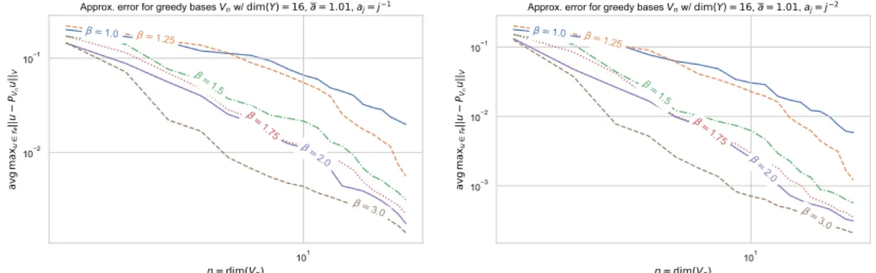
In our numerical test, we took 𝛿 = 10−2, that is ¯𝑎 = 1.01. As to the parametric dimension, we considered 𝑑 = 16 and 𝑑 = 64 that correspond to subdivisions of 𝐷 into 4 × 4 and 8 × 8 subdomains, respectively. As to the decay of 𝑎𝑗, we test the values 𝑡 = 1 and 𝑡 = 2. Finally for the growth of the training sample size 𝑁 (𝑛), we
test the values
𝛽 = 1, 1.25, 1.5, 1.75, 2. (5.5)
The error curves of the reduced basis approximation, averaged over 20 realizations of the random training sample, for the various choices of 𝑑, 𝑡 and 𝛽, are displayed on Figures1and2. The reduced basis approximation error has been computed by using separate test sample of cardinality similar to that of the training sample.
As predicted by the theoretical approximation results, the convergence rate of the reduced basis method improves as 𝑡 gets larger. The observed convergence rates (for the highest value of 𝛽) are closer to the value 𝑡 than to 𝑡 − 1/2 which can be rigourously established from the polynomial approximation rates. This reflects the fact that the reduced basis approximations perform generally better than sparse polynomial approximations.
Figure 1. Reduced basis approximation with 𝑑 = 16 and decay rate 𝑡 = 1 or 𝑡 = 2.
Figure 2. Reduced basis approximation with 𝑑 = 64 and decay rate 𝑡 = 1 or 𝑡 = 2.
We also note that, for the same value of 𝑡, the errors are smaller in the higher parametric dimension 𝑑 = 64 than for 𝑑 = 16. This apparent paradox can be explained: in both cases, the most active variables are the first ones (𝑦1, then 𝑦2, . . .) yet they are associated to domains 𝐷𝑗 of smaller size in the high dimensional case,
therefore having less impact on the variation of the solution with these variables.
As expected, we observe that the error curve behaves better as we increase the value of 𝛽 but we observed that this phenomenon stagnates at 𝛽 = 2. This hints that the scaling 𝑁 (𝑛) = 𝑛2 is practically sufficient to
ensure in this case the optimal convergence behaviour which would be met with a very rich training set, for example an 𝜀-net. The value 𝛽 = 2 is much smaller than the value 𝛽* given by the theoretical analysis which is
thus too pessimistic.
Acknowledgements. This research was supported by the ONR Contracts N00014-11-1-0712, N00014-12-1-0561, and N00014-15-1-2181; the NSF Grants DMS 1222715, DMS 1720297, DMS 1222390, and DMS 1521067; the Institut Uni-versitaire de France; The European Research Council under grant ERC AdG 338977 BREAD; and by the SmartState and Williams-Hedberg Foundation.
References
[1] M. Bachmayr, A. Cohen and G. Migliorati, Sparse polynomial approximation of parametric elliptic PDEs. Part I: affine coefficients. ESAIM: M2AN 51 (2017) 321–339.
[2] P. Binev, A. Cohen, W. Dahmen, R. DeVore, G. Petrova and P. Wojtaszczyk, Convergence rates for greedy algorithms in reduced basis methods. SIAM J. Math. Anal. 43 (2011) 1457–1472.
[3] A. Buffa, Y. Maday, A.T. Patera, C. Prud’homme and G. Turinici, A priori convergence of the Greedy algorithm for the parameterized reduced basis. ESAIM: M2AN 46 (2012) 595–603.
[4] A. Chkifa, A. Cohen, G. Migliorati, F. Nobile and R. Tempone, Discrete least squares polynomial approximation with random evaluations – application to parametric and stochastic elliptic PDEs. ESAIM: M2AN 49 (2015) 815–837.
[5] A. Chkifa, A. Cohen and C. Schwab, Breaking the curse of dimensionality in sparse polynomial approximation of parametric PDEs. J. Math. Pures Appl. 103 (2015) 400–428.
[6] A. Cohen and R. DeVore, Approximation of high-dimensional PDEs. Acta Numer. 24 (2015) 1–159.
[7] A. Cohen, R. DeVore and C. Schwab, Analytic regularity and polynomial approximation of parametric and stochastic PDEs. Anal. Appl. 9 (2011) 11—47.
[8] A. Cohen and G. Migliorati, Multivariate approximation in downward closed polynomial spaces. In: Contemporary Computa-tional Mathematics – A Celebration of the 80th Birthday of Ian Sloan. Springer, Cham (2018) 233–282.
[9] R. DeVore, G. Petrova and P. Wojtaszczyk, Greedy algorithms for reduced bases in Banach spaces. Constr. Approx. 37 (2013) 455–466.
[10] Y. Maday, A.T. Patera and G. Turinici, A priori convergence theory for reduced-basis approximations of single-parametric elliptic partial differential equations. J. Sci. Comput. 17 (2002) 437–446.
[11] Y. Maday, A.T. Patera and G. Turinici, Global a priori convergence theory for reduced-basis approximations of single-parameter symmetric coercive elliptic partial differential equations. C. R. Acad. Sci. Paris S´er. I Math. 335 (2002) 289–294.
[12] A.T. Patera, C. Prudhomme, D.V. Rovas and K. Veroy, A posteriori error bounds for reduced-basis approximation of parametrized noncoercive and nonlinear elliptic partial differential equations. In: Proc. 16th AIAA Computational Fluid Dynamics Conference (2003).
[13] G. Pisier, The Volume of Convex Bodies and Banach Spaces Geometry. Cambridge University Press (1989).
[14] G. Rozza, D.B.P. Huynh and A.T. Patera, Reduced basis approximation and a posteriori error estimation for affinely parametrized elliptic coercive partial differential equations application to transport and continuum mechanics. Arch. Com-put. Methods Eng. 15 (2008) 229–275.
[15] S. Sen, Reduced-basis approximation and a posteriori error estimation for many-parameter heat conduction problems. Numer. Heat Transfer B-Fund 54 (2008) 369–389.