HAL Id: hal-01298987
https://hal.sorbonne-universite.fr/hal-01298987
Submitted on 20 Apr 2016HAL is a multi-disciplinary open access archive for the deposit and dissemination of sci-entific research documents, whether they are pub-lished or not. The documents may come from teaching and research institutions in France or
L’archive ouverte pluridisciplinaire HAL, est destinée au dépôt et à la diffusion de documents scientifiques de niveau recherche, publiés ou non, émanant des établissements d’enseignement et de recherche français ou étrangers, des laboratoires
Structural stability of Lattice Boltzmann schemes
Claire David, Pierre Sagaut
To cite this version:
Claire David, Pierre Sagaut. Structural stability of Lattice Boltzmann schemes. Physica A, Elsevier, 2016, 444, pp.1-8. �10.1016/j.physa.2015.09.089�. �hal-01298987�
Structural stability of Lattice Boltzmann schemes
Claire David †, Pierre Sagaut ‡ October 17, 2015
† Université Pierre et Marie Curie-Paris 6
Laboratoire Jacques Louis Lions - UMR 7598
Boîte courrier 187, 4 place Jussieu, F-75252 Paris cedex 05, France
‡Université Aix-Marseille
ST JEROME, Avenue Escadrille Normandie Niemen 163 Avenue de Luminy, case 901 13009 Marseille, France
Abstract
The goal of this work is to determine classes of traveling solitary wave solutions for Lattice Boltzmann schemes by means of an hyperbolic ansatz. It is shown that spuri-ous solitary waves can occur in finite-difference solutions of nonlinear wave equation. The occurence of such a spurious solitary wave, which exhibits a very long life time, results in a non-vanishing numerical error for arbitrary time in unbounded numeri-cal domain. Such a behavior is referred here to have a structural instability of the scheme, since the space of solutions spanned by the numerical scheme encompasses types of solutions (solitary waves in the present case) that are not solutions of the original continuous equations. This paper extends our previous work about classical schemes to Lattice Boltzmann schemes ([1], [2], [3],[4]).
Key Words:
Lattice Boltzmann schemes; solitary waves; structural stability.
AMS Subject Classification: 65 M06, 65M12, 65M60, 35B99.
1
Introduction:
The lattice Boltzmann method (LBM ) is used for the numerical simulation of physical phenomena, and serves as an alternative to classical solvers of partial differential equa-tions. The primary domain of application is fluid dynamics; it is specially used to obtain the numerical solution of the incompressible, time-dependent Navier-Stokes equation.
The strength of the Lattice Boltzmann method is due to its ability to easily repre-sent complex physical phenomena, ranging from multiphase flows to fluids with chemical reactions. The principle is to "mimic" at a discrete level the dynamics of the Boltz-mann equation. Since it is based on a molecular description of a fluid, the knowledge of the microscopic physics can directly be used to formulate the best fitted numerical model. This method can be regarded as either an extension of the lattice gas automaton (LGA) [5], [6], [7], or a special discrete form of the Boltzmann equation from kinetic theory. Although the connection between the gas kinetic theory and hydrodynamics has long been established, the Lattice Boltzmann method (LBM ) needs additional special dis-cretization of velocity space to recover the correct hydrodynamics. Due to the very same reason, the LBM works exactly opposite traditional CFD methods in deriving working schemes: LBM uses Navier-Stokes equations as its target while traditional CFD methods use Navier-Stokes equations as their starting point.
Until a few years, the LBM was applicable to the isothermal flow regime, i.e., the weakly compressible, low-Mach-number limit. This flow regime is traditionally treated as "incompressible", although there are CFD methods constructed to compute the Navier-Stokes equations in this regime. The argument for treating very low-Mach-number flows as incompressible is pragmatic rather than physical. The direct calculation of the isother-mal Navier-Stokes equations requires time steps sufficiently sisother-mall to resolve acoustic waves across a computational cell. This time step may be vastly smaller than the time scales of interest for the bulk fluid motion. Thus the computational cost of the many additional time steps required by an isothermal calculation may be vastly higher than the cost of an incompressible calculation. Of course, in reality there is no fluid or flow that is absolutely incompressible (i.e., with infinite acoustic velocity). Recent works have shown that it is possible to define lattices able to overcome this limitation (see, for instance, [8], where the authors lay the theoretical foundation of the lattice Boltzmann model for the simulation of flows with shock waves and contact discontinuities, also [9], where one can find a pow-erful scheme the computational convergence rate of which can be improved compared to classical previous ones, while proving to be efficient for Taylor vortex flow, Couette flow, Riemann problem).
As for the enhancement of stability, which used to be pointed out in most lattice Boltzmann models, the regularization technique has been successfully shown as an efficient method of stabilization of the Single-Relaxation-Time (SRTLB) (see [10], where the model proposed by the authors enables one to raise significantly the maximum Reynolds number that could be simulated at a given level of grid resolution, in two and three dimensions).
2
The Lattice Boltzmann method
The lattice Boltzmann (LB ) method follows the same idea as its predecessor the Lattice Gas Automata (LGA) when it also considers the fluid on a lattice with space and time discrete. Instead of directly describing the fluid by discrete particles and, thus Boolean variables, it describes the fictitious system in terms of the probabilities of presence of the fluid particles. A lattice Boltzmann numerical model simulates the time and space evo-lution of kinetic quantities, the particle distribution functions fj(⃗r, t), 06 j 6 J, J ∈ N⋆.
The lattice Boltzmann equation is obtained by ensemble averaging the equation
⟨Nj(⃗r + ∆ t ⃗vj, t + ∆ t)⟩ = ⟨Nj(⃗r, t)⟩ + ⟨Ωj(N )⟩ (1)
where⟨Nj(⃗r, t)⟩ denotes the average number of particles at space position ⃗r and time t.
The system is supposed to satisfy the Boltzmann molecular chaos hypothesis, i.e. the fact that there is no correlation between particles entering a collision. Thus, the collision operator can be expressed as ⟨Ωi(N )⟩ = Ωi⟨N⟩, which leads to the Lattice Boltzmann
equation:
fj(r + ∆ t vj, t + ∆ t) = fj(r, t) + Ωj(f ) (2)
where, for j ∈ N, fj =⟨Nj⟩ denotes the probability to have a fictitious fluid particle of
velocity vj entering lattice site ⃗r at time t. The fj are also called the fluid fields, or the
particle distribution functions.
The collision operator is normally a non-linear expression and requires a lot of com-putation time [16]. In a big lattice, e.g. 3D model, the comcom-putation becomes impossible even on a massively parallel computer. To overcome this problem, Higuera et al. [11], [12] proposed to linearize the collision operator around its local equilibrium solution to reduce the complexity of the operation. Using this idea, Bhatnagar, Gross and Krook introduced the BGK lattice (LBGK ) [13], in which the collision between particles is de-scribed in terms of the relaxation towards a local equilibrium distribution. The LBGK is considered to be one of the simplest forms of the Lattice Boltzmann equation and is mathematically expressed as fj(⃗r + ⃗ejt + ∆t) = fj(⃗r, t)− 1 τ { fj(⃗r, t)− fjeq(⃗r, t) } j ∈ {0, . . . , J}, J ∈ N⋆ (3) where τ is the single relaxation time, which is a free parameter of the model to determine the fluid viscosity, and fjeq, j0, . . . , J , denote the local equilibrium functions, which are functions of the density and the flow velocity ⃗u.
In the lattice Boltzmann method, the space variable vector ⃗r is supposed to live in a
The velocity belongs to a finite set V composed by given velocities ⃗ej, j ∈ {0, . . . , J},
J ∈ N⋆, chosen in such a way that
⃗
r ∈ L and⃗ej ∈ V ⇒ ⃗r + ∆ t⃗ej ∈ L (4)
where ∆ t denotes the time step.
The set of velocitiesV is supposed to be invariant by space reflection, i.e.:
⃗ej ∈ V ⇒ ∃ l ∈ V : ⃗el=−⃗ej ∈ V (5)
The numerical scheme is thus defined through the evolution of the population fj(⃗r, t),
with ⃗r ∈ L and j ∈ {0, . . . , J} towards a distribution fj(⃗r, t + ∆ t) at a new discrete
time.
The scheme has two steps that take into account successively the left and right hand sides of the Boltzmann equation (1). The first step describes the relaxation of particle distribution towards the equilibrium. It is local in space and nonlinear in general. The second step is the collision process. Both steps have to be computed separately.
In general LB model, denoted by DdQ(J + 1), J ∈ N⋆, the actual macroscopic density,
which is function of the space vector ⃗r, and the time variable t, is obtained as a summation
of the microscopic particle distribution functions:
ρ(⃗r, t) =
J
∑
j=0
fj(⃗r, t) (6)
The macroscopic velocity is calculated as the average of the microscopic velocities ⃗ej,
j = 0, . . . , J , weighted by the related distribution functions:
⃗u(⃗r, t) = 1 ρ(⃗r, t) J ∑ j=0 fj(⃗r, t) ⃗ej (7)
In each time step, in each node, particles are streamed on to the neighbouring nodes, which thus lead to new distribution functions fj∗:
fj(⃗r + ⃗ei∆t, t + ∆t) = fj∗(⃗r, t + ∆t) , j = 0, . . . , J (8)
Also, once in each time step, the particles in each node collide, which is modeled as a relaxation of the distribution functions towards the equilibrium distributions
fj∗(⃗r, t + ∆t) = fj(⃗r, t) + 1 τ ( fjeq(⃗r, t)− fj(⃗r, t) ) (9) with: fjeq(⃗r, t) = ρ(⃗r, t) wj [ 1 +⃗ej· ⃗u(⃗r, t) c2 s +(⃗ej· ⃗u(⃗r, t)) 2 c4 s −(⃗u(⃗r, t)· ⃗u(⃗r, t))2 2 c2 s ] , j = 0, . . . , J
where cs is the lattice sound speed, such that: c2s = J ∑ j=0 wj⃗ej2
and where the weights wj, j = 0, . . . , J , are determined by the velocity set. Of course,
one has:
J
∑
j=0
wj = 1
The lattice Boltzmann equation takes both steps into account:
fj(⃗r + ⃗ei∆t, t + ∆t) = fj∗(⃗r, t + ∆t) = fj(⃗r, t) + 1 τ ( fjeq(⃗r, t)− fj(⃗r, t) ) , j = 0, . . . , J
The right-hand side gives thus the distribution of particles once collisions have occurred, while the left-hand side represents particles appearing in neighboring nodes in the next time step.
For our study, it is important to take into account the way the related algorithm is im-plemented:
i. Initialization step of ρ, ⃗u, and the microscopic densities fj, fjeq, j = 0, . . . , J .
ii. Streaming step: densities fj are moved towards fj∗ in the direction ⃗ej, j = 0, . . . , J ,
using (8).
iii. Computation step of the macroscopic variables ρ and ⃗u.
iv. Computation step of the microscopic variables fjeq, j = 0, . . . , J .
v. Collision step, in order to obtain the updated densities fj, j = 0, . . . , J , using (9).
3
Spurious lattice solitons
The discrete solution associated with the LB numerical scheme will admit spurious soli-tary waves, and therefore spurious local energy pile-up and local sudden growth of the error, if the discrete relation used to implement the scheme is satisfied by a solitary wave. Following [20], [1], [2], [3], [4], and using [21], [22], [23], [24], [25], [26], [27], [28], we search solitary waves solution components under the form:
ui(⃗r, t) = J ∑ j=0 { Ui,jsech [ kj ( xi− (⃗ej)i t )] + Vi,jtanh [ kj ( xi− (⃗ej)i t )]} (10) where ⃗ r = (xi)16i6d , ⃗ej = ( (⃗ej)i ) 16i6d , j = 0, . . . , J
and where Ui,j, Vi,j, kj, i = 1, . . . , d, j = 0, . . . , J , are real constants.
The question one may ask is how to switch from the scheme, which is discrete, to this continuous expression ? In so far as if one can find a solution of the above form (10) that fits each step of the scheme, is the answer. This is how we will proceed.
Starting from the fact that once the discrete populations fj are known, the main fluid
quantities can be obtained by simple linear summation upon the discrete speeds, it is legit-imate, for those densities, to be of the above form (10), for the same reasons as previously.
3.1 A one-dimensional example: the D1Q3 model
In the following, we examine a one-dimensional case, given by the flow of an incompress-ible fluid, in a domain [0, L], L > 0, obeying the Navier-Stokes equation, in order to test the D1Q3 model, which has a zero velocity and two oppositely directed ones, moving thus the fluid particle to the left and right neighbor lattice sites.
Figure 1:
The velocities are (see figure 1):
⃗e0 = ((⃗e0)x, 0) = ⃗0 , ⃗e1 = ((⃗e1)x, 0) = (1, 0) , ⃗e2 = ((⃗e2)x, 0) = (−1, 0)
while the weights are:
w0= 2 3 , w1 = 1 6 , w2 = 1 6 The conservation of mass quantity writes:
f1 = ρ u + f2 (11)
where u denotes the sole velocity component.
Since the density is a conserved quantity, we can suppose it to be constant, and nor-malized. In order to determine whether there exist, or not, solitary waves solutions, one requires to take into account related boundary conditions, in the case of an imposed ve-locity. Then, using (10), we search the densities fi, i = 1, 2, as functions of the horizontal
space variable x, and of the time one, t, under the form:
fi(y, t) = 2 ∑ j=0 { Φi,jsech [ kj ( x− (⃗ej)x t )] + Ψi,jtanh [ kj ( x− (⃗ej)x t )]}
and the horizontal velocity as:
u(x, t) = 2 ∑ j=0 { Ujsech [ kj ( x− (⃗ej)x t )] + Vjtanh [ kj ( x− (⃗ej)x t )]}
where, for j = 0, . . . , 2, kj, Φi,j, Ψi,j, Uj, Vj, are real constants to be determined.
By substituting those latter expressions in (11), one gets an equation of the form:
2 ∑
j=0
{
F (Φi,j, Ψi,j, Ux,j) sech
[
kj
(
y− (⃗ej)x t
)]
+Gi(Φi,j, Ψi,j, Vx,j) tanh
[ kj ( y− (⃗ej)x t )]} = 0
where we denote byF and G functions of Φi,j, Ψi,j, Uj, Vj. By independence of the terms
in sech and tanh, one gets, for j = 0, . . . , 2:
F (Φi,j, Ψi,j, Uj, Vj) = 0
G (Φi,j, Ψi,j, Uj, Vj) = 0
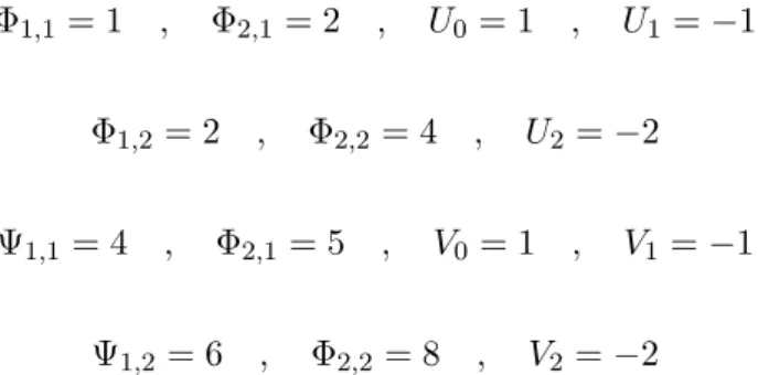
i.e. a linear system of two equations, the unknowns of which are the Φi,j, Ψi,j, Uj, Vj. It
Φ1,j = Uj+ Φ2,j , Ψ1,j = Vj+ Ψ2,j , j = 0, . . . , 2
which admits several sets of solutions. For sake of simplicity, we have chosen the following one:
Φ1,1 = 1 , Φ2,1= 2 , U0= 1 , U1=−1
Φ1,2 = 2 , Φ2,2= 4 , U2=−2
Ψ1,1 = 4 , Φ2,1= 5 , V0 = 1 , V1=−1
Ψ1,2 = 6 , Φ2,2 = 8 , V2 =−2
It thus exhibits the existence of lattice solitons, related to the discrete numerical scheme, of the form uni = AiSech [ ki(i h− n (⃗ej)i ∆ t) ] + BiTanh [ ki(i h− n (⃗ej)i ∆ t) ] , (Bi, ki) ∈ R2 (12)
Figure 2 displays the related lattice solitary wave, as a function of the mesh points ; nx
denotes the spatial number of mesh points in the x-direction, nt the time one.
3.2 A two-dimensional example: The case of an isothermal Poiseuille
flow between two parallel plates
The case of an isothermal Poiseuille flow, driven by a pressure gradient in the x-direction, between two horizontal, parallel, plates is an interesting one: if the flow is a two-dimensional one, yet, since it is a longitudinal one, one only has to deal with the lon-gitudinal velocity component, ux, which happens to depend only on the vertical space
variable y. In our case, that means that if there exists solitary waves, they also will be horizontal ones, and functions of y. Also, since the exact analytical expression of the velocity is known (the flow develops a parabolic velocity profile), results can be tested profitably. In the following, we will denote by H > 0 the distance between the two plates. The velocity vectors of the D2Q9 model are (see figure 3):
⃗ e0= ⃗0 = ( (⃗e0)x, (⃗e0)y ) = (0, 0)
Figure 2:
A "lattice solitary wave",
as a function of the mesh points, in the case of the D1Q3 model
⃗e1= ( (⃗e1)x, (⃗e1)y ) = (1, 0) , ⃗e2 = ( (⃗e2)x, (⃗e2)y ) = (0, 1) ⃗ e3 = ( (⃗e3)x, (⃗e3)y ) = (−1, 0) , ⃗e4 = ( (⃗e4)x, (⃗e4)y ) = (0,−1) ⃗e5 = ( (⃗e5)x, (⃗e5)y ) = (1, 1) , ⃗e6= ( (⃗e6)x, (⃗e6)y ) = (−1, 1) ⃗e7= ( (⃗e7)x, (⃗e7)y ) = (−1, −1) , ⃗e8 = ( (⃗e8)x, (⃗e8)y ) = (1,−1) In the specific case of the D2Q9 model, one has:
fjeq = wjρ ( 1 +3 ⃗ej · ⃗u c20 + 9 (⃗ej · ⃗u)2 2 c40 − 3 ⃗u2 2 c20 )
The weights of the population are given by:
w0 = 1 9 ∀ j ∈ {1, 2, 3, 4} : wj = 1 9 ∀ j ∈ {5, 6, 7, 8} : wj = 1 36
As in the above, in order to determine wether there exist, or not, solitary waves solutions, one requires to take into account related boundary conditions, in the case of an imposed
Figure 3:
Discrete velocity vectors of the D2Q9 model
velocity. We thus place ourselves in the case of the Zhou-He scheme [29]. The boundary between the fluid and the plates overlap the domain nodes. If one chooses to solve the undetermined population of the south boundary, ⃗e2, ⃗e5, ⃗e6, conservation of the mass and
quantity of movement yield: f2+ f5+ f6 = ρ− (f0+ f1+ f3+ f4+ f7+ f8) f5− f6 = ρ ux− (f1− f3− f7+ f8) f2+ f5+ f6 = f4+ f7+ f8 (13)
One can then use the bounceback of non-equilibrium in the direction normal to the wall:
f2− f2eq= f4− f4eq
which leads to:
f2 = f4 f5 = f7− f1− f3 2 + 1 2ρ ux f6 = f8+ f1− f3 2 − 1 2ρ ux (14)
Let us now study the existence of solitary waves solutions of (13) and (14). We assume the density to be constant, and normalized. Then, we search the densities fi, i = 0, . . . , 8,
and the longitudinal velocity component ux, as functions of the vertical space variable y,
fi(y, t) = 8 ∑ j=0 { Φi,jsech [ kj ( y− (⃗ej)x t )] + Ψi,jtanh [ kj ( y− (⃗ej)x t )]} ux(y, t) = 8 ∑ j=0 { Ux,jsech [ kj ( y− (⃗ej)x t )] + Vx,jtanh [ kj ( y− (⃗ej)x t )]}
where, for j = 0, . . . , 8, kj, Φi,j, Ψi,j, Ux,j, Vx,j, are real constants to be determined.
The boundary conditions on the plates require: ux(0, t) = 8 ∑ j=0 { Ux,jsech [ kj ( − (⃗ej)x t )] + Vx,jtanh [ kj ( − (⃗ej)x t )]} = 0 ux(H, t) = 8 ∑ j=0 { Ux,jsech [ kj ( H− (⃗ej)x t )] + Vx,jtanh [ kj ( H− (⃗ej)x t )]} = 0 (15) By substituting those latter expressions in (13) and (14), one gets a system of six equations of the form:
8 ∑
j=0
{
Fi(Φi,j, Ψi,j, Ux,j) sech
[
kj
(
y− (⃗ej)x t
)]
+Gi(Φi,j, Ψi,j, Vx,j) tanh
[ kj ( y− (⃗ej)x t )]} = 0
where, for i = 1, . . . , 6, we denote by Fi and Gi functions of Φi,j, Ψi,j, Ux,j, Vx,j. By
independance of the terms in sech and tanh, one gets, for i = 1, . . . , 6:
Fi(Φi,j, Ψi,j, Ux,j, Uy,j) = 0
Gi(Φi,j, Ψi,j, Ux,j, Uy,j) = 0
i.e. a linear system in 12 equations, the unknowns of which are the Φi,j, Ψi,j, Ux,j, Vx,j.
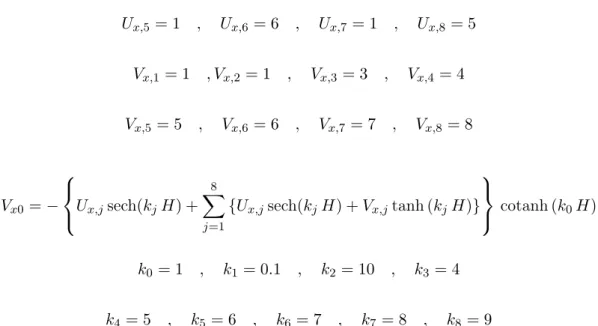
Taking into account the boundary conditions (15), resolution with a symbolic calculus tool (Mathematica for instance) shows that this system admits several sets of solutions. For sake of simplicity, we have choosen the following one:
Ux,0=−Ux,1− Ux,2− Ux,3− Ux,4− Ux,5− Ux,6− Ux,7− Ux,8
Ux,5= 1 , Ux,6= 6 , Ux,7 = 1 , Ux,8 = 5 Vx,1= 1 , Vx,2= 1 , Vx,3= 3 , Vx,4= 4 Vx,5= 5 , Vx,6= 6 , Vx,7= 7 , Vx,8= 8 Vx0=− Ux,jsech(kjH) + 8 ∑ j=1 {Ux,jsech(kjH) + Vx,jtanh (kjH)} cotanh (k0H) k0= 1 , k1 = 0.1 , k2 = 10 , k3= 4 k4 = 5 , k5= 6 , k6 = 7 , k7= 8 , k8 = 9
Figure 4 displays the related lattice solitary wave, as a function of the normalized vertical coordinate, which can be compared to the exact analytical solution.
4
Concluding remarks
The existence of spurious numerical lattice solitary waves for Lattice Boltzmann schemes has been proved. Such lattice solitary waves, which are not solutions of the exact contin-uous original equation, nevertheless satisfy the numerical scheme, appearing as parasitic solutions of the correct one. Such schemes will be referred to as structurally instable ones. A solution to avoid such spurious solitary waves, would be to "lock" the scheme by adding a test in the main loop.
Such spurious solitary waves have constant energy, and therefore the numerical error norm does not vanish at arbitrary long integration times on unbounded numerical domains.
One may ask why do such solutions occur ? A partial answer can be found in the equivalent continuous equation, the principle of which is the following: for a small time step ∆t, and the associated space scale h, a Taylor expansion in ∆t leads to establishing equivalent continuous equations as a formal limit. This matter has been explored by F. Dubois in [30], where it is proved that, at the first order in ∆t, the equivalent equation is the Euler equations, which are known to admit solitary waves solutions.
Figure 4:
A "lattice solitary wave",
in the case of a Poiseuille flow between two parallel plates (in red), compared with the analytical exact solution (dashed plot).
Acknowledgment
The authors would like to thank the anonymous referees, for their very judicious re-marks and advices, which helped improving the original work.
References
[1] Cl. David, P. Sagaut, Structural stability of discontinuous Galerkin schemes, Acta Applicandae, 113(1)1, 2011, 45-56.
[2] Cl. David, P. Sagaut, Structural stability of finite dispersion-relation preserving schemes, Chaos, Solitons and Fractals, 41(4), 2009, 2193-2199.
[3] Cl. David, P. Sagaut, Spurious solitons and structural stability of finite difference schemes for nonlinear wave equations, Chaos, Solitons and Fractals, 41(2), 2009, 655-660.
[4] Cl. David, R. Fernando, Z. Feng, A note on "general solitary wave solutions of the Compound Burgers-Korteweg-de Vries Equation", Physica A: Statistical and Theoretical Physics, 375 (1), 2007, 44-50.
[5] J. Hardy, Y. Pomeau and O. de Pazzis, Time Evolution of a Two-Dimensional Clas-sical Lattice System, PhyClas-sical Review Letters, 31, 1973, 276-279.
[6] D. d’Humières, P. Lallemand and U. Frisch, Lattice gas models for 3D-hydrodynamics, Europhysics Letters, 2(4), 1986, 291-297.
[7] U. Frisch, B. Hasslacher and Y. Pomeau, Lattice gas automata for the NavierŰStokes equation, Physical Review Letters, 56(14), 1986, 1505-1508, 1986.
[8] T. Kataoka and M. Tsutahara, Lattice Boltzmann method for the compressible Euler equations, Phys. Rev. E, 69(5), 2004, 056702-1–056702-1-14.
[9] Y. Wang, Y. L. He, T. S. Zhao, G. H. Tang and W. Q. Tao, Implicit-Explicit finite-difference Lattice Boltzmann method for compressible flows, International Journal of Modern Physics C, 18(12), 2007, 1961-1983.
[10] A. Montessori, G. Falcucci, P. Prestininzi, M. La Rocca, S. Succi, Regularized lat-tice Bhatnagar-Gross-Krook model for two-and three-dimensional cavity flow simu-lations, Phys. Rev. E, 89, 053317-1–053317-8.
[11] F. Higuera, J. Jimenez, and S. Succi. Boltzmann approach to lattice gas simulations, Europhys. Lett, 9, 1989, 663.
[12] F. Higuera, J. Jimenez, and S. Succi. Lattice Gas dynamics with enhanced collision. Europhys. Lett, 9, 1989, 345.
[13] P. Bhatnagar, E. Gross and M. Krook. ŞA Model for Collision Processes in Gases. I. Small Amplitude Processes in Charged and Neutral One-Component SystemsŤ, Physical Review, 94, 1954, 511-525.
[14] Y. Qian, D. d’Humières, and P. Lallemand, Lattice BGK models for Navier- Stokes equation, Europhys. Lett, 17, 1992, 470-84.
[15] D. d’Humières, Generalized Lattice-Boltzmann Equations, in Rarefied Gas Dynam-ics: Theory and Simulations, AIAA Progress in Astronautics and Astronautics, 1959, 1992, 450-458.
[16] B. Chopard, A. Dupuis, A. Masselot, and P. Luthi. Cellular Automata and Lat-tice Boltzmann techniques: An approach to model and simulate complex systems, Advances in Complex Systems, 5, 2002, 103-246.
[17] B. Chopard and M. Droz, Cellular Automata Modeling of Physical Systems, Cam-bridge University Press, 1998.
[18] M. B. Reider and J. D. Sterling, Accuracy of Discrete-Velocity BGK modor the simulation of the incompressible Navier-Stokes equations, Comput. fluids, 24(4), 1995, 459-467.
[19] P. Lallemand, L.-S. Luo, Theory of the lattice Boltzmann method: Dispersion, dis-sipation, isotropy, Galilean invariance, and stability, Physical Review E, 61, 2000, 6546-6562.
[20] Z. Feng, G. Chen, Solitary Wave Solutions of the Compound Burgers-Korteweg-de Vries Equation, Physica A, 352, 2005, 419-435.
[21] B. Li, Y. Chen Y. and H.Q. Zhang, Explicit exact solutions for new general two-dimensional KdV-type and two-two-dimensional KdV-Burgers-type equations with non-linear terms of any order, J. Phys. A (Math. Gen.), 35, 2002, 8253-8265.
[22] G. B. Whitham, Linear and Nonlinear Waves, Wiley-Interscience, New York, 1974. [23] M. J. Ablowitz, H. Segur, Solitons and the Inverse Scattering Transform, SIAM,
Philadelphia, 1981.
[24] R. K. Dodd, J.C. Eilbeck, J. D. Gibbon, H.C. Morris, Solitons and Nonlinear Wave Equations, London Academic Press, London, 1983.
[25] R.S. Johnson, A Modern Introduction to the Mathematical Theory of Water Waves, Cambridge University Press, Cambridge, 1997.
[26] E.L. Ince, Ordinary Differential Equations, Dover Publications, New York, 1956. [27] G. Birkhoff, G.C. Rota, Ordinary Differential Equations, Wiley, New York, 1989.
[28] A.D. Polyanin, V. F. Zaitsev, Handbook of Nonlinear Partial Differential Equations, Chapman and Hall/CRC, 2004.
[29] Q. Zou, and X. He, Pressure and velocity boundary conditions for the lattice Boltz-mann, J. Phys. Fluids, 9, 1997, 1591-1598.
[30] F. Dubois, Equivalent partial differential equations of a lattice Boltzmann scheme, Computers and Mathematics with Applications, 55, 2008, 1441Ű1449.