HAL Id: hal-01764525
https://hal.archives-ouvertes.fr/hal-01764525
Submitted on 12 Apr 2018
HAL is a multi-disciplinary open access archive for the deposit and dissemination of sci-entific research documents, whether they are pub-lished or not. The documents may come from teaching and research institutions in France or abroad, or from public or private research centers.
L’archive ouverte pluridisciplinaire HAL, est destinée au dépôt et à la diffusion de documents scientifiques de niveau recherche, publiés ou non, émanant des établissements d’enseignement et de recherche français ou étrangers, des laboratoires publics ou privés.
Pruning Infeasible Paths via Graph Transformations and
Symbolic Execution: a Method and a Tool
Romain Aissat, Marie-Claude Gaudel, Frédéric Voisin, Burkhart Wolff
To cite this version:
Romain Aissat, Marie-Claude Gaudel, Frédéric Voisin, Burkhart Wolff. Pruning Infeasible Paths via Graph Transformations and Symbolic Execution: a Method and a Tool. [Research Report] 1588, Laboratoire de Recherche en Informatique [LRI], UMR 8623, Bâtiments 650-660, Université Paris-Sud, 91405 Orsay Cedex. 2016. �hal-01764525�
L R I
CNRS – Université de Paris Sud
Centre d’Orsay
LABORATOIRE DE RECHERCHE EN INFORMATIQUE
Bâtiment 650
91405 ORSAY Cedex (France)
R
A
P
P
O
R
T
D
E
R
E
C
H
E
R
C
H
E
PRUNING INFEASIBLE PATHS VIA GRAPH
TRANSFORMATIONS AND SYMBOLIC
EXECUTION : A METHOD AND A TOOL
AISSAT R / GAUDEL M C / VOISIN F / WOLFF B
Unité Mixte de Recherche 8623
CNRS-Université Paris Sud-LRI
06/2016
Pruning Infeasible Paths via Graph Transformations
and Symbolic Execution: a Method and a Tool
Romain Aissat, Marie-Claude Gaudel, Frédéric Voisin, Burkhart Wolff
LRI, Univ Paris-Sud, CNRS, CentraleSupélec, Université Paris-Saclay, France [email protected]
Abstract—Path-biased random testing is an interesting alternative to classical path-based approaches faced to the explosion of the number of paths, and to the weak structural coverage of random methods based on the input domain only. Given a graph representation of the system under test a probability distribution on paths of a certain length is computed and then used for drawing paths. A limitation of this approach, similarly to other methods based on symbolic execution and static analysis, is the existence of infeasible paths that often leads to a lot of unexploitable drawings.
We present a prototype for pruning some infeasible paths, thus eliminating useless drawings. It is based on graph transformations that have been proved to preserve the actual behaviour of the program. It is driven by symbolic execution and heuristics that use detection of subsumptions and the abstract-check-refine paradigm. The approach is illustrated on some detailed examples.
I. INTRODUCTION
White-box, path-based, testing is a well-known tech-nique, largely used for the validation of programs. Given the control-flow graph (CFG) of the program under test, generation of a test suite is viewed as the process of first selecting a collection of paths of interest, then trying to provide, for each path in the collection, concrete values for the program parameters that will make the program follow exactly that path during a run.
For the first step, there are various ways to define what is meant by paths of interest: structural testing methods aim at selecting some set of paths that fulfills coverage criteria related to elements of the graph (vertices, edges, paths of given length, etc); in random-based techniques, paths are selected according to a given distribution of probability over these elements (for instance, uniform probability over all paths of length less than a given bound). Both approaches can be combined as in struc-tural statistical testing [1, 2]. The random-based methods above have the advantage of providing a way to assess
the quality of a test set as the minimal probability of covering an element of a criterion.
Handling the second step requires to produce for each path its path predicate, which is the conjunction of all the constraints over the input parameters that must hold for the system to run along that path. This is done using symbolic execution techniques [3]. Then, constraint-solving is used to compute concrete values to be used for testing the program. If for no input values the path predicate evaluates to true, the path is infeasible. It is very common for a program to have infeasible paths and such paths can largely outnumber feasible paths. Every infeasible path selected during the first step will not contribute to the final test suite, and there is no better choice than to select another path, hoping for its feasibility. Handling infeasible paths is the serious limitation of structural methods since such methods can spend most of the time selecting useless paths. It is also a major challenge for all techniques in static analysis of programs, since the quality of the approximations they provide is lowered by data computed for paths that do not exist at program runs.
To overcome this problem, different methods have been proposed, like concolic testing (see Section VII) or random testing based on the input domain [4]. In path-biased random testing, paths in the CFG are drawn according to a given distribution and checking the fea-sibility of paths is done in a second step. In [5], for each drawing yielding an infeasible path, a new path was drawn, while trying to learn infeasibility patterns from the set of rejected paths. But the experimental results were not satisfactory for programs with many infeasible paths. Here, we follow another approach, namely we present a prototype that builds better approximations of the behavior of a program than its CFG, providing a transformed CFG, which still over-approximates the set of feasible paths but with fewer infeasible paths. This transformed graph is used for drawing paths at random.
In [6] we modelled our graph transformations and formally proved the two key properties that establish the correctness of our approach: all feasible paths of the original CFG have counterparts in the transformed graph, and to each path in the new graph corresponds a path in the original CFG performing the same computations.
Our algorithm uses symbolic execution of the paths in the CFG, which, in conjunction with constraint solving, allows to detect whether some paths are infeasible. As programs can contain loops, their graphs can contain cycles. In order to avoid to follow infinitely a cyclic path, we enrich symbolic execution with the detection of subsumptions. Roughly speaking, a subsumption can be interpreted as the fact that some node met during the analysis is a particular case of another node met previously. As a result, there is no need to explore the successors of the subsumed node: they are subsumed by the successors of the subsumer.
The paper is organized as follows. In Section II we recall classical definitions, and introduce the basic oper-ations performed by the algorithm: symbolic execution, detection of subsumption, and abstraction. In Section III, we present our main algorithm and its heuristics before describing in Section IV, how it behaves on an example. Section V shows experimental results on three examples. Section VI briefly reports about proving the correctness of the approach. Finally, we present related works in Section VII and conclude in Section VIII.
II. BACKGROUND
A. Modelling programs
Programs are modelled by labelled transition systems (LTS). A LTS is a quadruple (L, l0, ∆, F ) where L is
the set of program locations, l0 ∈ L is the entry point of
the program and F ⊆ L the set of final vertices, i. e. exit points. ∆ ⊆ L×Labels×L is the transition relation, with Labels being a set of labels whose elements represent the basic operations that can occur in programs.
In this paper, a label can be as follows:
• Skip, used for edges associated with break, continue
or jump statements,
• Assume φ, where φ is a boolean expression over
Vars, the set of program variables,
• Assign v e, where v is a program variable and e an
expression over elements of Vars.
Vertex l0 has no incoming edge and elements in F
have no outgoing edges. In the underlying graph, all
vertices are reachable from l0 and reach an element in
F.
The transition relation represents the operations that are executed when control flows from a program location to another. We write l label
→ l0 to denote the transition leading from l ∈ L to l0
∈ L executing the operation corresponding to label ∈ Labels.
Conditional statements are directly encoded using the underlying graph structure of the LTS by adding edges labelled with the condition to the successors.
Such LTS model programs as if they were the result of a pre-compiler for a simple imperative programming language where basic operations are either assignments or Skip; Conditional statements are either If-Then-Else blocks (the Else-branch being optional) or While-loops. There is no explicit block structure as it is assumed that, after some scope analysis and renaming, all variables are defined at the topmost level. We call D the domain of program variables. A program state is a function σ : Vars → D. In the following examples, we assume D to be the set of integers. This could be extended to arrays, records and other constructs. Actually, the approach presented here can be combined with existing memory models such as [7, 8]: this leads to consider new kinds of formulae, but the notions of subsumption and abstraction will remain relevant. The real limit comes from the constraint solver in use.
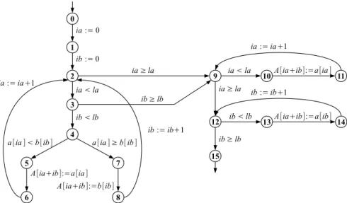
In Figure 1, we give the LTS for a program that merges two sorted arrays. Its input are two arrays a and b of integers and their respective lengths la and lb. It returns a third array A containing the elements of a and b, sorted in ascending order. The program code is made essentially of three loops. The first one iterates on both a and b, and stores their elements in A until one of the two arrays is exhausted. The array that has not been completely traversed is then processed by one of the last two loops. Although simple, this program contains a lot of infea-sible paths, assuming no pre-condition about la or lb. We distinguish seven "groups" of infeasible paths, and five of feasible paths (one group with a single path). For example, any path going through 2 ia≥la→ 9 (resp. 3ib≥lb→ 9) then 9ia<la→ 10 (resp. 12ib<lb→ 13) is infeasible. Also, any feasible path can enter at most one of the last two loops and not entering either loop is feasible only when the input arrays are empty. We do not detail the other groups, but in the case of merging sort, the reason of infeasibility generally lies in the fact that a and b cannot have been both completely visited when the execution exits the first loop.
1 2 0 3 9 10 11 12 15 5 7 6 8 4 A[ia+ib]:=a[ia ] ia := 0 ib := 0 ia ≥ la ib ≥ lb ia < la ib < lb
a[ia ] < b[ib ] a[ia ] ≥ b[ ib ]
A[ia+ib]:=b[ib] ia := ia+1 ib := ib+1 ia < la ia := ia+1 A[ia+ib]:=a[ia ] ia ≥ la ib ≥ lb 13 14 ib < lb ib := ib+1 A[ia+ib]:=a[ib]
Figure 1: The LTS for the merging sort algorithm. B. Symbolic Execution
A symbolic variable is an indexed version of a pro-gram variable. The set Vars×N of all symbolic variables is denoted SymVars.
Symbolic execution performs over configurations, which are pairs (s, π). The first member s, the store, is a function from program variables to indexes which maps program variables to symbolic variables. The second member π, the path predicate, is a formula over symbolic variables which is the conjunction of constraints met during symbolic execution. The set of all configurations is denoted by C. A configuration is satisfiable if and only if its path predicate is satisfiable.
We represent symbolic execution by a function SE : C× Labels → C, and define it as follows:
SE c l = c if l = Skip (s, π∧ φs) if l = Assume φ (s0, π∧ (v, s0(v)) = es) if l = Assign v e where:
• es (resp. φs) denotes the expression obtained from
e (resp. φ) by substituting every occurrence of a program variable v by (v, s(v)),
• s0 is obtained by updating s in such a way that the
symbolic variable (v, s0(v))is fresh1 for c.
C. Subsumption
Subsumption is a relation between configurations. Informally, a configuration c is subsumed by a
configu-1i.e. it is not yet associated to a program variable by the store and
it does not occur in the path predicate.
ration c0 if it is a particular case of c0. More precisely, a
configuration represents a set of program states and c is subsumed by c0 if the set of program states represented
by c is a subset of the set of program states represented by c0. In the following, we define the concepts needed to
formalise this notion of program states represented by a configuration.
Given a store s, a program state σ : Vars → D and a symbolic state σsym : SymVars → D, σ and σsym are
said to be consistent with s, noted cons(s, σ, σsym), if
∀ v ∈ Vars. σ(v) = σsym((v, s(v)))
Given an arithmetic or boolean expression e over program (resp. symbolic) variables and a program state σ (resp. a symbolic state σsym), we write e(σ) (resp.
e(σsym)) the evaluation of e in σ (resp. in σsym).
The set of program states represented by a configura-tion c = (s, π), or simply the set of states of c, denoted States(c), can then be defined in the following way:
States(c) ={σ. ∃ σsym. cons(s, σ, σsym)∧ π(σsym)}
If the path-predicate of a configuration is unsatisfiable, its set of states is empty.
A configuration c is subsumed by another configura-tion c0, noted c v c0, if States(c) ⊆ States(c0).
Symbolic execution is monotonic with respect to this definition of subsumption. There is no need to explore the successors of a subsumed point, as they are subsumed by the successors of the subsumer. It follows that the set of feasible paths starting at the subsumee is a subset of the set of feasible paths starting at the subsumer [6].
Therefore, as subsumption corresponds to an inclu-sion of paths, adding a subsumption to the symbolic execution tree often comes at the price of introducing infeasible paths into it. A challenge is thus to accept only subsumptions that introduce a reasonable number of infeasible paths. This is addressed in section III. D. Abstraction
Unfolding loops by symbolic execution in a LTS may yield an infinite symbolic execution tree. To get a finite representation, loops must be subject to subsumption at some point. Every time a loop header is reached when extending a symbolic execution path, the algorithm checks if a subsumption can apply with one of the previous occurrences of the same loop header on the path. The configurations at the subsumer and subsumee record two snapshots of the (symbolic) values of vari-ables along that path, as given by the store and the path predicate. Except for trivial loops, the symbolic values of some variables have changed between the configura-tions and subsumption might not occur. Abstracting a configuration means forgetting part of the information in the configuration at the subsumer for forcing the subsumption. The store component of a configuration merely records the symbolic variable currently associated with a program variable; in the path predicate constraints over symbolic variables are expressed as conjunctions of formulae on symbolic variables, reflecting decisions and assignments that take place along the path. Abstraction discards some of these formulae and there are various ways to do so: remove a set of conjuncts, or compute a weaker form of the path predicate that would be implied by the current path predicates of both configurations, see for instance [9, 10]. Abstraction at a loop header amounts to compute some kind of invariants for that loop.
Once abstraction has been performed for the sub-sumer, configurations located in its subtree must be recomputed by propagating the abstract configurations to the successors. Propagating the abstraction could rule out existing subsumptions involving successors of the subsumer. Moreover, it must also be checked that the abstraction propagated to the subsumee is now subsumed by the abstracted subsumer, which is not guaranteed. When such a conflict exists, we keep the existing sub-sumptions and discard the abstraction.
When no abstraction is retained with any of the previ-ous occurrences on the path of the same loop header, the loop is unfolded again by symbolic execution, hoping for a future subsumption.
Forcing a subsumption with an abstraction is not
always profitable: each abstraction discards part of in-formation about the current symbolic values of variables at that program point and possibly add a whole set of new infeasible paths, in comparison to the set of feasible paths one would have obtained with classical symbolic execution. In Section III we describe how our heuristics limit that problem. A crucial point for limiting the unfolding of loops without introducing infeasible paths is the choice of the predecessor with which to subsume and of the abstraction that makes it possible. E. Limiting Abstractions
To prevent from performing unwanted abstractions at a configuration, or for recording that some abstraction has been banned by some kind of counterexample driven refinement [10], predicates can be attached to configu-rations for loop headers. They act as safeguard against too crude abstractions: only abstract configurations that imply the additional predicate will be considered. This predicate is usually obtained after some kind of refine-ment. In Section III we use a weakest-precondition calcu-lus for that purpose. To make sure that no feasible path is discarded by attaching the predicate to a configuration, the predicate must hold for all states described by the configuration. This additional predicate is not part of the configuration and is not propagated to successors.
III. ALGORITHM
Our algorithm transforms a given CFG into one with fewer infeasible paths. It takes an LTS S and an initial configuration c as inputs, and produces a new LTS S0.
In [6] we have formally proved that S0 fulfills the two
following properties: (i) for every path in S0 there exists
a path with the same trace in S; (ii) for every feasible path of S starting with the initial configuration c, there exists a path with the same trace in S0.
A. Red-Black Graphs
The algorithm builds an intermediate structure that we call a red-black graph, which is turned back into a LTS when the analysis is over. A red-black graph RB is a 6-uple (B, R, S, C, M, Φ) where:
• B = (L, l0, ∆, F ) is the input LTS that we call the
black part. It is never modified during the analysis,
• R = (V, r, E) is a rooted graph (a LTS without
labels) that we call the red part, which represents the symbolic execution tree built so far and can be seen as a partial unfolding of the black part; V ⊆ L × N is its set of vertices, called the red vertices; they are indexed versions of elements of
L representing occurrences of locations of B met during the analysis; r ∈ V is its root; E ⊆ V ×V is its set of edges. Function fst returns the first element of a couple; we use it to retrieve the black vertex associated with a red vertex,
• S ⊆ V ×V is the subsumption relation between red
vertices computed so far,
• C is a function from red vertices to configuration
stacks: a red vertex can have multiple configurations (reflecting different choices of abstraction) during the analysis and we need to keep track of these configurations. In the following, given a red vertex rv, we call configuration of rv the configuration on top of the stack associated with rv,
• M, the marking, is a function from red vertices to
boolean values recording partial information about unsatisfiability: given a red vertex rv, M(rv) is true only if the configuration of rv has been proved unsatisfiable. A constraint solver is used for that purpose (assumed to be correct, but not complete). For performance reasons, it is not called upon every vertex. If M(rv) is false, then rv has been proved satisfiable or nothing is known about its satisfiability and it is treated as if it is satisfiable. Symbolic execution stops at vertices for which M holds. Hence, no element in V is a successor of such vertex,
• Φ is a function from red vertices to formulae over
program variables recording the predicates used for limiting abstractions (see Section II-E).
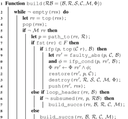
We give the pseudo code of the main parts of the algorithm in Figures 2 and 3. The algorithm maintains a global data structure rvs of red vertices to visit. In the current version, rvs is a stack built according to a DFS traversal of the LTS. It starts with the original LTS and an initial configuration c whose store maps each program variable to a symbolic variable and whose path predicate is a user-provided formula (precondition of the program under test). In practice this formula must belong to the logic supported by the constraint solver, as must do the formulae of the Assume transitions in the LTS.
B. Building the Red-Black Graph
The main function, build (Figure 2), is a loop that runs until there are no more red vertices to visit in the stack rvs, in which case the analysis is complete.
Initialization: When the analysis starts, build is called with RB in the following initial state:
• B is S, the LTS under analysis,
• the root r of R is the couple (l0, 0), which is also
the only element of V ,
• E and S are empty, since the red graph is empty, • C associates with r a one-element stack that
con-tains the initial configuration c,
• M associates false with r, • Φassociates true with r,
and rvs contains r only.
If the stack rvs is not empty (line 2), its first element, called rv, is popped. If the configuration of rv is marked (line 5), i.e. it is known to be unsatisfiable (thanks to a call to a constraint solver), the symbolic execution halts along that path. Otherwise, the path p leading from r to rv in R is recovered (modelled by the primitive path_to at line 6).
Symbolic execution: this is the nominal action when none of the special cases detailed below apply: it per-forms a partial unfolding of R by a symbolic execution step at rv (lines 17, 19). We explain here how M, C and Φ propagate to the immediate successors.
For every transitions (fst rv)label
→ l in ∆:
• the edge (rv, (l, i)) is added to E, where i is a fresh
index for location l,
• the configuration SE (top (C rv)) label (see
Sec-tion II-B) is pushed on C (l, i),
• if label is of the form Assume φ, with φ being
false2, then (l, i) is marked in M. If φ is neither
false nor true, then a constraint solver is called to check the satisfiability of the new configuration: (l, i)is marked in M only if the solver proves it is unsatisfiable (as for the case of subsumption),
• Φis updated such that it associates true with (l, i).
Successors are then pushed onto rvs in order to be processed in the next iterations of the loop.
Handling final locations and limiting abstractions: If rv is an occurrence of a final location of B (line 7), the algorithm checks the infeasibility of p from the initial configuration (call ifp to a solver at line 8). If p turns out to be infeasible, it could come from one of the abstractions made along p, at some red vertex rv0, resulting in a loss of information about the
program state that caused p to be considered feasible. A "refine-and-restart" phase is triggered. The refine-part consists in searching such rv0 along p, which is done by
faulty_abs(line 9). We do not give its pseudo code,
2In this paper this would occur only in case of a loop or conditional
but the idea is to search back in p the red vertex rv0
whose stack of configurations contains two (consecutive) configurations ci and cj such that the suffix of p starting
at rv0 is infeasible from c
i but was feasible from cj:
configuration cj corresponds to the faulty abstraction.
In lines 10 and 11, the algorithm computes a condition that will block any attempt to build p again. Let p0 be
the subpath of p going from rv0 to its first successor in
p whose configuration is unsatisfiable: the condition φ returned by ifp_cond is the weakest precondition of false w.r.t. to the trace of p0. φ is then joined to Φ(rv0).
Next, the configuration of rv0 prior to the faulty
ab-straction is restored (line 12) and its subtree is destroyed (line 13), i.e. RB is updated in the following way:
• configuration stacks of successors of rv0 are
re-moved from C,
• subsumptions involving rv0 or any of its successor
are removed from S,
• successors of rv0 marked in M are unmarked, • entries of Φ involving successors of rv0 are
re-moved,
• every edge starting or ending in a successor of rv0
is removed from E,
• and every successor of rv0 is removed from rvs.
Finally, rv0 is pushed on rvs so that the analysis restarts
at rv0, now strengthened with φ, for the next iteration of
the loop in build.
In our prototype, the whole refine-restart part is con-troled by a user switch: without it, when a final vertice is reached the algorithm simply selects the next vertex to visit in rvs; building the final LTS is faster but it often keeps many infeasible paths because of loose ab-stractions. With it, the risk is that no better abstraction is found and the loop is unfold once more without guaranty about finding a better situation at the next occurrence of the loop header, yielding a possible infinite chain of unfoldings. This is due to the fact that our method of abstracting does not learn from the safeguard condition: the subsumption is postponed in the hope that a more accurate abstraction can be found later. A compromise is to keep the refine-restart and bound the maximal length of paths or unfoldings, but experimenting with learning abstraction methods is definitely worth doing.
Finding abstraction: Suppose that rv is an occurrence of a loop header (line 15), the algorithm attempts at detecting a subsumption of rv with a red vertex, for the same black location, previously met along p (line 16). Function subsumed (Figure 3) iterates over the vertices of p. When an occurrence rv0 for the same black vertex
is found (line 22), the constraint solver is called to check if the configuration of rv0 subsumes the one at rv (line
23). If yes, the subsumption is established and (rv, rv0)
is added to S (line 24). If the answer is negative or unknown3, function abs (line 26) attempts at abstracting
the configuration of rv0 in order that i) it subsumes the
configuration of rv and ii) it entails Φ(rv0).
There are various ways to find such abstractions. The current version of abs replaces the first conjunct in the path predicate of the configuration of rv0 by true,
checks if Φ(rv0)is entailed then checks if the abstracted
configuration subsumes the configuration of rv. If this is the case, the abstracted configuration is returned. Otherwise, abs replaces the second conjunct (still using true in place of the first conjunct), and so on. If Φ(rv0)
is no longer entailed, the search for an abstraction is canceled. If Φ(rv0) still have its default value of true
and no better abstraction is found, we end up with a path predicate becoming equivalent to true and a trivial abstraction occurs.
The ability of the algorithm to eliminate infeasible paths depends on the precision of the way configurations are abstracted, and we plan to experiment with more precise methods of abstraction. In Section IV-B we present a heuristics based on a fixed lookahead of the feasiblity of the successors of the subsumed vertices. The current simple and greedy algorithm used by abs requires only a number of calls to the constraint solver that is linear in the initial number of conjuncts.
If an abstraction is returned by abs, it is checked that it can be propagated without invalidating existing sub-sumptions involving successors of rv0 (line 27). If this
is not the case, the subsumption at the loop header does not take place and the search for an abstraction halts, since a looser abstraction will not help here. Otherwise, the abstraction is propagated (line 28) by performing symbolic execution in the subtree with root rv0 with
the abstracted configuration pushed on its stack, and pushing newly computed configurations on the stacks of the successors of rv.
One can observe that depending on the order in which the LTS is traversed, a successor of rv0 can have been
al-ready abstracted (i.e. its stack of configurations contains more elements than the stack of rv0). To account for
both abstractions, the path predicate of the configuration pushed on its stack is the conjunct of all sub-formulae
3In the case of an unknown answer, accepting the subsumption
would result in a loss of feasible paths in the resulting LTS when the configuration of rv is not subsumed by the one at rv0.
1 Function build(RB = (B, R, S, C, M, Φ)) 2 while ¬ empty(rvs) do 3 let rv = top(rvs); 4 pop(rvs); 5 if ¬ M rv then 6 let p = path_to(rv, R); 7 if fst(rv) ∈ F then
8 if ifp(p, top(C r), B) then 9 let rv0= faulty_abs(p, C, B) 10 and φ = ifp_cond(p, rv0, B); 11 Φ rv0← Φ rv0∧ φ; 12 restore(rv0, p, C); 13 destroy(rv0, R, S, C, M, Φ); 14 push(rv0, rvs);
15 else if loop_header(rv, B) then 16 if ¬ subsumed(rv, p, RB) then 17 build_succs(rv, B, R, C, M);
18 else
19 build_succs(rv, B, R, C, M);
Figure 2: Building the symbolic execution tree. common to the path predicates of both abstractions (the two stores are identical).
Besides, propagating an abstraction can turn configu-rations back from unsatisfiable to satisfiable. Red vertices where this phenomenon occurs must be unmarked and pushed on the stack rvs.
Once the abstraction has been propagated, the new subsumption is added to S (line 29).
The algorithm may not terminate. Our implementation takes the maximal red length, noted mrl, of symbolic paths as an additional parameter. Whenever the current symbolic path reaches this bound, the algorithm is not allowed to extend it further (but it can attempt to trigger a refine-and-restart phase or to subsume it).
C. Building the new LTS
Once the analysis is over, RB is turned back into a new LTS S0 by removing from the red part R the edges
leading to marked red vertices, replacing the targets of edges leading to subsumed red vertices by their sub-sumers, then renaming vertices and label edges between red vertices with the label of the edge between their black counterparts. For red vertices where the analysis halted because of the mrl limit, if any, the edges whose target is not final are connected to the corresponding vertex in the black part, i.e. to the original CFG. This trick and the fact that transformations on the red part never rule out (prefixes of) feasible paths ensures that S0 preserves
the feasible paths of S.
IV. EXAMPLE:MERGING SORT
We now detail how our algorithm behaves in the case of merging sort. In this example, statements and conditions that use the values of the elements in arrays
20 Function subsumed(rv, p, RB = (B, R, S, C, M, Φ)) 21 foreach rv0∈ p do
22 if fst(rv0)= fst(rv)then
23 if top(C rv) v top(C rv0)then 24 S ← S ∪ {(rv, rv0)}; 25 return true;
26 if abs(rv0, rv, C, Φ) = Some(a) then 27 if can_prop(a, rv0, B, R, C, S) then 28 propagate(a, rv0, B, R); 29 S ← S ∪ {(rv, rv0)}; 30 return true; 31 return false;
Figure 3: Detecting a subsumption.
1 2 0 3 5 6 7 9 4 ia := 0 ib := 0 ia ≥ la ib ≥ lb ia < la ib < lb ia := ia+ 1 ib := ib+ 1 ia < la ia := ia+ 1 ia ≥ la ib ≥ lb 8 ib < lb ib := ib+ 1
Figure 4: Simplified LTS for the merging sort example. a, b and A have no influence at all on the feasibility of paths. In the following, we proceed with a slightly simplified and compacted version of the LTS of Figure 1, which is shown in Figure 4: subpaths 4 − 5 − 6 − 2 and 4− 7 − 8 − 2 in the CFG are replaced by two edges 4− 2 in the new LTS, with the labels of the two original edges 6 − 2 and 8 − 2. We suppose that at each traversal of the loop, any of these two edges can be chosen non-deterministically. Instead of a sort program we have a program traversing two arrays in an arbitrary way. Again, this change does not influence the set of infeasible paths which only depends on how indexes in input arrays vary. But it does impact time spent in the constraint-solver.
First, we show and interpret the result given by the algorithm as it was presented in Section III. Then, we show how to greatly improve this result using a simple heuristic that discards too crude subsumptions. In the following, we write li to denote the red vertex (l, i).
A. Merging sort without heuristic
Initialization: The analysis starts at red vertex 00
(Figure 5). We make no particular assumption over program variables: the initial configuration is ({ia 7→ ia0, ib7→ ib0, la7→ la0, lb 7→ lb0}, true).
Handling the first assignments: Symbolic execution is used for handling 00 then 10 before reaching vertex 20.
Execution of the body of the first loop: Here, both successors of 20, namely 30 and 50, are built and pushed
on the stack. We assume that 30is on top. When the latter
is visited, its successors 40 and 51 are built and pushed
to the stack. We assume 40 is on top: 21and 22are built,
pushed and will be visited in this order. At this point, rvs contains 21, 22, 51 and 50, 21 being on top.
Subsumption of 21by 20: Since 21 is an occurrence of
a loop header, the algorithm checks if it can be subsumed by its ancestor 20. The configuration of 21 is ({ia 7→
ia2, ib 7→ ib1, la 7→ la0, lb7→ lb0}, ia1 = 0∧ ib1 = 0∧
ia1 < la0 ∧ ib1 < lb0 ∧ ia2 = ia1+1), which does not
entail ({ia 7→ ia2, ib 7→ ib1, la 7→ la0, lb 7→ lb0}, ia1 =
0 ∧ ib1= 0), the configuration of 20: ia must be equal
to 0 at 20 but to 1 at 21. The algorithm introduces an
abstraction at 20 by removing ia
1 = 0 from the path
predicate of top (C 20). This allows the subsumption
from 21. The abstraction is propagated from 20to 21and
(21, 20) is added to the subsumption relation, which is
represented by a dotted edge in Figure 5.
Subsumption of 22 by 20: Next, 22 is visited. As
previously, subsumption by 20 cannot happen without
abstraction since now ib must be equal to 0 at 20 but
to 1 at 22. Hence, we remove ib
1 = 0 from the path
predicate of top (C 20). Since this new abstraction does
not invalidate subsumption (21, 20), it is propagated in
the subtree rooted by 20 and (22, 20) is added to the
subsumption relation.
Subsumption of 52 by 51: The next vertex to visit
is 51. Since it is not final and cannot be subsumed,
its successors 60 and 70 are built and pushed. We
reach 51 from 30 itself linked to 20 by the (black)
edge from 2 to 3: the configuration of 51 imposes that
ia < la holds. When processing 70 its configuration is
discovered as unsatisfiable since the transition from 5 to 7 is guarded by ia ≥ la: 70 is marked. From 60, red
vertex 52 is reached, incrementing ia. Since ia has been
incremented, ia < la might not hold anymore at 52,
preventing the latter to be subsumed by 51. However,
subsumption can be established with an abstraction at 51 by removing ia
1 < la0 from its predicate. Since no
other subsumption takes place in the subtree with root 51, the abstraction is propagated.
Recall now that 70 was marked because its path
predicate required ia to be both lesser and greater or equal to la. After the last propagation, only the latter
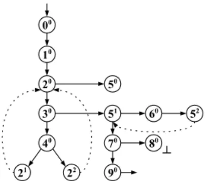
10 20 00 30 51 60 40 50 21 22 52 70 90 80 ┴
Figure 5: A partial unfolding of the LTS of Figure 4. remains: top (C 70) has been abstracted to a satisfiable
configuration and is thus unmarked.
70 is now visited, and its successors 80 and 90 are
built. The configuration of 80requires ib to be both lesser
and greater or equal to lb: 80 is marked (denoted by a
⊥ symbol in Figure 5).
Refine the faulty abstraction: 90 is reached. Since it
is an occurrence of the final location, we check if the unique4 path p in R from the red root to 90 is really
feasible, or if it has been made feasible by a previous abstraction.
Here p has been made feasible by the abstraction at 51.
A refine-and-restart phase is triggered. We extract from p the subpath p0 starting at 51 and ending after the first
infeasible step, namely 51· 70. We compute the weakest
precondition of false along p0, ia < la, and use it as the
limiting condition for abstraction at 51. Then, 51 has its
configuration before the abstraction restored, its subtree destroyed and 51 is finally pushed back on top of the
stack, and selected during the next iteration of build. Restart the analysis: The analysis restarts at 51, now
labeled with ia < la (denoted between square brackets in Figure 6). Its successors 61and 71are built and pushed
on the stack. Once again, the occurrence of 7 is detected infeasible and marked. The algorithm continues until 53
is processed. As previously, 53 is not subsumed by 51
since ia < la might not hold at 53. The algorithm
at-tempts at abstracting 51in order to force the subsumption
with 53 but now fails since the required abstraction does
not entail Φ(51) = ia < la.
End of the analysis: We do not detail the rest of the analysis as much. From 53, the second loop is unfolded
4Ris a tree and there is a unique path from the root to any vertex.
Taking into account the subsumption links could give an infinite number of paths and introduce more approximation.
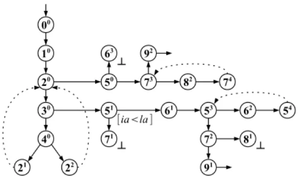
[ia<la ] 10 20 00 30 51 61 40 50 73 82 92 21 22 53 74 72 91 62 54 81 63 ┴ ┴ 71 ┴
Figure 6: A complete unfolding of the LTS of Figure 4. once again, reaching 54. Similarly to 53, the subsumption
(54, 51) cannot be established, since it would require to
abstract top (C 51) to the point where it does not entail
Φ(51)anymore. However, 54 is subsumed by 53 without
requiring any abstraction: none of their configurations require ia to be lesser than la anymore.
An occurrence of the final location is reached at 91
without asking for a refinement, since the two abstrac-tions made at 20 did not introduce any infeasible paths.
The first occurrence of 5, 50, is finally processed and
its subtree is completely built. The subsumption (74, 73)
needed to stop unfolding the third loop does not require an abstraction of 73: no refinement is needed when 92
is reached.
Interpretation of results: Once the analysis is over, the new LTS is obtained from the unfolding, as described in Section III. Let us call S0 this LTS (cf Figure 6). The
two following groups of infeasible paths of the LTS in Figure 4 have been eliminated in S0:
• paths going through both ending loops,
• paths exiting of the first loop through 3 ib≥ib→ 5
without going at least once through the second loop. However, S0 still contains five groups of infeasible
paths. We now show how the algorithm can be slightly modified to eliminate the remaining infeasible paths. B. Merging sort with feasible path sets comparisons
Recall that subsumption was defined as an inclusion of sets of program states represented by configurations. Hence, when the algorithm detects the subsumption of a red vertex by another, it is usually the case that the set of feasible paths going through the subsumee is a strict subset of the set of feasible paths going through the subsumer. Thus, adding such a subsumption introduces infeasible paths into the new graph. However, this is the price to pay in order to turn the potentially infinite symbolic execution tree into a finite graph.
The choice of the potential subsumer when trying to establish a subsumption is crucial for limiting the unfolding of loops without introducing too many infea-sible paths. The previous example shows that the first subsumption that can be established is not always (and often not) the best one in terms of pruning infeasible paths. We also observe that the refine-and-restart mech-anism can help us detect infeasible paths only when it is the shortest path to a given final red vertex that has been made feasible by some abstraction. We need additional mechanisms to control subsumptions to better detect infeasible paths.
An ideal definition of subsumption would require sets of feasible paths going through the two considered red vertices to be equal, but this is not realistic: this would require the full enumeration of paths starting at the two vertices, something very costly at best, and impossible when the sets are infinite. However, we can compare these sets of feasible paths starting at the two vertices up to a certain lookahead. Here we make the assumption that, given two red vertices representing the same original black location, the closer their sets of feasible paths, the lesser one will have to abstract the subsumer - if abstraction is needed at all - and the lesser infeasible paths are introduced into the new graph. To add this feature to the algorithm as shown in section III, one would have to surround the two If-Then blocks going from line 23 to 30 (Figure 3) by a third one, whose con-dition would be cmp_fp_sets(rv, rv0,
B, R, C) where cmp_fp_sets is responsible for comparing the two sets of feasible paths.
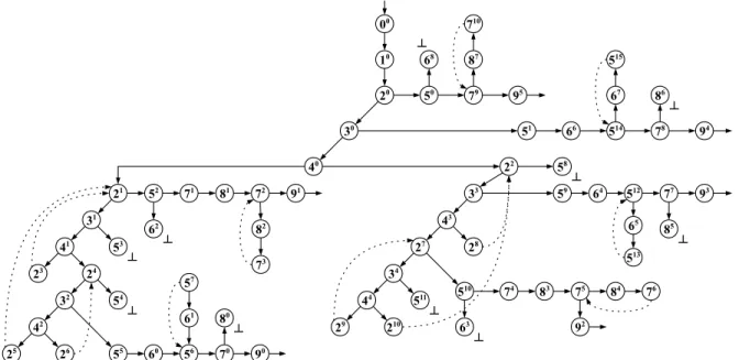
Applying the new algorithm in the previous context while comparing feasible paths sets up to a lookahead of two edges gives the complete unfolding shown in Figure 7, which contains no infeasible paths. In this example, no refine-and-restart phase is triggered for ob-taining this new LTS. Whenever the algorithm attempts at subsuming two occurrences of black vertex 2, com-paring sets of feasible paths starting at both occurrences up to a depth of two suffices to deduce which index was incremented last in the main loop and to decide if the subsumption will be precise enough. Also, when attempting to subsume occurrences of 5 (resp. 7), this lookahead mechanism prevents the abstraction to forget that ia (resp. ib) is lesser than la (resp. lb).
V. RESULTS
We now present experimental results obtained with our prototype when approximating the sets of feasible paths of three programs: merging sort, bubble sort and
00 10 20 30 40 21 31 41 24 32 42 55 60 56 61 70 90 71 81 72 82 52 22 51 66 514 67 78 79 87 50 33 43 27 34 44 510 74 83 75 84 59 64 512 65 77 93 91 92 94 95 23 25 57 26 73 29 210 28 76 513 710 515 53 54 80 62 511 58 85 68 86 ┴ ┴ ┴ ┴ ┴ ┴ 63 ┴ ┴ ┴ ┴
Figure 7: A complete unfolding of the LTS of Figure 4. No infeasible paths remain. substring search. These examples are simple but they all
have at least two unbounded loops with dependencies between the loops. The code of these programs are given in appendix. Merging sort has three successive loops; the inner loop in bubble sort is always executed the same number of times for each traversal of the outer loop; substring search has two nested loops related by a different kind of dependency.
For each of these programs, we first build new LTSs using different values of the current parameters of our tool: the way abstractions are computed, the depth of the lookahead and the fact that restarts are allowed or not. Then, for each LTS we compare the number of paths from the entry point to the exit of a given maximal length lwith the corresponding number of feasible paths. Paths are counted and drawn using the Rukia library [1]. Given an LTS S with n paths of length at most l, we draw uniformly at random n distinct paths of length at most l, then count the number of feasible paths. As the original and transformed LTS have the same set of feasible paths, counting feasible paths is more efficiently done in the new LTS that has a much smaller total number of paths. The second column of the tables shows which method for finding abstraction is used: with a = 1, abstractions are computed as shown in Section III; with a = 2, abstraction associates fresh symbolic values to program variables defined between the two candidates for
sub-sumption, until the subsumption is stated5.
A mark in the third column indicates if restarts are enabled for the experiment. Next columns give the number of paths of length at most l (eliminated paths are all infeasible) and the number of such feasible paths. A. Merging Sort
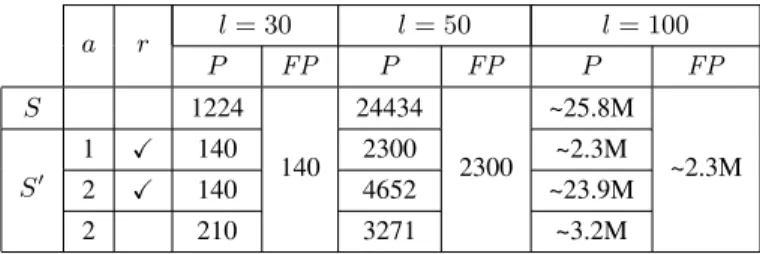
Table I shows the results for merging sort using a lookahead of two. The first line gives the results for the original LTS S from Figure 4. The second line shows the results for the LTS S0 built from the red-black graph
in Figure 7: no infeasible paths remain with the first method for finding abstractions.
When using the second method of abstraction and allowing restarts, the analysis does not terminate without bounding the length of paths. For merging sort, the ab-stractions computed this way are too crude to not trigger a restart. As said in Section III, since our algorithm does not learn yet from safeguard conditions, restart phases postpone subsumptions, but the same phenomenon can occur again after unfolding the loop. Learning from the safeguard-condition when computing abstractions would rule out such chains of restarts.
The third line gives the results obtained with the second method of abstraction, mrl being set to 30. The red part is no longer complete, and the LTS in which paths are drawn is obtained by connecting the
5Abstracting configurations in this way requires to combine them
Table I:Paths (P ) and feasible paths (FP) in merging sort. a r l = 30 l = 50 l = 100 P FP P FP P FP S 1224 140 24434 2300 ~25.8M ~2.3M S0 1 X 140 2300 ~2.3M 2 X 140 4652 ~23.9M 2 210 3271 ~3.2M
red vertices that were not expanded to the black part. A path of length at most 30 is entirely in the red part. Paths of length more than 30 can end in the black part rather than in the red one.
The fourth line shows the results for the LTS obtained with the second method of abstraction, disabling restarts. Without restarts, the second method of abstraction de-tects a fair number of infeasible paths.
B. Bubble Sort
Table II gives the results for bubble sort6. With a
lookahead of 0 or 1 and either method of abstraction, the only infeasible path removed is the one that does not enter the outer loop. With a lookahead of at least 2, S0 better approximates the set of feasible paths: from
2 to 7, the algorithm produces the same LTSs, but at 8, more dependencies about traversals of the inner loop are discovered. The value of the lookahead cannot be increased too much in practice as comparing the sets of feasible paths of candidates is exponential.
Method of abstraction 1 performs worst here. In bub-ble sort, a variabub-ble keeps track whether any permutation occurs during a traversal of the inner loop. Information about the value of this variable can be lost when ab-stracting the configuration at the entry of the inner loop, introducing infeasible paths. This phenomenon does not happen with method 2.
With both methods, the analysis terminates without the need of mrl. There remains a fair number of infeasible paths in S0. Unlike merging sort, the set of feasible paths
of bubble sort is not a regular language because of the dependency between the number of traversal of its two loops. We believe that the results in Table II can be improved with more accurate methods of abstraction, but bubble sort clearly shows some limitations of our approach in its current state.
C. Substring
Table III shows the results for substring. The function takes as input strings s1 and s2, and returns true if s2 is
6Discriminating feasible paths for l = 100 was not tractable here.
Table II:Paths and feasible paths in bubble sort. An additional column gives the depth for the lookahead.
a r la l = 30 l = 50 l = 100 P FP P FP P S 1474 20 643692 217 ~2.3 × 10¹² S0 1 X 2 741 321962 ~1.2 × 10¹² 2 X 203 44504 ~2.9 × 10¹¹ 1 X 8 285 69457 ~6.6 × 10¹⁰ 2 X 10³ 13249 ~6.4 × 10⁹
Table III: Paths and feasible paths in substring.
a r la l = 30 l = 50 l = 100 P FP P FP P S 1433 87 195874 2108 ~4.2 × 10¹⁰ S0 1 X 0 143 4180 9227464 2 X 1 X 10 130 3803 8395424 2 X 98 2818 6217117
a substring of s1. Loops present some dependencies: for
example, let s be a (strict) prefix of s2of length lsfound
to be a substring of s1. Then s2 has length at least ls,
and no latter iteration of the outer loop can return true without doing at least lscomparisons. The set of feasible
paths of substring is not a regular language.
With a lookahead of 0, both methods of abstraction produces the same LTS: the path that returns false when s2 is empty is ruled out, and the algorithm discovers the
above property for ls= 1. New LTSs are produced with
a lookahead of 10: the algorithm now (re-)discovers the property for ls= 1 and ls= 2.
Again, the analysis terminates without bounding mrl. VI. AFORMAL THEORY FOR THE GRAPH
TRANSFORMATIONS
In [6] we present a formal model for our notion of con-figurations and for the graph transformations on which our prototype is based. The model makes a conceptual split between the fundamental aspects (symbolic evalua-tion, abstracevalua-tion, subsumptions, predicates for limiting abstraction) and the heuristics parts of the algorithm (restricting abstractions and subsumptions). A model of the CFG (as a labeled transition system), paths, configu-rations is developed in Isabelle/HOL [11] and a calculus is provided in which each graph transformation is defined as either a partial unfolding of the CFG (symbolic execu-tion, subsumption arc linking vertices) or an annotation associated with a vertex (abstraction represented by a
weakening of the path predicate, limitation of possible abstraction by additional formulae, marking vertices as unsatisfiable). The two key properties of Section III have been proved, namely: the preservation of traces along the paths of the original CFG and the preservation of feasible paths.
Our prototype has the same conceptual organization, with concrete heuristics for restricting abstractions and subsumptions added on top of the basic graph trans-formations. Although we did not develop the entire system within the model, the formal proofs give strong confidence of the correctness of the implementation.
VII. RELATED WORK
Unfeasible paths are a general problem when testing programs or checking models. There is an abundant literature that is not reviewed here due to lack of space, where symbolic execution is widely exploited. For a re-cent account of issues in this area we refer to [3, 12, 13]. A notable advance is concolic testing [14, 15] where actual execution of the program under test is coupled with symbolic execution. It reduces the detection of infeasible paths to those paths that go one branch further than some feasible one, alleviating the load of the con-straint solver and decreasing significantly the number of paths to be considered. This approach leads to coverage of all feasible paths. Some randomness can be introduced in the choice of the next branch to be examined, as mentioned in [15], but the resulting distribution on paths suffers from the drawback of isotropic random walks, yielding unbalanced coverage of paths.
To ensure uniform random coverage of paths (and more generally a maximum minimal probability of cov-ering components of a coverage criterion [1]), a global knowledge of the graph is required. Thus concolic or similar dynamic approaches cannot be used: some global static analysis is required. It is the application scenario that motivated the work presented here.
We have taken inspiration from [9] and [16], where subsumptions, abstractions and interpolation are used to verify unreachability of selected error locations. Here, the problem we address is to preserve feasibility rather than infeasibility. This requires specific finer strate-gies for subsumptions and abstractions: reusing the ap-proaches of [9] and [16] would lead to graphs polluted by numerous new infeasible paths.
The problem of unbounded loops is a general issue for methods based on symbolic execution [10, 17]. It is generally treated, as we do, by searching for subsump-tions, which doesn’t always terminates. The red-black
graph data structure we have defined makes it possible to deal with these non terminating cases.
Other potential application scenarios of the graph transformation proposed here include paths selection for satisfying coverage criteria of elements of a graph, for instance branches [13], or mutation points [18].
VIII. CONCLUSION
In this work we address the problem of graph trans-formations that discard infeasible paths, preserving the behaviour of the program, with path-biased random testing in mind.
The size of the resulting graph and the length of paths are not a problem for drawing since the Rukia library we use for drawing paths scales up extremely well [1]. We expect the time of construction of the transformed graph to remain reasonable, thank to the progresses of symbolic execution tools and constraint solvers. The first results are encouraging since, on the current examples, the cost of this preprocessing phase is not an issue, and quite a significant number of infeasible paths are discarded, even with a basic set of heuristics.
We plan various improvements of the prototype aim-ing at improvaim-ing the quality of the result, i.e. the pro-portions of infeasible paths in the transformed graph. We investigate better control of abstractions, taking advan-tage of safeguard conditions and interpolant propagations in the spirit of [10]. Using existing methods based on abstract interpretation and dataflow analysis [19, 20] will help finding abstractions by providing ranges of values for some variables, i.e. some kind of additional invari-ants. Besides, we plan to extend the range of application of our approach by integration of memory models and additional language constructs. Our method could also be improved by using generalisation of infeasible paths as proposed in [21] for concolic testing.
REFERENCES
[1] A. Denise, M.-C. Gaudel, S.-D. Gouraud, R. Lassaigne, J. Oudinet, and S. Peyronnet, “Coverage-biased random explo-ration of large models and application to testing,” STTT, vol. 14, no. 1, pp. 73–93, 2011.
[2] P. Thévenod-Fosse and H. Waeselynck, “An investigation of statistical software testing,” Softw. Test., Verif. Reliab., vol. 1, no. 2, pp. 5–25, 1991.
[3] C. Cadar and K. Sen, “Symbolic execution for software testing: three decades later,” CACM, vol. 56, pp. 82–90, 2013. [4] S. C. Ntafos, “On comparisons of random, partition, and
pro-portional partition testing,” IEEE Trans. on Soft. Eng., vol. 27, no. 10, pp. 949–960, 2001.
[5] S.-D. Gouraud, “Utilisation des structures combinatoires pour le test statistique,” Ph.D. dissertation, Université Paris-Sud 11, LRI, 2004.
[6] R. Aissat, F. Voisin, and B. Wolff, “Infeasible paths elimina-tion by symbolic execuelimina-tion techniques: proof of correctness and preservation of paths,” in ITP’16, ser. LNCS, vol. 9807. Springer, 2016.
[7] M. Trtík and J. Strejˇcek, “Symbolic memory with pointers,” in Automated Technology for Verification and Analysis - 12th International Symposium, ATVA 2014, Sydney. Springer, 2014, pp. 380–395.
[8] F. Besson, S. Blazy, and P. Wilke, “A Precise and Abstract Memory Model for C Using Symbolic Values,” in 12th Asian Symposium on Programming Languages and Systems, Singa-pore, ser. LNCS, vol. 8858. Springer, 2014, pp. 449 – 468. [9] T. A. Henzinger, R. Jhala, R. Majumdar, and K. L. McMillan,
“Abstractions from proofs,” in POPL’04. ACM, 2004, pp. 232–244.
[10] K. L. McMillan, “Lazy annotation for program testing and verification,” in CAV’2010, ser. LNCS, vol. 6174. Springer, 2010, pp. 104–118.
[11] T. Nipkow, L. C. Paulson, and M. Wenzel, Isabelle/HOL—A Proof Assistant for Higher-Order Logic. Springer-Verlag, 2002. [12] S. Bardin, M. Delahaye, R. David, N. Kosmatov, M. Papadakis, Y. L. Traon, and J. Marion, “Sound and quasi-complete detec-tion of infeasible test requirements,” in 8th ICST. IEEE, 2015, pp. 1–10.
[13] M. Papadakis and N. Malevris, “A symbolic execution tool based on the elimination of infeasible paths,” in The Fifth Inter-national Conference on Software Engineering Advances, ICSEA 2010, 22-27 August 2010, Nice, France. IEEE Computer Society, 2010, pp. 435–440.
[14] N. Williams, B. Marre, P. Mouy, and M. Roger, “Pathcrawler: Automatic generation of path tests by combining static and dynamic analysis,” in EDCC-5, ser. LNCS, vol. 3463. Springer, 2005, pp. 281–292.
[15] J. Burnim and K. Sen, “Heuristics for scalable dynamic test generation,” in ASE’2008. IEEE, 2008, pp. 443–446. [16] J. Jaffar, V. Murali, J. A. Navas, and A. E. Santosa, “TRACER:
A symbolic execution tool for verification,” in CAV 2012, ser. LNCS, vol. 7358. Springer, 2012, pp. 758–766.
[17] J. Jaffar, J. A. Navas, and A. E. Santosa, “Unbounded symbolic execution for program verification,” in RV’11, ser. LNCS, vol. 7358. Springer, 2011, pp. 396–411.
[18] M. Papadakis and N. Malevris, “Mutation based test case gen-eration via a path selection strategy,” Information & Software Technology, vol. 54, no. 9, pp. 915–932, 2012.
[19] R. Bodík, R. Gupta, and M. L. Soffa, “Refining data flow information using infeasible paths,” in Proceedings of the 6th European SOFTWARE ENGINEERING Conference Held Jointly with the 5th ACM SIGSOFT International Symposium on Foundations of Software Engineering, ser. ESEC ’97/FSE-5. New York, NY, USA: Springer-Verlag New York, Inc., 1997, pp. 361–377.
[20] V. Raychev, M. Musuvathi, and T. Mytkowicz, “Paralleliz-ing user-defined aggregations us“Paralleliz-ing symbolic execution,” in Proceedings of the 25th Symposium on Operating Systems Principles, ser. SOSP ’15. New York, NY, USA: ACM, 2015, pp. 153–167.
[21] M. Delahaye, B. Botella, and A. Gotlieb, “Infeasible path generalization in dynamic symbolic execution,” Information & Software Technology, vol. 58, pp. 403–418, 2015.
IX. APPENDIX
void merge (int ∗ a, int la , int ∗ b, int lb , int ∗ A){ ia := 0; ib := 0; while ( ia < la && ib < lb){ if (a[ ia ] < b[ib]){ A[ia+ib] := a[ ia ]; ia := ia + 1; } else { A[ia+ib] := b[ib ]; ib := ib+1; } } while ( ia < la){ A[ia+ib] := a[ ia ]; ia := ia + 1; } while ( ib < lb){ A[ia+ib] := b[ib ]; ib := ib + 1; } }
void bubble (int ∗ a, int l){ int i , swapped = 1, tmp; while (swapped != 0){ swapped = 0; i = 1; while ( i < l){ if (a[ i −1] > a[i]){ tmp = a[i ]; a[ i ] = a[i−1]; a[ i−1] = tmp; swapped = 1; } i ++; } } }
int factor (char ∗ s1, int l1 , char ∗ s2, int l2){ int i = 0, j ; while ( i <= l1 − l2){ j = 0; while ( j != l2){ if (s2[ j ] == s1[i+j]){ j++; } else break; } if ( j == l2) return 1; i ++; } return 0; }