The Stability and Growth Pact will lead member countries to aim for cyclically balanced budgets. Until this steady state is reached, Europe will continue its efforts at deficit cutting. While so doing, politicians are less likely to undertake the difficult labour market reforms that are really needed. Is further fiscal retrenchment wise? The paper reviews the reasons that have been advanced in favour of a Stability Pact and finds them wanting. The most serious justifications, such as the systemic risk of bank crisis following a government’s failure to service its debt, can be better dealt with in other ways: for example, by prudential limits on banks’ exposure to public debts. Moreover, our analysis reveals that the macroeconomic costs of the Stability Pact, while sizeable, are not as dangerous as often believed. The costs will be barely visible once the steady state is reached. The true macroeconomic costs are front loaded; they concern the next few years, after a decade already dominated by convergence efforts.
— Barry Eichengreen and Charles Wyplosz
More than a minor nuisance?
SUMMARY
Economic Policy April 1998 Printed in Great Britain © CEPR, CES, MSH, 1998.
1. INTRODUCTION
The Maastricht Treaty provides the institutional framework for Europe’s monetary union. Its essential features have been the subject of extensive discussion: these include the three-step transition, the creation of a European Central Bank, procedures for shaping the conduct of fiscal policy (the Excessive Deficit and Mutual Surveillance Procedures of Art. 103, 104 and 109) and the no-bailout rule prohibiting the ECB from acquiring public debt directly from the issuer (Art. 104 of the treaty and Art. 21 of the Protocol on the European System of Central Banks).
The one post-Maastricht element, finalized at the June 1997 meeting of the European Council in Amsterdam, is the Pact for Stability and Growth.1 The pact clarifies the provisions of the Excessive Deficit Procedure. It calls for fiscal
The Stability Pact:
more than a minor nuisance?
Barry Eichengreen and Charles Wyplosz
IMF, University of California, Berkeley, CEPR and NBER; Graduate Institute of International Studies, Geneva, and CEPR
For help with data we thank Tamim Bayoumi, Herve Daudin, Paul De Grauwe, Tom Fernley, Morris Goldstein, Patrick Honohan, Alessandro Missale, Th. Papaspyrou, Ole Marius Tideman, Giuseppe Tullio, Bill White and Geoffrey Woglom. Xavier Debrun, Arjan Kadareja, Darren Lubotsky and Matthew Olson provided efficient research assistance. Financial support was provided by FNRS in Switzerland and the Center for German and European Studies of the University of California as well as the National Science Foundation in the United States. The opinions expressed are not necessarily those of the International Monetary Fund. Without implicating them in our conclusions, for helpful comments and guidance we would like to thank Donogh McDonald, the members of the Economic Policy Panel, our discussants, the journal’s referees and David Begg.
1
The ‘growth’ part was added at the request of the French authorities as a face-saving device after they were forced to soften their previous opposition.
positions to be balanced or in surplus in normal times so that automatic stabilizers can operate. It urges stronger surveillance of medium-term fiscal positions with the goal of providing an early warning signal that the 3% reference value for budget deficits is at risk. It clarifies the conditions under which participants in the monetary union will be allowed to exceed the 3% deficit ceiling without being determined to have an excessive deficit. Countries will be automatically exempt only if their GDPs have declined by 2% and the excess deficit is temporary and small. Those in which GDP declines by between 0.75% and 2% could also be exempt, but only with the concurrence of the Council of Ministers. Countries with even milder recessions will be found to have an excessive deficit and forced to make mandatory deposits that are transformed into fines if the fiscal excess is not eliminated within two years.
Although this new transparency is welcome, it also reveals a more restrictive set of provisions than those laid down by the Maastricht Treaty. The treaty says only that the general government deficit may not exceed its reference value (3% of GDP) unless the deficit has declined significantly and continuously to where it is close to that reference value, or the excess of the reference value is only exceptional and temporary and the deficit remains close to the reference value. It says nothing, in other words, about the size of the output decline producing that exceptional and temporary excess deficit, or the period over which it must occur. In this sense the Stability Pact implies less flexibility than the Maastricht Treaty.
The Stability Pact has not received the same systematic analysis as other aspects of the Maastricht Treaty.2 Providing that analysis is our purpose in this paper.
Our conclusion is that the Stability Pact will have some effect. Governments will adjust their fiscal policies just enough to avoid incurring fines. EU authorities for their part will give countries just enough leeway to avoid having to fine them. Actually imposing fines would worsen conditions in the adversely affected member state, lead to recrimination and deal a blow to EU solidarity. Actually incurring fines would subject a government to serious embarrassment and loss of political face. Hence, the pact is likely to alter fiscal behaviour just enough to avoid these outcomes.
This will reduce the extent of automatic stabilization. Estimates based on historical data suggest that automatic stabilization may increase in the output gap, but by only a fraction of a percentage point. Hence the ‘minor nuisance’ of the title. But even a fraction of a percentage point on the growth rate can become important when allowed to accumulate over time. Our simulations suggest that, after accumulation over the last two decades, levels of real output would have ended 5% lower in France and the UK, and 9% lower in Italy.
The critical question, therefore, is how hamstrung automatic stabilizers will be. Will the Stability Pact weaken them as much in the future as it would have in the past, had it been superimposed on actual experience? The answer hinges on how far below the 3% ceiling budget deficits are when Stage III begins. If budgets move significantly into surplus relative to past experience, there is no reason why automatic stabilizers will be much affected. But in the present climate, where electorates lack the appetite for further spending cuts, significantly smaller deficits require significantly faster growth. The danger is thus that the Stability Pact will divert effort from the fundamental reforms needed to step up the pace. In particular, without fundamental labour market reform, Europe will fail to grow by at least 3 – 31_
2% a year, and deficits will not decline. The Stability Pact will grow more binding, and the operation of Europe’s automatic stabilizers will remain feeble, increasing the volatility of output, further depressing growth, and making the provisions of the pact even more binding than before. Through the operation of this vicious spiral, Europe could be condemned to a low-level equilibrium trap.
Our view is that leaders have a fixed amount of political capital that they can allocate to politically costly fiscal reform or politically costly labour market reform. To the extent that they invest in one, they have fewer resources left to devote to the other. In practice, they are likely to compromise, doing a little of each. For example, those European countries that have made the most progress in eliminating budget deficits and increasing labour market flexibility (Ireland and Finland spring to mind) have allocated their adjustment effort evenly to fiscal consolidation and labour market reform.
Our conclusion will be that the Stability Pact may have some slight benefits in terms of fiscal discipline, but may have significant costs, both in diverting political effort from more fundamental problems and indeed in making those fundamental problems worse than before.
2. WHAT THE STABILITY PACT SAYS
The Stability Pact consists of two Council regulations, one on the Excessive Deficit Procedure and another on surveillance, and a European Council resolution that provides guidance to the Council and member states on the application of the pact. The two Council regulations have the force of law. They clarify the meaning of the Maastricht Treaty’s provisions regarding excessive deficits, in particular in respect of exceptional and temporary circumstances under which the 3% reference value for the general government deficit can be exceeded without a determination that the deficit is excessive. In addition, under the pact’s provisions, participants in the monetary union commit themselves to a medium-term budgetary stance ‘close to balance or surplus’.
The pact will consider a deficit in excess of 3% to be exceptional if a country’s GDP declines by at least 2% in the year in question. In addition, a recession in which real GDP declines by less than 2% but more than 0.75% may qualify with the concurrence of the Council. The country will have to show that its recession was exceptional in terms of its abruptness or in relation to past output trends. Countries with annual output declines smaller than 0.75% will not be able to claim exceptional circumstances. These provisions thus clarify the Maastricht Treaty’s clauses regarding the exceptional circumstances under which the 3% reference value can be exceeded without leading to the determination of an excessive deficit.
The pact also includes provisions concerning further exemptions. While countries are obliged to correct excessive deficits ‘as quickly as possible after their emergence’ and to ‘launch the corrective budgetary adjustments they deem necessary without delay’, they will probably be able to run deficits in excess of 3% of GDP for at least two years in a row without incurring fines. The Commission will receive definitive data that a country’s deficit in year t exceeded 3% around March of year t + 1. By the end of May it will have issued a recommendation for eliminating that excess in accordance with Article 103(4). The country will then have to take corrective action such that the excess is eliminated by year t + 2. If no corrective action is taken by the end of year t + 1, financial sanctions will be imposed. But presumably corrective action that will eliminate the excess in year t + 2 will suffice to eliminate this threat. Thus, two successive years of budget deficits in excess of 3% (and possibly more – see below) will be permitted.
Moreover, the passage specifying these time limits ends with the qualifying phrase ‘unless there are special circumstances’. The nature of those special circumstances is not specified. But presumably a country like Finland in the early 1990s, which suffered budgetary difficulties reflecting special circumstances largely beyond its control, would be allowed to take even longer to bring its deficit back down to 3%. Nor does the pact clarify a third provision of the Excessive Deficit Procedure, that the budget must remain ‘close’ to the reference value to avoid the determination of an excessive deficit.
Sanctions, when required, will take the form of non-remunerated deposits, which start at 0.2% of GDP and rise by one-tenth of the excess deficit up to a maximum of 0.5% of GDP. Additional deposits will be required each year until the excessive deficit is corrected. If the excess is not corrected within two years, the deposit will be converted into a fine; otherwise it will be returned.
Thus, a careful reading does not imply that fines will be levied as soon as budget deficits exceed 3% of GDP. The pact is rather more flexible. It allows temporary exemptions for countries experiencing ‘severe’ recessions. More generally, it allows time for excessive deficits to be corrected; in the case of undefined ‘special circumstances’ it allows unspecified amounts of time. Clearly, one needs to think harder about the political economy of EU policy making to forecast how strictly the fines and sanctions of the Stability Pact will be applied.
3. RATIONALES FOR THE STABILITY PACT
For an argument favouring the Stability Pact to convince, it must satisfy three conditions. The effect on which it hinges must be first order (on the principle that controversial policies with potentially important side-effects should not be adopted in response to negligible problems). It must have Europe-wide repercussions (on the principle that, if its effects are purely national, there is no justification for a Europe-wide response). And, arguably, it must be a consequence of monetary union rather than a corollary of European integration (on the principle that the Excessive Deficit Procedure and the rest of the Maastricht Treaty apply to member states whether in or out of the monetary union, whereas the sanctions of the Stability Pact apply specifically to participants in EMU).3
3.1. To prevent inflationary debt bailouts
The most compelling argument for the Stability Pact is as extra protection for the ECB from pressure for an inflationary debt bailout. The scenario might run as follows. The government of an EMU country gets into fiscal trouble, from which it cannot extricate itself. Investors fear suspension or (more likely) modification of payment on its public debt , and therefore sell its bonds. Its bond prices start to plummet. Banks holding those bonds find their capital impaired, inciting depositor runs. Bond markets (and indirectly banks) in other EMU countries suffer adverse repercussions, as investors in public debt of other European states become demoralized. To prevent the collapse of Europe’s banking and financial system, the ECB buys up the bonds of the government in distress. As the costs are being borne by the residents of the EMU zone as a whole rather than the citizens of the responsible country, governments have an incentive to run riskier policies in the first place, and investors have less reason to apply market discipline.
This scenario is more than hypothetical: in 1994 – 5 something similar occurred in Mexico (see Box 1). But is it relevant to Europe? Recent debt problems, not just in Mexico but in Thailand, South Korea and elsewhere, suggest that the monetary authorities (the ECB in Europe, the IMF in the broader international context) come under intense pressure to extend a debt bailout when two conditions hold: debt problems place the banking system at risk; and they threaten to spread contagiously to other national markets.4 Banks are the weak link in the chain of macroeconomic and financial stability: their core business, maturity transformation, renders them
3
The point is arguable because other pact provisions, such as medium-term surveillance and the precise conditions under which a deficit will be found as excessive, will apply to EU countries whether or not in EMU.
4
The probability of bailouts is further enhanced by serious imbalances in the vertical structure of taxation and spending, when the centre collects the taxes but subcentral governments receive transfers and do the spending. This works against the likelihood of a debt bailout in Europe, where member states collect the bulk of their own taxes, and where transfers from the EU remain relatively small. We develop these points further in Box 2.
illiquid. Operating in an environment of asymmetric information, they are vulnerable to runs when depositors lack confidence. The Great Depression reminds us that widespread bank failures can have serious macroeconomic repercussions. Contagion provides major motivation for IMF intervention in countries like
Box 1. Should Stability Pact proponents fear that Europe will be another Mexico?
A precedent for the bailout scenario feared by European policy-makers is the Mexican crisis of 1994 – 5 (for an overview and analysis on which we draw, see Sachs et al., 1995). That episode points to four factors that magnify bailout risk. First, a significant share of Mexican public debt, the notorious tesobonos, was foreign-currency indexed. Since the Bank of Mexico could not print dollars and was committed to holding the exchange rate within a band, once investors began selling its bonds, the Mexican government was in the same predicament as a member of a monetary union. It could purchase what was being sold only in so far as it possessed dollar reserves. Since its reserves were limited, it had to solicit a bailout from the USA and the IMF.
Second, much of Mexico’s debt was short term. The tesobonos and their domestic-currency equivalents, cetes, ran only 30, 60 or 90 days to maturity. Not only did the government have to service its debts, but it had to redeem a significant quantity if investors failed to roll them over. Since it lacked the dollars to do so and might print pesos to finance redemptions, the spectre of inflation loomed. Doubts about the government’s willingness or ability to service its debts could therefore ignite a run.
Third, significant quantities of public debt were held by the Mexican banking system, whose stability was critical for the macroeconomy. The outbreak of the crisis was followed immediately by withdrawals by domestic and foreign depositors. Fear of collapse of the banking system was a powerful motive for the rescue by the USA and IMF.
Fourth, there were fears of contagion. The Mexican crisis led to extensive reserve losses and deposit withdrawals in Argentina and repercussions as far afield as Thailand, Hong Kong and Sweden. US officials cited danger of contagion and systemic risk as a rationale for the Mexican bailout.
Each of these points has an analogy in EMU. National central banks will be mere operating arms of the ECB, unable to print euros. Some candidates for EMU have significant amounts of short-term debt, held in important part by the banking system. And as European banking systems and financial markets more generally become increasingly integrated and interdependent, worries of contagion will grow.
Box 2. Sooner or later? When will bailout risk be greatest?
At what stage in the construction of EMU will bailout risk be greatest? McKinnon (1996) suggests it will be most intense at the start; von Hagen and Eichengreen (1996) argue that bailout risk will be least at the outset.
McKinnon’s conclusion follows from assuming that bailout risk is minimized when four conditions are met:
monetary separation (the government neither owns nor controls the central bank). Monetary separation hardens budget constraints, discouraging governments from recklessly accumulating debts.
fiscal separation (little co-mingling of revenues of different levels of government, so lower levels of government cannot expect additional transfers from higher levels when they overspend). When lower levels of government receive transfers, their budget constraints are softened, and they may be tempted to run reckless fiscal policies.
factor mobility, intensifying tax competition and limiting the size of the public
sector. This, in McKinnon’s view, will limit the size of the public sector debts that member states accumulate.5
low debt/GNP ratios, so that governments do not pressurize the monetary authorities to use the inflation tax on optimal-taxation grounds.6
The first three conditions will be met from the outset. The single market, by encouraging factor mobility, will intensify tax competition. No national government will have its own central bank. Revenue sharing will be minimal. If there is bailout risk, it will arise from failure to meet the final condition, a failure that will be most egregious in the short run. This implies that the need for the Stability Pact is most pressing in the early years of EMU but less so subsequently (when debt overhangs have been removed).
Von Hagen and Eichengreen emphasize that bailout risk will depend on the vertical structure of the tax base: in other words, on the extent to which subcentral – in the context of EMU, member state – governments collect their own taxes versus relying on transfers from the centre. Contrast two situations. In scenario A, all taxes are raised by a central government that provides grants to subcentral governments. If a subcentral government experiences difficulties, its
Continued
5
The counterargument, which we regard as more plausible, is that tax competition will put downward pressure on revenues, but its impact on expenditure may be less than one for one. For this reason it may be associated with larger deficits and debts, not smaller ones.
6A clear analysis of how high debt burdens lead governments to press for use of the inflation tax in the Ramsey model is De Grauwe (1996).
Box 2. continued
only options are to default or obtain a bailout. If default is not politically palatable, then a bailout will be forthcoming. A subcentral government that knows this will have an incentive to run risky policies.
In scenario B, subcentral governments control their own taxes. If they experience difficulties, they can be asked to raise the tax rates they control, reinforcing their financial position. Since in this case there exists a lower-cost alternative to default, the central bank can credibly promise not to provide a bailout.7
It follows that pressure for a bailout will be intense in the early years of EMU. The European Union lacks a highly developed system of fiscal federalism. Its budget is small, and the vast majority is earmarked for the common agricultural policy and Structural Funds (leaving it unavailable for treating debt- and deficit-related problems). The member states control the taxes levied on their citizens. This will give national governments a third, low-cost, alternative to default and bailout: namely, adjusting their own tax rates to redress their own financial problems. The ECB, aware of the existence of this third alternative, should be able to resist the pressure for a bailout.
Eventually there may develop pressure for a European system of fiscal federalism to smooth the operation of the monetary union, in which case the vertical structure of the tax base will be transformed and with it the severity of bailout risk. But this is a long-run prospect. Thus, in contrast to McKinnon, who sees bailout risk as most intense in the short run, von Hagen and Eichengreen and the present authors see it as more pressing later.
Correctly choosing between these models is important, for erroneously accepting one could aggravate the very problems forecast by the other. Say that one accepts McKinnon’s interpretation and adopts strict limits on fiscal policy. If member states are then prevented from operating their automatic fiscal stabilizers in response to business-cycle disturbances, they will press the EU to do so for them. They will lobby for an expanded EU budget with automatic-stabilization capacity and transfers from the EU to the member states. Ultimately this could lead to precisely the bailout problem about which the proponents of the Stability Pact are so concerned.
7Von Hagen and Eichengreen test this hypothesis by estimating a probit regression on cross-country data for 1985 – 7. The presence or absence of fiscal restrictions on subcentral governments, which will be needed where bailout risk is most intense, is modelled as a function of the share of subcentral government spending financed out of own taxes. (Per-capita income is also included as a control.) The results confirm that the vertical structure of taxation matters for the incidence of fiscal restrictions and by implication for bailout risk.
Mexico, Thailand and South Korea; if a crisis in one country has major inter-national externalities that inter-national policy-makers have little incentive to internalize, there is an obvious argument for multilateral intervention (in the European case, by the ECB).
We take seriously the rationale for the Stability Pact based on the spectre of an inflationary debt bailout. But the Maastricht Treaty already contains a no-bailout rule that prohibits the ECB from purchasing public debt directly from the issuer. To justify reinforcing this rule with a Stability Pact, it is necessary to show that the factors heightening bailout risk – threats to the banking system and bond market contagion – will operate in EMU: in other words, that the risks to Europe’s banking system and bond markets are sufficiently intense that the ECB will be unable to resist importuning by heavily indebted countries. We provide evidence on these questions below.
3.2. To neutralize inflationary pressure more generally
A second popular rationale for the Stability Pact is to offset other sources of inflationary pressure. The ECB, concerned to maximize economic efficiency, will seek to balance the deadweight cost of the inflation tax against the deadweight cost of other taxes. Where the total resources required by the public sector are large, all taxes, including the inflation tax, will be high. If governments of EMU countries run large deficits and accumulate high debts, the ECB will permit more inflationary monetary policies to reduce the deadweight losses associated with other taxes. Since product and factor market taxes fall on the residents of each country, while the inflation tax will be shifted to the residents of the whole euro zone, national incentives to run deficits will be increased by EMU membership.
This analysis, as in De Grauwe (1996), presupposes that the ECB will be simply a Stackelberg follower to the fiscal lead of different member governments. However, there are convincing reasons to think that the ECB will not act as a myopic follower of fiscal fashion, but will engage in a repeated game in which it seeks to convince governments and markets of the credibility of its commitment to price stability. It will keep inflation low even if this means that other taxes have to be higher.8 Governments, finding the deadweight loss of taxation to be higher, may then pursue lower government spending. They will be Stackelberg followers, not leaders.
Thus, there is good reason to think that any inflation bias in ECB policies produced on optimal taxation grounds will be small. This is a weak reed, hardly first order in magnitude, on which to rest any justification for the Stability Pact.
8If EMU members appoint independent central bankers who attach overriding importance to the goal of price stability, even a myopic ECB will be reluctant to trade off higher inflation tax revenue for reductions in distortions from other sources of tax revenue.
3.3. To offset political bias towards excessive deficits
A third widely voiced rationale for the Stability Pact is to offset Europe’s bias towards excessive deficits (Beetsma and Uhlig, 1997). Years of deficit spending have saddled governments with debt/GDP ratios in excess of 70%. High debts make the public finances more fragile, reduce the effectiveness of monetary policy (Giavazzi et
al., 1997), increase fiscal crowding out (since additional government spending, by
raising interest rates, thereby raises debt service costs), raise the deadweight cost of taxation, and make funding social security liabilities more difficult.
The solution is to move Europe’s budgets towards balance sufficiently to stabilize the debt/income ratio or to allow it to decline. Thus, the Stability Pact sees Europe’s budgets as broadly balanced or in modest surplus in expansions, with deficits widening to as much as 3% of GDP in contractions. With real GDP growing at 2 – 3% per year, this should suffice for debt/income ratios to fall over the medium run.
The obvious objection to this rationale for the Stability Pact is that it suppresses the symptoms without eradicating the disease. If EU policy-makers fail to remove the underlying disorder – identified by the ‘institutional school’9 as excessively decentralized fiscal procedures that aggravate free-rider problems – then imposing numerical caps on budget deficits only encourages devious behaviour to meet the letter but not the spirit of the law. We need only note the operation of the Excessive Deficit Procedure. While some progress has been made in curbing deficits in Stage II, the EDP has also encouraged fiscal fiddles like refundable ‘euro taxes’, sales of central bank gold reserves and one-off appropriations of public enterprise reserves. It remains to be seen how much recent progress is sustainable. Pessimists (including one of the authors) worry that, in the absence of an effective remedy for the underlying disorder, ‘Maastricht fatigue’ will set in once countries are admitted to EMU, as refundable euro taxes are refunded and, more generally, as countries previously forced to suck in their stomachs to squeeze into Maastricht’s tightly tailored trousers then expel their breath violently.10
However, suppressing the symptoms is standard practice when the disease is untreatable. Doctors administer powerful pain-killers to patients with untreatable cancers. If excessive deficits can be prevented only by using the EU’s authority to impose a credible external constraint, there is no reason not to try.
3.4. To internalize international interest rate spillovers
Another popular justification for the Stability Pact is to internalize the cross-border interest rate spillovers associated with uncoordinated fiscal policies. Policy-makers,
9
See Alesina and Perotti (1994), von Hagen and Harden (1994) and Alesina et al. (1995). 10See Eichengreen (1997).
in this view, have inadequate incentive to take into account the impact of their borrowing on interest rates in other member states when formulating their national fiscal policies. The Excessive Deficit Procedure and the Stability Pact offset this bias. However, European countries borrow in global not national financial markets: it is unclear how fiscal policy in Italy and Spain has significant effects on interest rates in Germany or France.
Even if they did, in the absence of other distortions, changes in interest rates are purely redistributive. They redistribute income from debtors to creditors, within and across EU states. Table 1 suggests that higher interest rates would mean redistribu-tion from the Nordic countries, Spain and Italy towards Germany and the Benelux countries. Ironically, core members of the future EMU should be the last countries to worry about redistributive effects of high interest rates! In any case, in so far as these externalities are pecuniary, they do not warrant intervention on standard efficiency grounds (Buiter et al., 1993).
Of course, in the presence of other distortions, such as rigid wages, changes in interest rates can have cross-border effects on the level of output and employment. But these are unlikely to be significant, not least because two effects substantially offset one another: deficit spending at home boosts the demand for imports and therefore output and employment in neighbouring countries, but also drives up interest rates and therefore depresses output and employment abroad. The two effects roughly cancel out (Oudiz and Sachs, 1984).
At this stage, this case for the pact is unproven: we return to the evidence in section 6.
3.5. To encourage policy co-ordination
A fifth argument for the pact invokes the advantages of policy co-ordination in an integrated Europe. It is desirable both that national fiscal policies be co-ordinated (as explained in section 3.3) and that monetary and fiscal policies be co-ordinated with one another. A bad policy mix of loose fiscal policy and tight monetary policy may lead to high real interest rates, low investment, a chronically overvalued exchange rate and slow growth (Debrun, 1997). Medium-term surveillance under the pact will serve the useful purpose of focusing European governments’ attention on the need for a balanced policy mix.
Not only do most studies of policy co-ordination suggest, however, that the
Table 1. Net foreign assets, 1994 (% of GDP)
Sweden −57 Austria −12 Germany 10
Finland −56 Italy −11 Belgium 11
Denmark −29 France −7 Netherlands 26
Spain −20 UK −2
benefits are slight, but numerical deficit limits like those of the Stability Pact are far from an ideal basis for encouraging policy co-ordination. By limiting the flexibility of national fiscal policies, they may actually impede efforts to co-ordinate policies. In the long run, the non-cooperative equilibrium in recessions is as likely to be inadequately expansionary budgets as excessively expansionary budgets, with European countries failing to take into account the locomotive effects of their deficit spending on neighbouring states (much like the states of the USA). Numerical deficit ceilings are the wrong instrument for addressing the general problem. If the Stability Pact is seen as a way of putting flesh on the bones of the Mutual Surveillance Procedure of the Maastricht Treaty (Art. 103, under which the Council develops guidelines for the economic policies of member states, monitors their performance and issues recommendations), then it is misguided.
3.6. Summing up
The most compelling rationale for the Stability Pact rests on the need to buttress the no-bailout rule of the Maastricht Treaty. That need will be most pressing where debt problems place banking systems at risk and where bond market contagion is pervasive. It is to these questions that we therefore turn.
4. WOULD A DEBT RUN DESTABILIZE EUROPE’S BANKING SYSTEM?
Imagine a heavily indebted government, which, unable to borrow in the markets and subject to the no-bailout rule for the ECB and EU institutions, has to default. Its bond prices collapse, causing a loss of asset values for commercial banks holding this debt. Fears that banks are at risk triggers runs by depositors (King, 1997). Although this crisis originates in one country, banks in other countries are linked by the interbank market, and by payments and settlement systems. In the worst-case scenario, banking panic infects much of Europe, leading the ECB to monetize debt to prevent a meltdown.
EMU membership may alter the incentives of governments in undesirable ways. When rescue operations are conducted by national central banks, the domestic taxpayer ultimately foots the bill. Within EMU the burden will be borne by EMU taxpayers. In effect, the defaulting country will obtain a transfer from its fellow EMU members. This ability to ‘shift the bill’ provides a perverse incentive to run risky policies. The role of the Stability Pact, in this view, is to limit moral hazard.
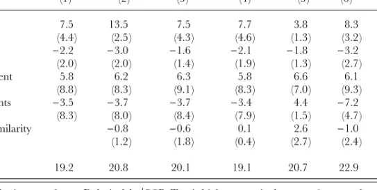
How likely is a debt crisis to infect the banking system? How exposed are banks to public debt? Data on public debt holdings by banks are hard to obtain. Table 2 shows data for 1992. We focus on national public debt as a share of bank assets (in the first panel), although the picture is essentially the same when we consider bank holdings of public debt as a percentage of GDP (in the second panel). The share of public debt in bank portfolios tends to be higher where the government is heavily
Table 2. Bank exposure to national public debt (NPD) and real estate loans (REL), 1992
Bank holdings % of bank assets % of GDP % of public debt Memo item: Public debt as % of GDP
NPD REL NPD REL NPD REL
Austria 23 48 52 Finland 39 France 1 14 2 19 5 39 Germany 4 9 31 34 Greece 9 12 105 Ireland 8 6 11 8 12 8 92 Italy 17 20 19 106 Netherlands 11 17 62 Norway 2 32 1 25 42 108 23 Spain 12 14 17 20 42 48 41 Sweden 2 35 3 71 8 160 67 Switzerland 29 72 16 UK 1 10 2 24 3 70 34
Notes: For Ireland real estate is personal house mortgage finance; for Sweden data concern all credit institutions. Final column refers to central government debt.
Source: National central banks; government statistical yearbooks.
11Central government debt is 12% of bank assets in Spain and 8% in Ireland, yet such debt is 105% of GDP in Ireland, but only 23% in Spain.
12These are averages for all banks (for more details, see Dalheim et al., 1992).
indebted, as in Italy and the Netherlands, although there are exceptions to the rule.11
How much public debt is too much? One comparison is with house price fluctuations in the late 1980s and early 1990s, exposure to which created serious problems for European financial institutions; in Nordic countries it forced governments to rescue the banks. Table 2 compares bank exposure to real estate loans with bank exposure to public debt. By this measure, exposure to public debt is not obviously a problem. At the time of the Nordic crisis in 1992, the BIS estimates that the share of bad loans in banks’ portfolios was 7.7% in Finland, 8.3% in Sweden and 9.3% in Norway (BIS, 1993). Suppose we conclude that the loss of 5% of bank assets was enough to cause severe distress and force the authorities to intervene.12 Were a government fully to default on its debt, exposure of 5% or more would be dangerous. Of course, governments rarely repudiate their debts; more typically they restructure, limiting capital losses for bondholders. Even if the capital loss associated with restructuring were 50% of the face value of the debt, only bank exposure in excess of 10% would be dangerous. By this measure, only Italy and Spain face significant risk of bank failure for debt-related reasons.
Debt default could still be a problem if the banks’ customers rather than the banks themselves hold the bulk of the debt. Default might incite households and
non-bank firms holding bonds to scramble for liquidity, and the ensuing withdrawal of deposits might create liquidity problems. It is instructive to consider the response of the Federal Reserve to the collapse of stock prices in 1929 and again in 1987. In both instances monetary policy was eased despite the fact that US financial institutions directly held only small amounts of stock. The Fed’s fear on both occasions was that financial distress would lead to defaults by brokers and other bank customers that would impair the capital position of the banks. In both cases, however, the liquidity injected into the financial system was smoothly withdrawn once the crisis passed; the consequences were deflationary, not inflationary.13 Similarly, banking crises in Sweden, Norway and Finland and serious problems for the banking system in France, Spain and Switzerland were all associated with deflation, not inflation, despite pervasive intervention by governments to rescue the banking system.
5. WOULD DEFAULT BY AN EMU MEMBER DEMORALIZE EMU BOND MARKETS?
A second channel through which debt problems in one jurisdiction can spill over to another is contagion in the bond market itself. If information is asymmetric, one debtor’s default may lead investors to revise downwards their expectations of maintenance of debt service by others. Debtors will find themselves having to accept higher yields to place new issues or to induce investors to roll over maturing ones. In so far as adverse consequences follow for the entire European bond market and not just the market in assets of the country in which the problem originates, pressure for the ECB to head off the problem will be intense.
This seems unlikely in Europe. Compared, say, to Latin America, information about governments’ willingness and ability to pay is relatively complete. It is unlikely that default or near default by one EMU country will per se lead investors to sharply higher expectations of default in another. This is logically distinct from the question of what might cause debt problems in an EMU country (election of a fiscally irresponsible politician, an asymmetric shock or an asymmetric response to a common shock); here we are concerned not with the causes of default, but with the scope for contagion.
From this point of view, a good analogy for post-EMU Europe may be the US market in state and municipal bonds. Not only is information relatively complete,14
13Subsequent research has found no role for fiscal profligacy in either crisis; indeed, scholarly accounts of the Great Depression blame excessively contractionary monetary policy. Neither suggests that a stability pact would have been helpful.
14
Especially in so far as tax advantages lead the vast majority of a state’s bonds to be held by its residents, who are in a good position to monitor the state’s economy and government.
but the USA is also a monetary union and individual states lack individual central banks to underpin their bond markets. The US market for state bonds has been analysed extensively: Goldstein and Woglom (1994) and Bayoumi et al. (1995) have studied yield spreads on state bonds issued between 1981 and the 1990s.
An objection to the use of these state and municipal data is that they pertain to lightly indebted governments. Both because 49 of the 50 state governments operate subject to statutory and constitutional fiscal constraints of varying severity and because their tax bases are relatively mobile, they have a limited capacity to incur and support high volumes of debt. Gross state debt to gross state product ratios are around 3%, far below the 70% debt ratio that characterizes the EU. Without substantial debts, US states have not experienced substantial debt problems; one would not expect to observe contagion. Yet US states rely on a smaller tax base than the European governments. Table 3 shows statistics on the ratio of public debts to the tax base (approximated by public spending). The difference between the two sets of governments remain sizeable, but less than the debt/income ratios.
While this objection has merit, US data are the only game in town. Nor is it true that statutory and constitutional restrictions prevented states and municipalities from running into trouble – recall New York City in the 1970s and Orange County in the 1990s. US states might have light debt loads, but having highly mobile tax bases, they also have limited capacity to raise taxes once a fiscal problem arises. Bayoumi et al. (1995) estimate that states get rationed out of the capital market when their debt/gross state product ratios approach 9%.
5.1. Event-study analysis
If contagion is present in a bond market like the USA, it may be a danger in post-EMU Europe. We therefore look for evidence that state-specific interest rate shocks have indeed been transmitted to neighbouring US states. Ideally, the original shock should be large, exogenous and state specific. We identified the ten largest changes in annual yield spreads (i.e., those at least two standard deviations above the mean change).15 All spreads are defined relative to the yield on New Jersey’s general Table. 3 Public debt as % of public spending
Average Minimum Maximum
51 US states (1990) 15 3 41
EU14 (1996) 158 102 250
Note: EU14 is without Luxembourg. Sources: Bayoumi et al. (1995) and OECD.
15Alabama, Michigan, Minnesota, Rhode Island, Washington and Wisconsin in 1982, New Hampshire in 1983, Texas in 1986, Louisiana in 1987 and Massachusetts in 1990.
obligation bonds, since this is how they are provided by the source. In most cases we were able to identify events leading to extraordinary increases in yields. Some of these were plausibly exogenous (the effect of the downturn in the auto industry on Michigan in 1982, the effect of falling oil prices on Louisiana in 1987). But neither the recession of the early 1980s nor the oil price decline of the late 1980s had effects limited to an individual state. For these, sympathetic increases in bond yields elsewhere could reflect that common shock rather than contagion per se.
One case where the shock was large, exogenous to the bond market and plausibly state specific was Washington State in 1982, where a major power district ran into serious trouble, servicing bonds issued for the construction of nuclear power plants (see Box 3). We concentrated on this case. We re-estimated the equations of Bayoumi et al. (1995), explaining the determinants of yield spreads to control for observable economic and demographic characteristics of states, and examined the residuals.16 Washington State had a large positive residual of 57 basis points in 1982. There was also a large positive residual for Oregon (20 basis points), consistent with contagion, even after controlling for changes in the debt burden,
16Bayoumi et al. (1995) relate the observed yield spread to the level of debt (as a percentage of gross state product, or GSP), the taxation of state bonds, the rate of unemployment and the strength of constitutional controls on state borrowing.
Box 3. Whoops! Washington State under nuclear stress
The 1982 shock to the Washington State bond market emanated from problems with servicing the obligations of the Washington Public Power Supply System (WPPSS). While these were not general obligation bonds, they represented one of the largest US bond defaults in history, and there was considerable uncertainty for a time about whether the state would assume responsibility for these obligations. WPPSS had been established in 1957 by a consortium of some two dozen small municipal utilities, whose initial goal was to build a hydroelectric plant and a steam generating plant, among other projects, to serve the member utilities. In 1970 WPPSS made a huge leap in scale and technology, beginning construction of five nuclear power plants. The small utilities involved had no experience of large-scale power projects, much less nuclear power. By the early 1980s they had incurred enormous cost overruns. In 1982 the bonds issued to finance the construction of Nuclear Units 4 and 5 lapsed into default. The event found immediate reflection in the yields on Washington State’s bonds. These increased by more than 70 basis points between 1981 and 1982, in the single largest increase in the ten-year sample.
unemployment, tax rates and so forth. But several other states also had positive residuals in 1982 at least as large as Oregon’s, including Delaware, Florida, Massachusetts, Michigan, Minnesota and Rhode Island; it is hard to see why any of them should have been especially strongly affected by difficulties in Washington State.
Other, unobservable, characteristics of states influencing yields could conceivably account for these patterns. To control for unobservables that are constant over time, we examined the change in the residuals from the yield spreads equation between 1981 and 1982. While the increase in the residual from the spreads equation is large and positive for Washington (51 basis points), it is now negative for Oregon. Positive increases of at least 25 basis points in the residual were also observed in Minnesota, Michegan and Rhode Island; decreases of at least 25 basis points in Pennsylvania as well as Oregon. As a final test, we examined states other than Washington that were also constructing nuclear power plants. Again the results were negative: there were neither unusually large residuals nor unusually large changes in the residuals in such states in 1982. Nothing in this analysis provides much evidence of interstate contagion.
5.2. Econometric analysis
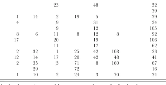
To analyse contagion in the US state and municipal bond market more systemati-cally, we re-estimated the Bayoumi et al. model, adding a measure of interest rate shocks in ‘economically contiguous states’.17 If the coefficient on the relevant measure of economic contiguity, when interacted with interest rates in neighbouring states, is positive, we have evidence of contagion. The critical step, obviously, is to measure economic proximity, the economic neighbours from which interest rate spillovers are most likely to spread. We consider a variety of specifications, appending them to Bayoumi et al.’s basic specification (column (1) of Table 4). In this basic specification, the spread increases with the ratio of debt to gross state product (heavier debt burdens increasing default risk), declines with the highest marginal tax rate in the state (a higher tax rate creating a captive market for bonds, income on which is tax exempt for local investors), rises with the state unemploy-ment rate (in so far as this implies less tax capacity) and falls with the stringency of self-imposed fiscal restrictions (which imply less debt accumulation in the future). All four regressors included in the basic specification are significant at conventional confidence levels.18
17Bayoumi et al. are concerned with non-linearities in the relationship between spreads and the level of debt; but while their non-linear specification allows them to capture the possibility of credit rationing, it also introduces instability into the model. We therefore focused on a linear version of their preferred specification. The basic results turn out to be quite similar to those of Bayoumi et al.
In the first of our augmented regressions (column (2)), we assume that interest rate spillovers are most likely to spread from states with similar debt burdens (as a share of gross state product): markets may interpret higher debt costs in one state as a signal of impending difficulties in states with similar debt levels. For each state in each year, we calculate the average yield in the four states with the most similar debt burdens, taking the two states just below and the two states ranked just above, using the debt/GDP ranking. We treat the average spread in these neighbouring states as endogenous to reflect common shocks as well as spillovers from a state to its neighbours. In column (2) the coefficient on ‘economic similarity’, having the wrong sign and being insignificantly different from zero, lends no support to the hypothesis of contagion.
In column (3) we consider a second definition of economic proximity based on federal aid per capita received. We apply the same procedure as for debt (selecting the two states immediately above and the two immediately below, using this ranking). Again we fail to detect significant contagion. The same result obtains using a third definition of proximity: the size of the state government measured as the ratio of state spending to GSP, in column (4).
Columns (5) – (7) focus on institutional constraints on fiscal policies, specifically the stringency of statutory and constitutional balanced-budget and debt-limitation provisions. The hypothesis, which seems plausible a priori, is that states are most subject to contagion from other states that use similar institutional procedures to Table 4. Bond market contagion in US states
Baseline Similarity: Similarity: Similarity: Similarity: fiscal restraints debt/GSP Federal aid govt size
N` 6 N` 7 N` 10 (1) (2) (3) (4) (5) (6) (7) Debt 7.5 13.5 7.5 7.7 3.8 8.3 5.4 (4.4) (2.5) (4.3) (4.6) (1.3) (3.2) (2.7) Tax −2.2 −3.0 −1.6 −2.1 −1.8 −3.2 −1.3 (2.0) (2.0) (1.4) (1.9) (1.3) (2.7) (1.0) Unemployment 5.8 6.2 6.3 5.8 6.6 6.1 5.7 (8.8) (8.3) (9.1) (8.3) (7.0) (9.3) (8.4) Fiscal restraints −3.5 −3.7 −3.7 −3.4 4.4 −7.2 −6.7 (8.3) (8.0) (8.4) (7.9) (1.5) (4.7) (5.8) Economic similarity −0.8 −0.6 0.1 2.6 −1.0 −1.0 (1.2) (1.8) (0.4) (2.7) (2.4) (2.0) SER 19.2 20.8 20.1 19.1 20.7 22.9 20.7
Notes: t-statistics in parentheses. Debt is debt/GSP. Tax is highest marginal tax rate in states that impose different tax rates on in-state and out-of-state bonds. Fiscal restraint indexed from 0 (none) to 10 (maximum). Unemployment and fiscal restraints treated as exogenous. Estimated by 2SLS using as instruments: average household size, population, change in population, proportion of young and old, trend GSP. All statistics computed with White heteroscedastic consistent procedure. 380 observations. Source: Bayoumi et al. (1995) pooled time series (1981 – 95) over 33 US states.
formulate their fiscal policies, since such states would be expected to respond similarly to similar disturbances. Bayoumi et al. (1995) utilize an index of the stringency of institutional restraints on fiscal policy constructed by the Advisory Commission on Intergovernmental Relations (discussed further in Eichengreen, 1990), which ranges from 1 to 10 in increasing order of severity. Unfortunately, states are not uniformly distributed over this interval. Of the 38 states in Bayoumi et
al.’s sample, seventeen have the maximum score of 10, while another seven have a
ranking of 8 or 9. Hence, using the same procedure as before to identify states would yield indeterminate or arbitrary results. We therefore consider states only with rankings N and below, assigning a value of zero for states ranked above, and then we allow N to take several values from 5 to 9.
The results are in columns (5) to (7). For N = 5, we detect some evidence of contagion via our economic similarity measure, but for larger values of N the effect is negative not positive: higher yield spreads in states with similar budgetary institutions lead to lower yields in states with similar fiscal arrangements, as if the markets, when they grow concerned by a state’s finances, shift their holdings so as to maintain a balanced portfolio of risks.
We also investigated whether there is contagion between ‘politically similar’ states.19 We define political proximity by the party affiliation of the governor, and construct a proximity dummy that takes a value of 1 when two governors are both Democrats or both Republicans (and zero otherwise). We then multiply the previous economic proximity variables by this dummy. Since rerunning the regressions in Table 4, replacing economic proximity by the above measure of economic and political proximity, made little difference to the broad pattern of results, we do not report these results separately. Indeed, in the few cases in which proximity variables that had previously been insignificant now became significant, their sign was negative, again suggesting portfolio diversification rather than contagion. The experience of US states provides no evidence to justify European-wide fiscal restraints to protect against contagious bond market crises.
6. WOULD EXCESSIVE DEFICITS PUSH UP EMU INTEREST RATES?
In EMU, within which capital is mobile, borrowing by one country is likely to have only a small effect on EMU interest rates: European countries borrow on global capital markets, relative to which they are individually small. Even if a country’s actions raise its own interest rates – for example, through a larger risk premium – there is little reason (contagion apart) why this should imply substantial cross-border spillovers.
19
Note that we condition political proximity on economic proximity. Unconditional political proximity is unlikely to be a sharp classification if about half the governors are Democrats and the other half are Republicans.
6.1.Evidence from the financial markets
The ideal way to verify this hypothesis would be to build a structural model of savings and investment for each European country, taking account of the influence of both domestic and foreign variables, and distinguishing of-Europe and rest-of-world magnitudes. This is ambitious to say the least. Here we take the simpler tack of estimating the reduced-form relationship between interest rates, asking whether interest rates in a particular European country are affected mainly by own values, rest-of-Europe values or rest-of-world values.
The straightforward way of implementing this analysis is with Granger causality tests. Two prior decisions that must be made are what countries and what interest rates to analyse. But no one would be surprised if our results showed that interest rates in Luxembourg were affected by interest rates in the rest of the world and in the rest of Europe, but that interest rates in Luxembourg affected those in neither the rest of Europe nor the rest of the world. We therefore bias the results against our own hypothesis by considering the impact of rest-of-world and rest-of-Europe interest rates on Germany, and the impact of German interest rates on those of the rest of the world and the rest of Europe.
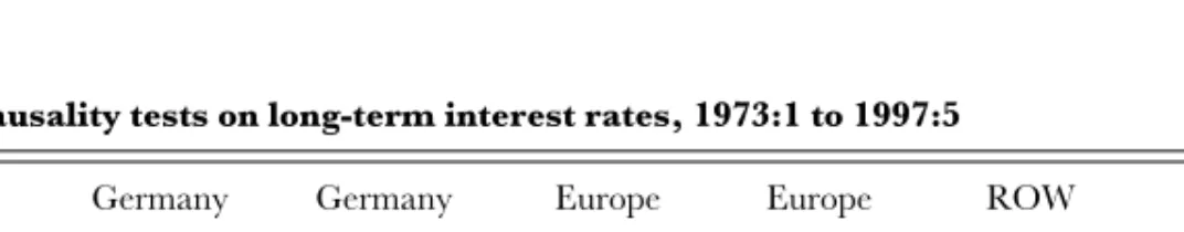
Similarly, if the analysis concerned itself with co-movements in short-term interest rates, no one would be surprised if we found evidence of Granger causality running in both directions, since these timing relationships could reflect not just market spillovers but also the induced policy reaction of central banks, which use short-term interest rates as policy instruments (Wyplosz, 1990). We therefore focus on the behaviour of long-term interest rates, whose co-movements are less likely to be dominated by induced central bank reactions and are more likely to convey information about market spillovers.20
Table 5. Causality tests on long-term interest rates, 1973:1 to 1997:5
Germany Germany Europe Europe ROW ROW
causes causes causes causes causes causes
Europe? ROW? Germany? ROW? Germany? Europe?
F-statistic 1.9 1.4 2.2 2.0 3.2 2.4
Probability (%) 3.9 14.4 1.3 2.8 0.0 0.7
Notes: Tests with 12 lags (choice implied by Akaike and Schwartz criteria). Europe is GDP-weighted average of Austria, Belgium, Denmark, France, Ireland, Italy, Netherlands, Spain, UK. Rest of the world (ROW) is weighted average of Canada, Japan and USA.
Source: IMF, International Financial Statistics.
20
Since long rates are an average of the current and expected future short rates, this does not eliminate the possibility that the correlations we pick up are in part central bank reactions, but it should minimize that possibility.
We used monthly data, current and lagged up to twelve months, on treasury bond rates for Germany, the rest of Europe (a weighted average of nine European countries listed in the note to Table 5, weighted by 1985 GDP) and the world (proxied by interest rates for the USA, Canada and Japan, again weighted by 1985 GDP). At the 1% level, we can reject all spillovers except that rest-of-world interest rates affect European interest rates and that rest-of-world interest rates affect German interest rates: once we control for world interest rates, innovations in German rates do not affect interest rates in the rest of Europe, and innovations in rest-of-Europe rates do not affect German rates. The only other relationship that approaches significance at the 1% level is the impact of rest-of-Europe rates on Germany. In each case, then, it is the larger entity whose interest rates affect those of the smaller economy.
These tests confirm that European countries borrow on a global capital market, with only small interest rate spillovers between EMU members. They hardly justify a stability pact to internalize cross-border interest rate spillovers of national fiscal policy.
7. WOULD THE PACT INCREASE THE VOLATILITY OF EMU OUTPUT?
We address this question in two steps. We use retrospective evidence to ask how frequently the Stability Pact would have been binding, and we use counterfactual simulations to estimate how European output would be affected if binding Stability Pact ceilings were imposed. Inevitably this exercise is subject to the Lucas critique: evidence from the past may not be a reliable guide to the future. We go some way towards answering this objection by adjusting historical debt ratios and interest rates to the levels likely to prevail at the outset of EMU, basing our simulations on these adjusted values.
7.1 Retrospective evidence
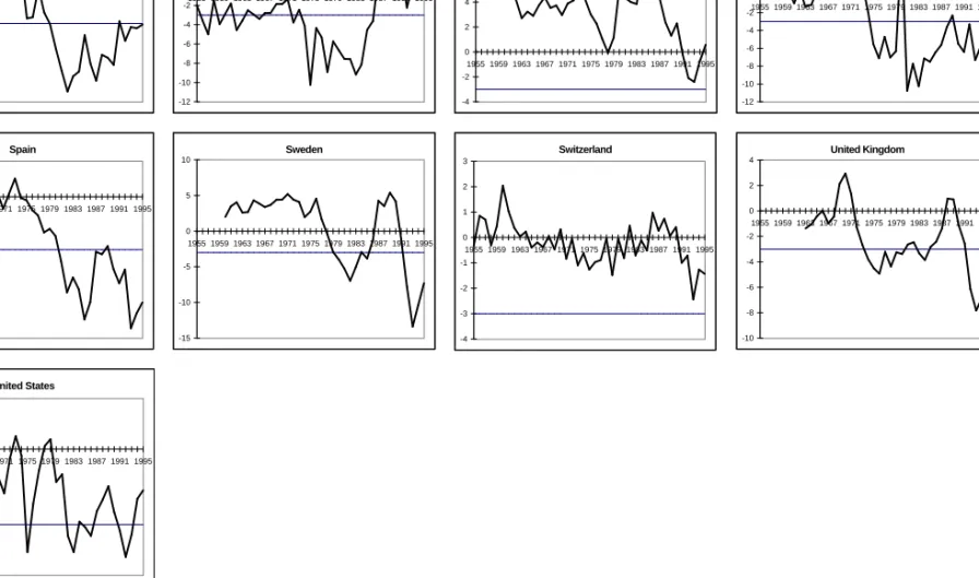
Figure 1, which shows budget balances for OECD countries since 1955, documents that the 3% barrier has been breached quite frequently.21 (A similar analysis, reaching the same conclusions, is provided by Buti et al., 1997). Table 6 shows that this has been the case 34% of the time for the OECD as a whole, and 40% of the time in Europe.
Of the 241 cases when the deficit was more than 3% of GDP, in only 7 was the concurrent decline in GDP more than 2%, and in only 28 was it more than 0.75%.
21
The Maastricht Treaty includes a particular definition of deficits that may differ slightly from the data from
BARRY EICHENGREEN AND CHARLES WYPLOSZ Ireland -14 -12 -10 -8 -6 -4 -2 0 1955 1959 1963 1967 1971 1975 1979 1983 1987 1991 1995 Italy -14 -12 -10 -8 -6 -4 -2 0 1955 1959 1963 1967 1971 1975 1979 1983 1987 1991 1995 Japan -6 -4 -2 0 2 4 1955 1959 1963 1967 1971 1975 1979 1983 1987 1991 1995 Greece -16 -14 -12 -10 -8 -6 -4 -2 0 1955 1959 1963 1967 1971 1975 1979 1983 1987 1991 1995 France -7 -6 -5 -4 -3 -2 -1 0 1 2 1955 1959 1963 1967 1971 1975 1979 1983 1987 1991 1995 Germany -6 -5 -4 -3 -2 -1 0 1 2 3 4 1955 1959 1963 1967 1971 1975 1979 1983 1987 1991 1995 Denmark -10 -8 -6 -4 -2 0 2 4 6 1955 1959 1963 1967 1971 1975 1979 1983 1987 1991 1995 Finland -10 -8 -6 -4 -2 0 2 4 6 8 10 1955 1959 1963 1967 1971 1975 1979 1983 1987 1991 1995 -14 -12 -10 -8 -6 -4 -2 0 1955 1959 1963 1967 1971 1975 1979 1983 1987 1991 1995 Belgium Canada -8 -6 -4 -2 0 2 4 1955 1959 1963 1967 1971 1975 1979 1983 1987 1991 1995 -5 -4 -3 -2 -1 0 1 2 1955 1959 1963 1967 1971 1975 1979 1983 1987 1991 1995 Australia -7 -6 -5 -4 -3 -2 -1 0 1 2 3 1955 1959 1963 1967 1971 1975 1979 1983 1987 1991 1995 Austria
89 -7 -6 -5 -4 -3 -2 -1 0 1 1955 1959 1963 1967 1971 1975 1979 1983 1987 1991 1995 -4 -2 0 2 4 6 8 1955 1959 1963 1967 1971 1975 1979 1983 1987 1991 1995 -12 -10 -8 -6 -4 -2 0 2 4 6 1955 1959 1963 1967 1971 1975 1979 1983 1987 1991 1995 Spain -8 -7 -6 -5 -4 -3 -2 -1 0 1 2 1955 1959 1963 1967 1971 1975 1979 1983 1987 1991 1995 Sweden -15 -10 -5 0 5 10 1955 1959 1963 1967 1971 1975 1979 1983 1987 1991 1995 -12 -10 -8 -6 -4 -2 0 2 4 1955 1959 1963 1967 1971 1975 1979 1983 1987 1991 1995 Switzerland -4 -3 -2 -1 0 1 2 3 1955 1959 1963 1967 1971 1975 1979 1983 1987 1991 1995 United Kingdom -10 -8 -6 -4 -2 0 2 4 1955 1959 1963 1967 1971 1975 1979 1983 1987 1991 1995 United States -5 -4 -3 -2 -1 0 1 2 1955 1959 1963 1967 1971 1975 1979 1983 1987 1991 1995
Figure 1. Budget balances (% of GDP)
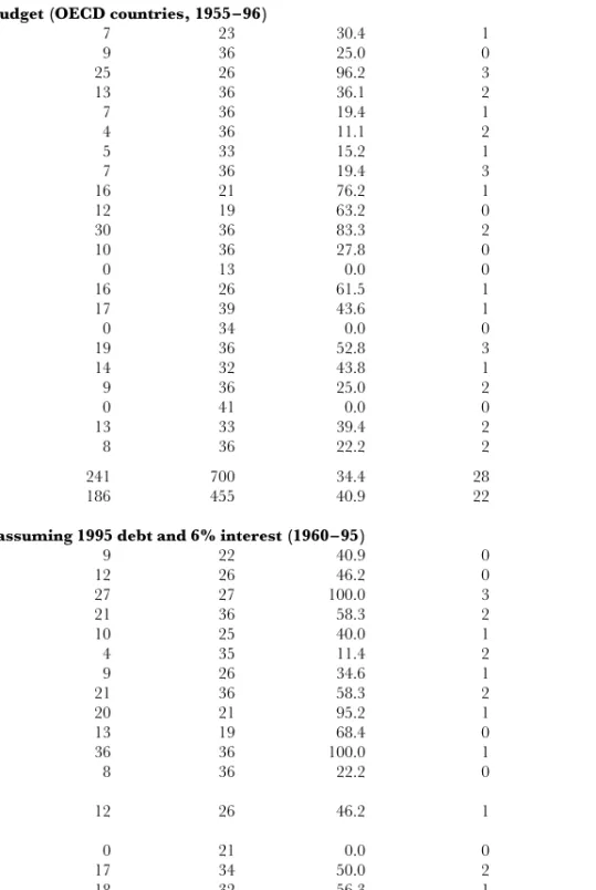
Table 6. Number of times the deficit exceeded 3% of GDP
Number of Total Percentage Recession years years observations above 3%
Above 0.75% Above 2%
(a) Actual budget (OECD countries, 1955 – 96)
Australia 7 23 30.4 1 0 Austria 9 36 25.0 0 0 Belgium 25 26 96.2 3 0 Canada 13 36 36.1 2 1 Denmark 7 36 19.4 1 0 Finland 4 36 11.1 2 1 France 5 33 15.2 1 0 Germany 7 36 19.4 3 0 Greece 16 21 76.2 1 0 Ireland 12 19 63.2 0 0 Italy 30 36 83.3 2 1 Japan 10 36 27.8 0 0 Luxembourg 0 13 0.0 0 0 Netherlands 16 26 61.5 1 0 New Zealand 17 39 43.6 1 1 Norway 0 34 0.0 0 0 Portugal 19 36 52.8 3 1 Spain 14 32 43.8 1 0 Sweden 9 36 25.0 2 1 Switzerland 0 41 0.0 0 0 UK 13 33 39.4 2 0 USA 8 36 22.2 2 1 All countries 241 700 34.4 28 7 EU countries 186 455 40.9 22 4
(b) Budget assuming 1995 debt and 6% interest (1960 – 95)
Australia 9 22 40.9 0 0 Austria 12 26 46.2 0 0 Belgium 27 27 100.0 3 0 Canada 21 36 58.3 2 1 Denmark 10 25 40.0 1 0 Finland 4 35 11.4 2 1 France 9 26 34.6 1 0 Germany 21 36 58.3 2 0 Greece 20 21 95.2 1 0 Ireland 13 19 68.4 0 0 Italy 36 36 100.0 1 1 Japan 8 36 22.2 0 0 Luxembourg Netherlands 12 26 46.2 1 0 New Zealand Norway 0 21 0.0 0 0 Portugal 17 34 50.0 2 1 Spain 18 32 56.3 1 0 Sweden 10 26 38.5 2 1 Switzerland UK 12 26 46.2 1 0 USA 17 36 47.2 3 1 All countries 276 546 50.5 23 6 EU countries 221 395 55.9 18 4
Note: Recession years are counted only when the budget deficit exceeds 3% of GDP. Source: OECD Economic Outlook.
Had OECD countries been operating with the Stability Pact, 85% of the deficits that exceeded 3% of GDP would have been judged excessive.22 Put differently, we can calculate the probability of observing a deficit in excess of 3% of GDP conditional
on there being no recession. When a recession is defined as a decline in annual real
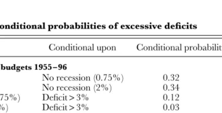
GDP of at least 0.75%, the conditional probability is 32%, rising to 34% when recession is defined as a 2% decline (Table 7). If the past is a guide, we can expect violations every third year. The constraint imposed by the Stability Pact appears even more stringent when we realize that the conditional probability of observing a recession when the budget deficit exceeds 3% is only 12% if the recession corresponds to the 0.75% definition, and 3% for the 2% definition.
One can argue that this record is evidence of the need for constraints to prevent misbehaviour. Indeed, the common interpretation of the Stability Pact is that it will lead member countries to aim at budgets that are on average in balance, or slightly positive. With a budget in surplus at the peak of cycle, it will be possible to use fiscal policy as a counter-cyclical tool. What is wrong with that? A first response – the second one is presented below in section 8 – is that the ‘misbehaviour’ documented in Table 7 did not have the dramatic inflationary consequences of concern to proponents of the Stability Pact. Average annual inflation for the same sample of countries was a relatively moderate 6% over the period. This 6% may be more inflation than some Europeans would like, but it is hardly the inflationary disaster feared by some EMU-sceptics. Pooling the data for all countries, the partial correlation between inflation and the budget deficit is negative (though not significant), contradicting the assumption that deficits are associated with inflation.
Table 7. Conditional probabilities of excessive deficits
Event Conditional upon Conditional probability
Using actual budgets 1955 – 96
Deficitp 3% No recession (0.75%) 0.32
Deficitp 3% No recession (2%) 0.34
Recession (0.75%) Deficitp 3% 0.12
Recession (2%) Deficitp 3% 0.03
Assuming 1995 debt level and 6% interest rate
Deficitp 3% No recession (0.75%) 0.49
Deficitp 3% No recession (2%) 0.50
Recession (0.75%) Deficitp 3% 0.08
Recession (2%) Deficitp 3% 0.02
Source: Authors’ calculations based on Table 6.
22Our approach does not exactly match the criteria of the Stability Pact which apply to the previous four quarters, since we have to look at calendar years (fiscal data are widely reported only on an annual basis).
7.2. Counterfactual evidence
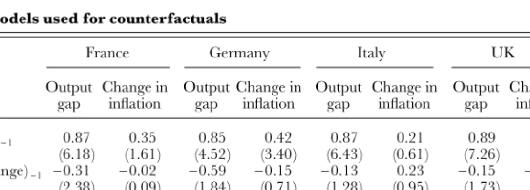
Can we gauge the consequences of having subjected the European economies to the Stability Pact for the last 30 years? One approach involves estimating, for the four largest countries (France, Germany, Italy and the UK), a simple structural model. The simplest structural macroeconomic model of all, of course, is the textbook model of an upward-sloping aggregate supply curve and a downward-sloping aggregate demand curve in the output – price space. Fiscal policy, among other variables, shifts the demand curve. We measure the fiscal stance by the fiscal impulse, the year-to-year change in the cyclically adjusted budget deficit. This allows us to minimize the risk that an observed correlation between the deficit and output captures the impact of output on the budget, rather than the impact of the budget on output, with which we are concerned. Allowing for some inertia in both relationships, we get the reduced form for output and inflation in Table 8.23 In order to impose the restriction that fiscal policy has no steady-state effect, we use the output gap and the change in the inflation rate along with the fiscal impulse measure. The output gap and the cyclically adjusted budget are taken from the OECD Economic Outlook.
23Note the parallel between these reduced forms and standard VARs, since output and inflation both depend on their own lagged values. The policy inferences that we make from these equations are subject to standard critiques (see Cochrane, 1994). We finesse some but not all of these objections by using the cyclically adjusted budget as opposed to the actual budget deficit. In addition, we worry about the possibility that the fiscal impulse variable is systematically correlated with monetary policy, thus biasing the estimate of its coefficient. A check is to look for subsample stability. Performing Chow tests with a break in 1985, to account for a change in the policy mix when monetary discipline was introduced in the EMS, we can reject at the 5% confidence level (and in most cases at the 1% confidence level) the hypothesis that the estimates change from one subperiod to the other.
Table 8. Models used for counterfactuals
Coefficient France Germany Italy UK
(t-statistic)
Output Change in Output Change in Output Change in Output Change in gap inflation gap inflation gap inflation gap inflation
(Output gap)− 1 0.87 0.35 0.85 0.42 0.87 0.21 0.89 0.58 (6.18) (1.61) (4.52) (3.40) (6.43) (0.61) (7.26) (2.25) (Inflation change)− 1 −0.31 −0.02 −0.59 −0.15 −0.13 0.23 −0.15 −0.16 (2.38) (0.09) (1.84) (0.71) (1.28) (0.95) (1.73) (0.88) Fiscal impulse −0.68 0.09 −0.58 −0.33 −0.43 1.28 0.69 0.51 (3.03) (0.26) (2.11) (1.79) (1.73) (2.52) (2.03) (1.07) Adjusted R2 0.71 0.43 0.51 0.39 0.74 0.12 0.69 0.26 SER 0.01 0.02 0.02 0.01 0.01 0.03 0.02 0.04 Source: OECD.
Notes: Fiscal impulse is change in cyclically adjusted budget surplus; for France and the UK this variable is
The coefficient on the fiscal impulse shows the impact of the budget on the out-put gap. This coefficient is similar across our sample, ranging from −0.43 in Italy to −0.68 in France; thus, for each of the four countries, an increase in the cyclically adjusted surplus by 1% of GDP lowers the output gap by roughly 0.5% of GDP.
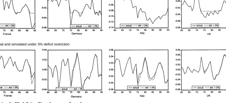
These equations are used for counterfactual simulations in which the budget deficit is capped at 3%, as if the Stability Pact had been strictly binding. The top row of Figure 2 shows the actual budget balance in our four countries (the solid line) and the counterfactual deficits capped at 3% of GDP (the broken line). French deficits would have been different only in the early 1980s, under the first Mitterrand government, and in the 1990s. German deficits would have been smaller in the wake of the two oil shocks and to a lesser extent following unification. Italy, the high-deficit country in our sample, would have had very much smaller high-deficits since the early 1970s, while the UK would have had somewhat smaller deficits over the same period, with the exception of the second half of the 1980s.
The bottom row of Figure 2 shows the effect in our estimated model of restricting the budget deficit to a maximum of 3%. It displays the actual output gap (the solid line) and the counterfactual gap from a simulation where the deficits are capped at 3%, as shown in the top row (the broken line). A fair characterization is that Stability Pact ceilings on deficits would have mattered for output, but not dramatically so. (Box 4 discusses the extreme cases.) Table 9 compares the average actual and simulated output gaps. In each country but Germany the output gap is lower when the deficit is capped; while the slowdown is not large, even a fraction of a percentage point on the annual growth rate can become a big effect when it lasts over decades. This is shown by cumulating the gaps over the 22-year period 1974 – 95: the output losses range from about 5% in France and the UK to 9% in Italy, significantly larger than optimistic estimates of favourable output effects to be expected from EMU. For example, the EU Commission’s report One Market, One
Money (1990) set its central estimate of the gross gains at 9.8% of GDP.
Further-more, in each case but Germany, the variability of output as measured by the standard deviation is higher under the counterfactual. The tempting political-economy inference is that Germany is particularly insistent on a 3% cap on deficits because historically it alone among the four large EU member states would not have suffered too seriously from the imposition!
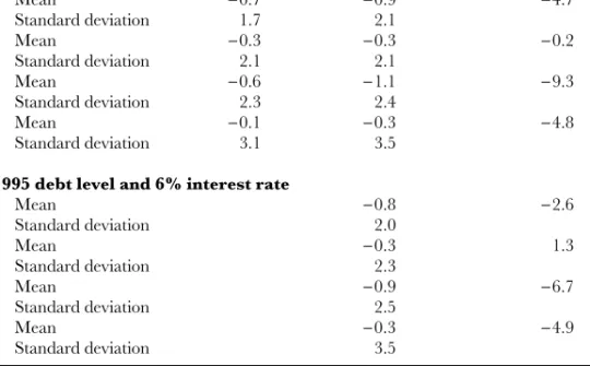
It can be objected that these simulations do not provide a reliable guide to the future because historical time series do not capture fiscal conditions as they will exist at the beginning of EMU. Simulations and conditional probabilities based on historical data are an imperfect guide to the future because debts are higher now than historically and because (nominal) interest rates will be lower at the start of EMU than over the last twenty years. If we adjust debts and interest rates to levels likely to prevail in 1999 (we use 1995 debt/GDP ratios and nominal interest rates of 6% (2% inflation + 4% real interest), this has the predictable effect of raising the probability of a deficit in excess of 3%. The bottom part of Table 7 showed that,
BARRY EICHENGREEN AND CHARLES WYPLOSZ
Budget balance: actual and restricted (deficit not to exceed 3% of GDP)
Output gap: actual and simulated under 3% deficit restriction
Sources: OECD and authors’ calculations.