Ishikawa, or cause-and-effect diagrams, help to visualize the parameters that influence a chromatographic analysis. Therefore, they facilitate the set up of the uncertainty budget of the analysis, which can then be expressed in mathematical form. If the uncertainty is calculated as the Gaussian sum of all uncertainty parameters, it is necessary to quantitate them all, a task that is usually not practical. The other possible approach is to use the intermediate precision as a base for the uncertainty calculation. In this case, it is at least necessary to consider the uncertainty of the purity of the reference material in addition to the precision data. The Ishikawa diagram is then very simple, and so is the uncertainty calculation. This advantage is given by the loss of information about the parameters that influence the measurement uncertainty.
Introduction
The complete mathematical description of a chromatographic separation is nearly impossible because the process is influenced by an enormous number of parameters, many of them of complex in nature, such as the interplay of mobile and stationary phases (1). As a consequence, the comparison of the sample signal with the signal of a well-known reference is necessary for quantitative analysis. This can be the peak area or height.
The influence parameters and their interplay can be visualized by Ishikawa or cause-and-effect diagrams (2). In a tree-like struc-ture, the parameters with their “causes“ that lead to an “effect” of any kind are drawn in a logical manner. The norm ISO 9004-4 gives the following description (3): “a cause-and-effect diagram is used to analyze cause-and-effect relationships; to communicate cause-and-effect relationships; and to facilitate problem solving from symptom to cause to solution”.
Drawing an Ishikawa diagram increases the understanding of how an analytical method works. In addition, it is helpful in set-ting up an uncertainty budget (4). By today’s standards, the result of a quantitative analysis should be accompanied by its measure-ment uncertainty value (5); how this can be calculated is explained in the EURACHEM/CITAC Guide (6) and the superordi-nated Guide to the Expression of Uncertainty in Measurement (7). Thus far, many analysts still have difficulties with the
deter-mination of measurement uncertainties, and this paper shows how this task can be handled.
The contribution presents different diagrams and the respec-tive uncertainty equations for the area of a single peak, compar-ison of reference and sample peaks (single-point calibration), comparison when the intermediate precision is known, and an analysis performed with multiple-point calibration. For most val-idated analyses, the long-term repeatability or intermediate pre-cision is known. This leads to a great simplicity for the calculation of the combined measurement uncertainty because, in many cases, it is only the uncertainty of the purity of the reference material that needs to be considered additionally, as will be shown.
Experimental
Parameters of a liquid chromatographic analysis that influence the uncertainty
Most chromatographic analyses include a number of working steps, such as weighing, pipetting, dilution, and extraction opera-tions, later followed by the separation on a column. These proce-dures are needed for both the sample and reference (although in many cases, the latter is treated in a simpler way, including only the weighing of a standard, dilution, and injection). Moreover, what needs to be known is the purity (or content) of the reference material and the recovery of the sample preparation. In order to understand the Ishikawa diagrams, the uncertainties of the working steps and of the other influence quantities are discussed first.
Mass
The uncertainty of a mass (m) determination (i.e., a weighing operation) is influenced by the repeatability (Rep), the nonlin-earity of the characteristic curve of the balance (NL), the sensi-tivity (or slope) tolerance (S), the temperature coefficient of the sensitivity (TC), and the uncertainty of the buoyancy by weighing in air (BU) (8). These parameters are independent of each other and their linkage is additive, therefore the total uncertainty [u(m)] is calculated in accordance with the Gaussian law of error propagation:
Abstract
Measurement Uncertainty of Liquid Chromatographic
Analyses Visualized by Ishikawa Diagrams
Veronika R. Meyer
Eq. 1 The detailed uncertainty budget of a mass determination is more complicated than suggested by equation 1 because some parameters are a function of the net weight, whereas others depend on the gross weight. The relative uncertainty [u(m)rel] is
usually in the range of 10–500 ppm of the net weight. Buoyancy is a systematic, though small, effect (bias) that should be consid-ered for the highest accuracy. If performed correctly, mass deter-minations are the most precise operations in the laboratory, as long as the weighing good is not critical (such as humid, hygro-scopic, or electrically charged) and the uncertainties [u(m)] are negligibly small in the uncertainty budget of a chromatographic analysis.
Purity
A reference compound has a certain purity (Pur) and an uncer-tainty of the purity. There are no mandatory rules of how to cal-culate the uncertainty of a stated purity such as 99.8% ± 0.1%, ≥ 97%, etc. (9). The simplest possibility is to treat the range as a tri-angular or recttri-angular distribution (10). For a statement of the type ± x%, it is reasonable to choose the triangular distribution, and the standard uncertainty becomes:
Eq. 2A If the purity is indicated in the form ≥ y%, it is better to define the range (100–y)% as the limits of a rectangular distribution; then the standard uncertainty is:
Eq. 2B A reference purity value of less than 100% (Pur < 1) is a sys-tematic effect that must be considered for the calculation of the analytical result.
Recovery
If a sample preparation by extraction is necessary, the recovery (Rec) is less than 100%, in many cases. The uncertainty of the recovery is equal to the standard deviation (s) calculated from the n-fold investigation of this step (11):
u(Rec) = s(Rec) Eq. 3
There is no general consensus if an analytical result shall be corrected by the recovery factor (12). Some guidelines or official methods require it, whereas others outlaw such a correction. Dilution
The dilution (Dil) of a sample or reference is usually made with pipets and measuring flasks. Their volumes have a multiplicative linkage; it is possible to define a dilution factor Dil as the product of all pipet volumes divided by the product of all flask volumes. If n pipets and m measuring flasks are involved, Dil and the total uncertainty [u(Dil)] are calculated as follows:
Eq. 4A
Eq. 4B Each volume uncertainty [u(V)] is composed of the indepen-dent parameters calibration (Cal), repeatability (Rep), and uncer-tainty of the temperature (T) (strictly speaking, the influence of the temperature on the thermal expansions of liquid and volu-metric device):
Eq. 5 With volumetric instruments, calibration and repeatability are combined to the maximum permissible error (MPE); this value is printed on glass instruments after the “±” sign, or can be found in the norm for piston-operated pipets (13,14). Equation 5 is reduced to:
Eq. 6 The relative uncertainty [u(V)rel] of a single volumetric
opera-tion (pipetting or dissolving to a given volume) is in the range of 10/
00for diluted aqueous solutions. The relative uncertainty of a
dilution, performed with three consecutive operations, then adds up to 1.70/
00with Equation 4B. (Three operations are necessary
when a mass is weighed, diluted to x mL in a measuring flask, then y mL are taken with a pipet and diluted to z mL in another flask. Dil has the unit mL–1in this case). For volumes in the
low-microliter range and for solvents other than water, the uncer-tainty can reach 1% or more.
Injection volume
The uncertainty parameters of the injected volume (V) are the repeatability, the calibration of the autosampler or syringe, and the uncertainty of the temperature. The combined uncertainty is calculated with equation 5.
High-performance liquid chromatography
The uncertainty of the separation process has contributions from the separation (mobile phase, stationary phase, column dimensions, and more), from the detection (in the case of UV detection there are, for example, the time constant and the wave-length accuracy), and from the integration [integration parame-ters, signal-to-noise ratio (s/n), peak shape, and more]. The individual uncertainties of these influence parameters vary between minor and remarkable; a gradient separation with ion-pair reagent is more prone to interferences than a normal-phase separation with a one-component eluent. Separation, detection, and integration are also characterized by their individual repeata-bilities. Although a more detailed uncertanty calculation is pos-sible, in principle (15), it is not practicable and the uncertainty of a high-performance liquid chromatographic (HPLC) separation (or another chromatographic separation) is characterized by its overall repeatability (short-term) or reproducibility (long-term, perhaps with the use of different columns or different batches of mobile phase, etc.), expressed as relative standard deviation:
u(HPLC)rel= s(HPLC)rel Eq. 7
This experimental standard deviation includes not only the sep-u(m) =
√
u2(Rep) + u2(NL) + u2(S) + u2(TC) + u2(BU)u(Pur) =
√
6 x u(Pur) =√
3 2 100 – y Dil = VPip,i/ VMF,j i=1 j=1 n mII
II
u(Dil) u(VPip,i)
VPip,i Dil i=1 n 2
Σ
= +√
( )
j=1 u(VVMF,jMF,j) m 2Σ
( )
u(V) = u
√
2(cal) + u2(Rep) + u2(T)aration process but also the uncertainty of the injection volume. Area of a liquid chromatographic peak
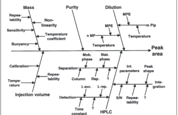
Although a complete mathematical description of the chro-matographic process is not available, it is possible to set up a prag-matic equation for the area of a peak. We assume that a certain mass of a compound (e.g., the reference) is weighed in, dissolved in a solvent, diluted, injected, and separated by HPLC. The result is a peak with an area that is integrated. The area (A) can be described as follows:
A = m · Pur · Dil · V · HPLC Eq. 8
where m = mass of a chemical compound, Pur = purity of this compound, Dil = dilution factor, V = injection volume, and HPLC = empirical response factor that describes the relationship between injected mass and peak area. Equation 8 leads to the drawing of the Ishikawa diagram shown in Figure 1. Each factor of the equation is represented by a side branch of the main arrow, and the ramification can be continued to any wanted degree. Figure 1 is drawn with the goal of the uncertainty determination. Therefore, the factors that influence the uncertainty are shown. In the HPLC branch, a number of question marks are noted because it would be difficult to define and present an exhaustive number of influence factors.
The combined relative standard uncertainty of the peak area is not a direct representation of equation 8 because the repeatability of the injection volume is included in the standard deviation of repeated HPLC separations and u(V) disappears. Equation 8 is multiplicative in character, therefore the relative uncertainties need to be squared for the calculation of the combined standard uncertainty:
Eq. 9 Note: for a gas chromatographic (GC) peak, the HPLC branch in the Ishikawa diagram needs to be replaced by a GC branch with its parameters. The only difference of the diagram as shown in Figure 1 is that the detection has nothing to do with a wavelength but, for example, with the characteristics of a flame-ionization detector. One of the characteristics of the mobile phase in GC is its temperature, whereas in HPLC it is the composition (not drawn for better clarity).
Comparison of two chromatographic peaks
The direct comparison of two peak areas (or heights) is made when a quantitative analysis is based on single-point calibration. The peak obtained by the injection of a sample solution is com-pared with the one generated by the reference solution. The pre-requisite is that the empirical response factor (called HPLC in equation 8) is identical for the two peaks. With regard to the sample peak, we assume that a certain amount of sample is weighed in, followed by dilution or extraction steps (or both). The extraction or other sample preparation procedures have a certain recovery. Finally, the sample is injected and separated by HPLC.
A simple comparison of peak areas is based on the concentra-tions of the analyte in the injected soluconcentra-tions:
Eq. 10 where c = concentration, V = injection volume, and A = peak area. What is needed to be known is, however, the analyte concentra-tion in the sample as it was weighed in. The complete mathemat-ical description is as follows:
Eq. 11 It is a good practice to inject identical volumes of sample and reference solution because then the calibration of the autosam-pler or syringe is no longer important. Equation 11 can be replaced by:
Eq. 12 What is still relevant for the uncertainty calculation is the repeatability of the injection including the possible temperature fluctuation between injections. However, the accuracy of the detection wavelength is irrelevant and only its repeatability from one injection to another is a point that influences the uncertainty. As long as the HPLC instrument is running smoothly and the sample and reference solutions are investigated within a short time interval, most influence parameters such as the eluent com-position, stability of the stationary phase, retention factor, and so on, can be looked at as constant in a first approximation. They are identical for sample and reference, even peak shape and s/n are similar when both peaks have similar size (which should be the case with single-point calibration) and when the chromato-graphic resolution is adequate. This leads to a simplification of the lower half of Figure 1. The former injection volume and HPLC branches can be combined to a peak area branch that has only repeatability terms (Figure 2).
The combined relative standard uncertainty of the analyte con-centration in the sample is:
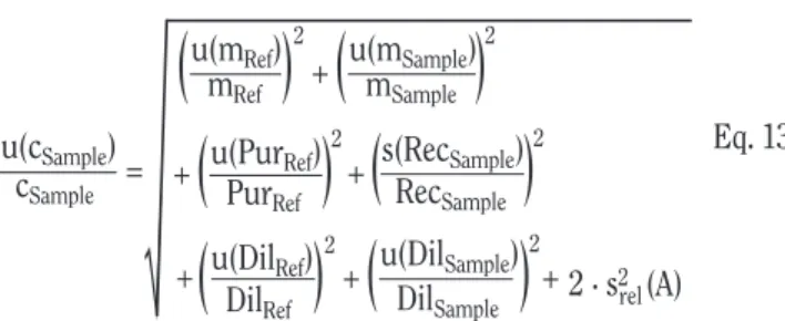
Eq. 13
with m = mass, Pur = purity, Rec = recovery, Dil = dilution factor, and A = peak area. The unit of cSampleis g/g or another mass/mass
expression.
In many cases, the dilution schemes for sample and reference are not identical, therefore the individual dilution factors and their uncertainties appear in equation 13. When the areas of both peaks are of similar size, their uncertainties (expressed as standard devi-ations) are all but identical and can be combined to 2s2(A).
It is obvious that it is impossible in a quality control laboratory to differentiate between the uncertainties of the injection (16), separation, detection, and integration (and in a research labora-tory this task would be difficult). Moreover, in many cases there is no time and interest to determine the repeatability of peak areas.
u(A) u(m) A m 2
√
( )
= + u(Pur) Pur 2(
)
+ u(Dil) s2 (HPLC) Dil rel 2(
)
+ CSampleSolution=CRefSolution· VRef· ASample
VSample· ARef
CSample=
mRef· PurRef· DilRef · ASample
mSample· RecSample· DilSample· VSample· ARef
CSample=
mRef· PurRef· DilRef · VRef· ASample
mSample· RecSample· DilSample· ARef
u(cSample) u(mRef) u(DilRef) DilRef mRef 2 cSample = + +
√
(
(
)
2)
u(mSample) mSample 2(
)
+ s(RecSample) RecSample 2(
)
+ + (A) rel u(PurRef) PurRef 2 · s2 2(
)
+ u(DilSample) DilSample 2(
)
What is known is the repeatability or reproducibility of the whole analytical procedure.
Single-point calibration with known intermediate precision Equation 12 is valid for many types of chromatographic anal-yses with single-point calibration, either “single shots” in the research laboratory or well-established routine investigations. When an analytical procedure is planned to be used in the rou-tine, a thorough validation is necessary. In addition, its long-term reproducibility is known after some time by observing the peak area of the analyte, obtained by the injection of either a pure ref-erence compound or of a matrix refref-erence material after the work-up procedure. The best overview about the variability of this peak area is obtained by a control chart (17).
This long-term reproducibility is identical with the interme-diate precision of the analysis. It covers different batches of mobile and stationary phases, different temperatures in the labo-ratory, and different volumetric instruments with their individual calibration that were used for the dilutions. If different balances are used, their individual sensitivity tolerances and nonlinearities are also included in the reproducibility. If a matrix reference material is used, the repeatability of the sample preparation is included in the reproducibility, as well.
Figure 3 shows the influence factors that need to be considered for the uncertainty calculation aside from the reproducibility. The parameters with dashed arrows are present or absent, as explained previously. The uncertainty equation becomes:
Eq. 14A
when a reference compound with purity (PurRef) is used, and:
Eq. 14B
when a matrix reference material with analyte content (ContRef)
is used. Rep is now reproducibility (i.e., the intermediate preci-sion), not repeatability. For chromatographic analyses, the repro-ducibility is in the 1% range or even much larger (e.g., in the case of trace analysis or in clinical chemistry). The relative uncertain-ties originating from mass determinations are often in the 10–100-ppm range (as already explained), therefore they can be neglected in this case. This leads to the uncertainty equations for the two strategies:
Eq. 15A
Eq. 15B
Example with reference compound
The purity of the reference compound is stated by the manu-facturer as Pur ≥ 98%. With Equation 2B, an uncertainty u(Pur) = 0.58% is obtained. The recovery should be determined with approximately ten investigations; it was found to be 0.84 (84%) with a standard deviation of 0.03. The long-term relative repeata-bility of the reference peak is 0.018 (1.8%). Equation 15A gives:
Figure 2. Ishikawa diagram for an HPLC analysis with single-point
calibra-tion. What needs to be determined is the concentration of the analyte in the sample. For the abbreviations, see Figure 1. The new letters are Rec = recovery and A = peak area.
Figure 3. Ishikawa diagram for the uncertainty of an analysis with single-point
calibration with an unknown reproducibility. Depending on the set-up of the reproducibility determination and on the given situation in the laboratory, the influence factors with dashed arrows are or are not included in the overall reproducibility. (Note: as explained later in the text, this diagram is also valid for analyses with multiple-point calibration and linear regression).
u(cSample) u(mRef) mRef 2 cSample = +
√
(
)
u(mSample) mSample 2(
)
+ s(RecSample) RecSample 2(
)
+ + rel u(PurRef) PurRef Rep2 2(
)
u(cSample) cSample =√
s(RecSample) RecSample 2(
)
+ + rel u(PurRef)PurRef Rep
2 2
(
)
u(cSample) cSample =√
+ rel u(ContRef)ContRef Rep 2 2
(
)
u(cSample) u(mRef) mRef 2 cSample = +√
(
)
u(mSample) mSample 2(
)
+ u(ContRef) ContRef 2(
)
+ rel Rep2Figure 1. Ishikawa diagram for an isolated chromatographic peak.
Abbreviations: n MF = number of measuring flasks, m Pip = number of pipets, λ = wavelength, rep. = repeatability, and acc. = accuracy.
Eq. 16
Example with matrix reference material
The content of the reference material is 50 µg/g, guaranteed with extreme values of ± 5 µg/g. u(Cont) is calculated with Equation 2A and gives 2.0 µg/g. The long-term repeatability of the analyte peak obtained from the worked-up matrix reference mate-rial is 0.075 (7.5%). Equation 15B gives:
Eq. 17
Multiple-point calibration with known intermediate precision
A multiple-point calibration is usually performed with linear regression. The concentration of the analyte in the sample is cal-culated by:
Eq. 18 with a = y-axis intercept (usually in mV) and b = slope (e.g., in mV × mL/µgwhen the x-axis is in concentration units). The influence parameters mRef, PurRef, and DilRefare “hidden” in the x-axis and
therefore also in the slope. The determination of the uncertainty of a linear regression is not straightforward (18–20). If, however, the intermediate precision of the analytical method is known (including repeated determinations of the calibration function), equations 14 and 15 are also valid in this case, as well as Figure 3.
Conclusion
The measurement uncertainty of a quantitative analysis based on the comparison with a reference material is not described by its reproducibility alone. It is necessary to consider also the uncertainty of the purity or content of the reference material and, depending on the set-up, perhaps also the uncertainty of the sample preparation step (i.e., the uncertainty of the recovery). This is also true for nonchromatographic analyses such as spec-troscopic assays [i.e., in general for relative (nonprimary) analyt-ical methods]. An equation of the type 15 is very simple and the combined standard uncertainty of the analysis can easily be cal-culated from validation data plus some additional information. The drawback of this approach, often referred to as the “top-down” method, lies in the fact that the numerous influence fac-tors that lead to the overall reproducibility are not known numerically. As a consequence, the knowledge about how the combined standard uncertainty of an assay could be lowered is rudimentary.
Acknowledgments
I am indebted to my colleague Dr. Roman Hedinger for fruitful
discussions and new insights into the topic of measurement uncertainty related to HPLC analyses.
References
1. V.J. Barwick. Sources of uncertainty in gas chromatography and high-performance liquid chromatography. J. Chromatogr. A 849: 13–33 (1999).
2. K. Ishikawa. “Cause-and-Effect Diagrams”. In Introduction to Quality
Control. Kluwer, Dordrecht, the Netherlands, 1991, chapter 4.7.4,
pp. 229–33.
3. British Standard. ISO 9004-4. Total Quality Management. Part 2.
Guidelines for Quality Improvement. CEN, Brussels, Belgium, 1993,
ISBN 0-580-22865-7.
4. S.L.R. Ellison and V.J. Barwick. Estimating measurement uncertainty: reconciliation using a cause and effect approach. Accred. Qual.
Assur. 3: 101–105 (1998).
5. European Standard, EN ISO/IEC 17025. General Requirements for
the Competence of Testing and Calibration Laboratories.
CEN/CEN-ELEC, Brussels, Belgium, 1999.
6. S.L.R. Ellison, M. Rösslein, and A. Williams, Eds. EURACHEM/CITAC
Guide, Quantifying Uncertainty in Analytical Measurement, 2nd ed.
2000, ISBN 0-948926-15-5. Free download from: http://www.mea-surementuncertainty.org/mu/guide.
7. International Organization for Standardization. Guide to the
Expression of Uncertainty in Measurement. ISO, Geneva,
Switzerland, 1995, ISBN 92-67-10188-9.
8. A. Reichmuth. “Weighing accuracy with laboratory balances”. In
Proc. 4th Biennial Conference of the Metrology Society of Australia.
2001, pp. 38–44.
9. G. van Look and V.R. Meyer. The purity of laboratory chemicals with regard to measurement uncertainty. Analyst 127: 825–29 (2002). 10. International Organization for Standardization. Guide to the
Expression of Uncertainty in Measurement, subclause 4.3. ISO,
Geneva, Switzerland, 1995, ISBN 92-67-10188-9, pp. 11–14. 11. V.R. Meyer. Comments on species-specific isotope dilution-based
calibration for trace element speciation and its combined uncertainty evaluation: determination of tributyltin in sediment by HPLC-ICPMS.
Anal. Chem. 75: 1552 (2003).
12. M. Parkanyi, Ed. The Use of Recovery Factors in Trace Analysis. Royal Society of Chemistry, Cambridge, U.K., 1996.
13. International Standard, ISO 384. Laboratory glassware, Principles of
design and construction of volumetric glassware. ISO, Geneva,
Switzerland, 1978.
14. International Standard. DIN EN ISO 8655. Piston-operated
volu-metric apparatus. ISO, Geneva, Switzerland, 2002.
15. V.J. Barwick, S.L.R. Ellison, C.L. Lucking, and M.J. Burn. Experimental studies of uncertainties associated with chromato-graphic techniques. J. Chromatogr. A 918: 267–76 (2001). 16. K.G. Kehl and V.R. Meyer. Argentometric titration for the
determina-tion of liquid chromatographic injecdetermina-tion reproducibility. Anal.
Chem. 73: 131–33 (2001).
17. E. Mullins. Introduction to control charts in the analytical laboratory.
Analyst 119: 369–75 (1994).
18. EURACHEM/CITAC Guide, Quantifying Uncertainty in Analytical
Measurement, Appendix E.3.
19. J. Vian and A. Jardy. Taking into account both preparation and injec-tion in high-performance liquid chromatography linearity studies. J.
Chromatogr. Sci. 38: 189–94 (2000).
20. E. Achermann and O. Chinellato. Estimating Measurement
Uncertainty, Technical Report 346, Department of Computer
Science, ETH Zurich, Switzerland, 2000. Free dowload from: http://www.inf.ethz.ch/publications.
Manuscript accepted July 10, 2003.
u(cSample) cSample =
√
+ 2.0 µg/g 50 µg/g 0.0752= 0.085 = 8.5% 2(
)
cSample= (ASample– a)mSample· RecSample· DilSample· b
u(cSample) cSample =