HAL Id: hal-03070554
https://hal.archives-ouvertes.fr/hal-03070554
Submitted on 15 Dec 2020
HAL is a multi-disciplinary open access archive for the deposit and dissemination of sci-entific research documents, whether they are pub-lished or not. The documents may come from teaching and research institutions in France or abroad, or from public or private research centers.
L’archive ouverte pluridisciplinaire HAL, est destinée au dépôt et à la diffusion de documents scientifiques de niveau recherche, publiés ou non, émanant des établissements d’enseignement et de recherche français ou étrangers, des laboratoires publics ou privés.
to disease treatment
Ninon Burgos, Simona Bottani, Johann Faouzi, Elina Thibeau-Sutre, Olivier
Colliot
To cite this version:
Ninon Burgos, Simona Bottani, Johann Faouzi, Elina Thibeau-Sutre, Olivier Colliot. Deep learning for brain disorders: from data processing to disease treatment. Briefings in Bioinformatics, Oxford University Press (OUP), 2021, 22 (2), pp.1560-1576. �10.1093/bib/bbaa310�. �hal-03070554�
Briefings in Bioinformatics
Special Issue on Deep Learning
Deep learning in brain disorders: from data processing
to disease treatment
Ninon Burgos*,1,2,3,4,5; Simona Bottani*,1,2,3,4,5; Johann Faouzi*,1,2,3,4,5;
Elina Thibeau-Sutre*,1,2,3,4,5; Olivier Colliot†,1,2,3,4,5
1 Paris Brain Institute, F-75013, Paris, France 2 Inserm, U 1127, F-75013, Paris, France 3 CNRS, UMR 7225, F-75013, Paris, France 4 Sorbonne Université, F-75013, Paris, France
5 Inria Paris, Aramis project-team, F-75013, Paris, France *Equal contribution
†Corresponding author:
Olivier Colliot Paris Brain Institute ARAMIS team
Pitié-Salpêtrière Hospital
47-83, boulevard de l’Hôpital, 75651 Paris Cedex 13, France E-mail: [email protected]
Abstract
In order to reach precision medicine and improve patients’ quality of life, machine learning is increasingly used in medicine. Brain disorders are often complex and heterogeneous, and several modalities such as demographic, clinical, imaging, genetics and environmental data have been studied to improve their understanding. Deep learning, a subpart of machine learning, provides complex algorithms that can learn from such various data. It has become state-of-the-art in numerous fields including computer vision and natural language processing, and is also growingly applied in medicine. In this article, we review the use of deep learning for brain disorders. More specifically, we identify the main applications, the concerned disorders and the types of architectures and data used. Finally, we provide guidelines to bridge the gap between research studies and clinical routine.
Keywords:
deep learning, neurology, medical imaging, genomicsSummary key points
● Deep learning has been applied to various tasks related to brain disorders, such as image reconstruction, synthesis and segmentation, or disease diagnosis and outcome prediction. ● Convolutional neural networks have been successfully applied to imaging and genetic data in
numerous brain disorders, while recurrent neural networks showed encouraging results with longitudinal clinical data and sensor data.
● Despite the promising results obtained with deep learning, several important limitations need addressing before an application in clinical routine becomes possible.
● Future research should especially focus on the generalizability and interpretability of deep learning models.
1. Introduction
Precision medicine, as a customization of healthcare, aims at providing specific care to each individual. Examples of precision medicine include providing the right diagnosis as early as possible, giving the most appropriate treatment, and predicting the evolution of the disease for a specific patient. As disorders and patients are both highly heterogeneous, precision medicine requires gaining knowledge about the disorders that may be too complex to be feasible for a human being.
Machine learning allows computers to perform tasks (for instance, predicting patient survival) without having to explicitly provide rules. Instead, machine learning algorithms learn to perform a task by adjusting their parameters using training data. The trained model can then be applied on new unseen data to evaluate its performance. Standard machine learning, such as generalized linear models, support vector machines and tree-based algorithms, relies on pre-extracted features that are assumed to well-characterize the samples. These features can be subjective, domain-specific and highly engineered. They are extracted using predefined procedures designed using expert knowledge (one often refers to them as “handcrafted” features even though the feature extraction procedures are most often automatic). Deep learning (DL), a subpart of machine learning, consists of algorithms that can learn features themselves. In such approach, the algorithm is usually an artificial neural network where the different neurons are organized into layers. Specifically, deep learning refers to the use of networks with a large number of layers. For both theoretical and practical approaches on deep learning, we invite the readers to have a look at [1–3].
In order to achieve precision medicine and gain more knowledge about disorders, machine learning is increasingly used in medicine [4–8]. As it can deal with diverse data, such as imaging and genetic data, DL is growingly applied in fields such as cellular and medical imaging, genomics or drug discovery [9–15].
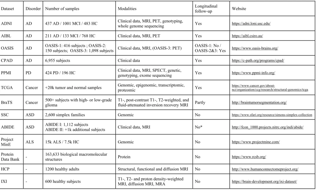
This review will enable readers to grasp the full potential of DL for brain disorders as it presents the main uses of DL all along the medical data analysis chain: from data acquisition to disease treatment. We first focus on data processing, covering image reconstruction, signal enhancement and cross-modality image synthesis (section 2) and on the biomarkers that can be extracted from spatio-temporal neuroimaging data, such as the volume of normal structures or of lesions (section 3). We then describe how DL can be used to detect diseases (section 4), predict their evolution (section 5), improve their understanding (section 6) and help develop treatments (section 7). For these applications, we emphasize the types of architectures and data used, as well as the concerned disorders. Finally, we highlight trending applications (section 8) and provide guidelines to bridge the gap between research studies and clinical routine (section 9). Table 1 lists the acronyms and abbreviations used throughout the manuscript and Table 2 proposes a selection of the most frequently used and richer publicly available datasets. Summaries of the studies reviewed in sections 2 to 8 are available in supplementary materials (Tables S1 – S7).
2. Data reconstruction and preprocessing
2.1. Image reconstruction
Deep learning has been used for medical image reconstruction to enable shorter acquisitions (magnetic resonance imaging (MRI), positron emission tomography (PET)) and/or reduce radiation
dose (PET). The idea of using artificial neural networks to reconstruct images is not recent [16–18] but is currently a very active field of research, see [19] for a review.
Raw MRI data are samples of the Fourier transform of the object being imaged. The image can thus be reconstructed by performing an inverse Fourier transform operation on the raw data. One of the main shortcomings of MRI is the long scanning time. MRI acquisition acceleration can be achieved by only partially filling the k-space (i.e. the frequency space). The information loss can then be compensated by using parallel imaging, and various techniques have been developed to enable the reconstruction from under-sampled k-spaces and circumvent aliasing artifacts. As for the classic approaches, DL reconstruction approaches can operate at the k-space or at the image level, but they can also operate both at the space and image levels, or directly learn the transformation from k-space to image k-space [20]. The majority of the DL methods operate at the image-level [21–35] with the networks learning a mapping from aliased images, reconstructed from under-sampled k-spaces using the inverse Fourier transform, to de-aliased images. The de-aliased image can be the final product [23,25,27,24,31,32,35], be used as input of classic approaches [21] or be combined with the initial under-sampled k-space before a refinement step [26,28,34]. The network architecture can also be designed to mimic a classic iterative reconstruction where steps of reconstruction and DL-based regularization alternate [22,29,30,33]. Several approaches aim to improve k-space interpolation [36,37]. In [36], the network is trained on an autocalibrating signal specific to each scan, while in [37] it is trained offline using pre-acquired images. The method described in [38] operates at both the k-space and image levels by alternating between steps of k-space completion and image restoration. Finally, the approach proposed by Zhu et al. [39] learns the complete mapping from k-space data to the reconstructed image. Note that DL has also been used for MRI fingerprinting, to learn the mapping between the set of images acquired with different scan parameters (flip angle, repetition time, echo time) and parametric maps [40–42].
Deep learning can also be used to recover high quality PET images acquired with a reduced dose. As previously, the majority of the techniques operate at the image level, the network learning a mapping between low dose and high dose images [43–51]. While several methods rely only on the PET images to learn this mapping [43–46], others use MR images acquired simultaneously with the PET data on PET/MR scanners as input [47–49]. In the previous works, neural networks were applied post reconstruction, but they can also be integrated within the iterative reconstruction [50,51]. Alternatively, Sanaat et al. [44] proposed to predict a high dose sinogram (the Radon transform of the image) from a low dose sinogram, which appears to lead to higher quality images compared to the prediction in the image domain. More generally, several works aim at directly learning the mapping between sinograms and images [39,52,53], as neural networks are expected to enable the automatic optimization of the image reconstruction algorithms and be computationally more efficient than the classic techniques.
2.2. Signal enhancement
Many of the reconstruction techniques operating in the image domain could be considered as image denoising approaches as image translation is performed post-reconstruction. Denoising can be applied more generally on various modalities, for brain applications mainly MRI [54–56] and PET [57,58]. Both images [55,57] and spatio-temporal signals [54,56,58] can be denoised.
Another image enhancement technique is super-resolution. Most approaches rely on pairs of high- and low-resolution images of a single modality to learn the low- to high-resolution mapping [59–64]. Others do not use external training data. The self super-resolution method presented in [65]
assumes that in-plane MRI slices have a high resolution and can therefore be used as high-resolution training data. By degrading the in-plane slices into low resolution images, a neural network can be trained and then used to restore the images in the through-plane. Another self super-resolution strategy consists in combining multiple images of the same subject, one low-resolution and the other high-resolution, to improve the resolution of the former [66–68].
2.3. Cross-modality image synthesis
Image translation has also been used in a cross-modality context, such as to generate computed tomography (CT) from MR images [69–84] or to generate MR images of a certain sequence from MR images of another sequence [74,85–90] or a set of other sequences [83, 91–97]. A large number of methods have been applied to improve attenuation correction on PET/MR scanners [73,76,78,81,98,99] or to enable radiotherapy treatment planning from MRI only [71,77,80,84]. Other studies aim to improve subsequent image processing steps such as segmentation or registration [90], improve classification in case of missing data [86,91,100,101], improve detection and segmentation of tumors [90,93] or white matter lesions [95,102], correct distortions in diffusion MRI [88] or enable MR-less PET quantification [103].
As can be seen in Table S1, the most common networks used for image reconstruction, signal enhancement and cross-modality image synthesis are variations of convolutional neural networks (CNN), the U-Net [104] and its variations, and conditional generative adversarial networks (GAN) (see Figure 1 for an illustration of several network architectures).
3. Extraction of biomarkers
Deep learning can be used to extract different types of biomarkers, such as the volume of normal structures or of lesions, or age predicted from neuroimaging data.
3.1. Segmentation of anatomical structures
Deep learning is widely used for the segmentation of normal structures from brain MR images. A general overview of the existing datasets, DL architectures and main results collected until 2017 is given in [105]. Two main segmentation strategies exist. In the sliding-window CNN framework, a network is trained to predict the class label of each pixel by providing a patch around that pixel as input. This approach was used in [106–108], where patches of different sizes were used as inputs to ensure spatial consistency, and in [109] where the CNN is combined with a Hough-voting strategy to perform anatomy localization. Other articles implement fully convolutional networks, with unimodal [110] or multimodal [111] data. Many adapt the U-Net architecture introduced by Ronneberger et al. [104], such as [112,113]. More recently, adversarial learning strategies have been used to force the automatic segmentations to resemble manual segmentations [114].
3.2. Segmentation of lesions
Beyond normal anatomical structures, segmentation of lesions, such as tumors, white matter hyperintensities and ischemic or hemorrhagic lesions, can provide key information for disease management. In particular, it allows tracking growth or reduction of lesions, which is essential to assess disease progression and treatment efficacy. As for the segmentation of anatomical structures,
U-Net like architectures are often employed. However, strategies aiming to particularly focus on lesions have been implemented. In the dual pathway CNN strategy, two image inputs first go through different convolutional blocks and are then merged in the fully connected layers. In the cascade CNN strategy, the output of a first CNN, trained to be more sensitive to potential voxels with lesions, is given as input to another CNN where the number of misclassified voxels is reduced.
Research on automatic segmentation and detection of brain tumors has been propelled by the availability of the Brain Tumor Segmentation (BraTS) challenge datasets [115,116], which include multimodal MR images for subjects with glioblastoma and lower grade glioma. For this application, the dual pathway strategy is widely used [117–122]. DeepMedic is one of the most common architectures [117]: it is a multiscale dual pathway network composed of two 3D CNN to take into account both local and global contextual information. It has also been adapted to segment traumatic brain injury lesions from multimodal MRI data [123]. Other works aiming to delineate brain tumors proposed cascade CNN architectures [124,125], an adaptation of the U-Net architecture [126], an encoder-decoder architecture with a variational autoencoder branch reconstructing the input images jointly with segmentation to regularize the shared encoder [127] or a sliding-window CNN framework [128,129]. Finally, segmentation of hyperspectral pictures (obtained with a visible and near-infrared pushbroom camera) was also used to help surgeons during tumor resection [130]. In this study, several DL methods (multilayer perceptron, CNN, U-Net) were assembled in one pipeline.
White matter lesion detection is often performed in the context of multiple sclerosis. Both the cascaded 3D CNN [131] and U-Net like [132] approaches have been explored. Guerrero et al. [133] proposed a U-Net like architecture for the segmentation and differentiation of white matter hyperintensities and stroke lesions from T1-weighted (T1w) and fluid-attenuated inversion recovery (FLAIR) MR images. Cerebral microbleeds, small hemorrhages near blood vessels, have been detected using a cascaded framework [134] and a 2D CNN [135].
3.3. Brain age
The so-called “brain age” approach can be used as a non-specific biomarker of different brain disorders. A model is optimized to predict the real (chronological) age of healthy controls (HC) from neuroimaging data. Then, abnormalities can be detected in patients if their predicted brain age differs from their chronological age. This has been observed for many brain disorders such as Alzheimer’s disease [136], epilepsy [137], multiple sclerosis [138], schizophrenia [139] or traumatic brain injury [140].
Many studies on that topic have been conducted by the same first author, James H. Cole. He proposed a DL system to predict age in healthy subjects [141], using a 3D CNN trained on gray matter, white matter or non-segmented T1w MRI. They compared their results to a standard machine learning method (Gaussian process regression) and observed that DL obtained comparable results for preprocessed data (gray matter and white matter) but significantly outperformed it for raw data. Their best mean absolute error was obtained with the CNN applied to gray matter. Jonsson et al. [142] proposed a similar framework with a 3D residual CNN and performed significantly better.
3.4. Identification of biomarkers in electroencephalography signals
Deep learning is also used to identify biomarkers in electroencephalography (EEG) signals. In [143,144], 2D CNN were applied to raw scalp EEG signals to perform a classification task. In [143] the goal was to detect P300 signals while spelling words, whereas in [144] the goal was to differentiate
EEG signals containing or not an epileptic seizure. In either case the input of the CNN is a matrix with rows corresponding to electrodes and columns to time points. In [143] weights of the convolutions were directly interpreted, while Hossain et al. [144] extracted correlation maps to find which channels are relevant. Finally, Schirrmeister et al. [145] proposed different methods to train CNN for EEG decoding and visualization that could be used for biomarker discovery.
4. Disease detection and diagnosis
Most of the studies on disease detection have dealt with Alzheimer’s and Parkinson’s diseases [146,147]. This is partly due to the public availability of large datasets such as from the Alzheimer’s Disease Neuroimaging Initiative (ADNI) and the Parkinson’s Progression Markers Initiative (PPMI) cohorts (more details in Table 2). The aim of disease detection and diagnosis can be to differentiate healthy controls from subjects with a disease or to distinguish between different diseases (disease recognition), but also, once a disease has been singled out, to quantify its severity or to differentiate between subtypes.
4.1. Disease recognition
Many studies focusing on Alzheimer’s disease aim to differentiate healthy controls from subjects with dementia, a relatively easy task useful when developing classification methods but clinically irrelevant [148]. The most commonly used approach is an end-to-end CNN for classification [146– 148]. Wen et al. [148] provided a review on the use of CNN for AD classification showing that results obtained with CNN are comparable to those obtained with traditional machine learning techniques. Nevertheless, other approaches exist. Silva et al. [149] used a CNN for feature extraction only and not classification. A variational autoencoder was used by Choi et al. [150] to detect anomalies in PET images, thereby providing a score of abnormality used to identify AD patients. The main imaging modalities used for AD classification are T1w MRI and 18F-fluorodeoxyglucose PET [147], but
others, for example amyloid PET, have been used [151]. Other types of data, such as speech data [152], also bring meaningful information.
Several studies have dealt with the classification of PD patients versus controls. This can be achieved using single-photon emission computed tomography [153], neuromelanin sensitive MRI [154], diffusion MRI [155] or handwriting images [156,157].
Differentiating healthy controls from subjects with a psychiatric disease is also a research question widely addressed. Depression was studied using EEG as input [158,159]. To overcome the lack of patient data, transfer learning was used in the work of Banerjee et al. [160], where they classified patients with post-traumatic stress disorder using a deep belief network model. Classification of schizophrenia versus HC is performed in several studies with a sparse multilayer perceptron [161], a deep discriminant autoencoder network [162], or a CNN combined with a pre-trained convolutional autoencoder [163], and classification of bipolar disorders versus HC is studied in [164] with a 3D CNN. The public availability of the Autism Brain Imaging Data Exchange dataset (Table 2) has propelled research on autism spectrum disorder. For example, functional MRI data were used in [165,166] to distinguish patients with an autism spectrum disorder from controls using a CNN. Other works used genomic data with a neural network [167] or eye tracking data with a long short-term memory (LSTM) [168]. A multimodal approach for the integration of functional and structural MRI was proposed by Zou et al. [169] for the classification of attention deficit hyperactivity disorder
versus healthy children using a 3D CNN. Finally, Zhang et al. [170] identified patients with conduct disorder using T1w MRI and a 3D variation of AlexNet.
The control versus disease task is not limited to neurodegenerative and psychiatric disorders. Classification of epileptic subjects versus HC has been addressed by Aoe et al. [171] who built a CNN called M-Net from magnetoencephalography signals. Fu et al. [172] performed natural language processing by using a CNN to detect individuals with silent brain infarction using radiological reports, as early detection can be useful for stroke prevention. Using different features extracted from functional MRI data, Yang et al. [173] proposed to distinguish between migraine patients and healthy controls (but also between two subtypes of migraine) using an Inception CNN. Finally, MR angiography was used to detect cerebral aneurysms [174,175] using a custom CNN [174] or a ResNet-18 [175].
Few studies have explored differential diagnosis with DL. Wada et al. [176] classified AD versus Lewy body dementia using a 2D CNN while Huang et al. [177] classified bipolar disorder versus unipolar depression using a CNN followed by an LSTM, both with attention mechanisms.
4.2. Identification of known disease subtypes
Neurological disorders can be complex, and several works aim to identify known disease subtypes or quantify their severity. This is particularly the case in oncology. In the brain cancer domain, most of the studies [178–180] focused on low-grade gliomas. Low-grade gliomas are less aggressive tumors with better prognosis compared to high-grade gliomas. In low-grade gliomas, the genetics of the tumor can provide prognostic information, but this analysis requires biopsy, which is an invasive procedure. To rely only on non-invasive examinations, these studies proposed DL methods to distinguish between different genetic classes based on structural MRI. Ge et al. [179] performed two classification tasks: low-grade versus high-grade gliomas (tumor grading) and low-grade gliomas with or without 1p19q codeletion, a biomarker predictive of chances of survival (tumor subtyping). They used a 2D CNN on T1w, T2w and FLAIR MRI slices. Akkus et al. [178] also performed the same tumor subtyping task using 2D CNN on T2w and post-contrast T1w MRI, and Li et al. [180] predicted the mutation status of isocitrate dehydrogenase 1 in low-grade gliomas using a 2D CNN associated with a support vector machine applied to post-contrast T1w and FLAIR MRI. Additionally, Hollon et al. [181] classified images of biopsies (stimulated Raman histology) between 13 common subtypes covering 90% of the diversity of brain tumors with a 2D CNN. They compared their workflow with pathologists interpreting conventional histologic images and achieved a similar diagnostic accuracy for a large gain in diagnostic time (less than 2.5 minutes versus 30 minutes). They also successfully identified rare phenotypes as they did not belong to any of their predefined classes, though they could not distinguish between them.
The distinction of disease subtypes has also been explored for other neurological disorders. Choi et al. [182] aimed to differentiate PD patients with dementia from those without dementia following a transfer learning strategy using a CNN initially trained to distinguish controls versus AD patients. In [183] the objective was to identify subtypes of PD progression using an LSTM with clinical and imaging data. Kiryu et al. [184] aimed to differentiate Parkinsonian syndromes. Different clinical profiles of patients with multiple sclerosis were identified in [185] using graphs extracted from diffusion MRI and graph CNN. Non-contrast head CT scanners were used by [186] for the detection of intracranial hemorrhage and its five subtypes. They used a CNN to identify the presence or absence of intracranial hemorrhage and a recurrent neural network for the classification of intracranial hemorrhage subtypes. In the context of epilepsy, Acharya et al. [187] used a CNN to
distinguish three classes of EEG signal: normal, preictal and seizure. San-Segundo et al. [188] studied two different tasks using a CNN applied to EEG: classification of epileptic versus non-epileptic brain areas and detection of epileptic seizures.
5. Disease prediction
This section focuses on the prediction of the future evolution of brain disorders. Three different protocols were implemented to perform such prediction: (i) binary classifications between participants who will develop or not the disease in a fixed time horizon, (ii) regression tasks estimating the time before disease development, and finally (iii) the generation of future imaging modalities.
5.1. Fixed-time classification
Studies in this section aim at predicting the progression of patients in a pre-defined time frame. The length of this time frame depends on the disease studied: a few minutes for epilepsy [189] to several years for multiple sclerosis [190] or Alzheimer’s disease [191–195].
For epileptic patients who are drug-resistant, the short-term prediction of a seizure could improve their quality of life and independence. In [189], scalp and intracranial EEG 30s-windows processed by a short-time Fourier transform were used to distinguish preictal (before seizure onset) from interictal (between seizures) phases with a 2D CNN. With a seizure prediction horizon of 5 minutes and an occurrence prediction of 30 minutes, the system is significantly better than a random predictor for both modalities.
In multiple sclerosis, the disease course can be highly variable and predicting the evolution of the patients in early stages is difficult. Yoo et al. [190] studied patients who presented early symptoms of multiple sclerosis and aimed to classify those whose condition would worsen within two years and those who would stay stable. To that purpose, they used lesion masks extracted from T2- and proton density-weighted MRI which were fed to a 3D CNN pre-trained in an unsupervised way.
In Alzheimer’s disease, a binary classification between stable mild cognitive impairment (sMCI) and progressive MCI (pMCI) allows the identification, as early as possible, of the patients who could benefit from a treatment. As most of these studies also tackled AD versus HC, their architectures were already described in section 4. Therefore, in this section we will only focus on transfer learning between these two tasks. Four possibilities were explored: i) transferring weights from AD versus HC and then fine-tuning on pMCI versus sMCI [191,192]; ii) transferring from a classification with the first class mixing AD and pMCI labels and the second class HC and sMCI labels, and then fine-tuning on pMCI versus sMCI [193]; iii) directly testing the network on pMCI and sMCI patients without fine-tuning after learning the AD versus HC classification [195]; and iv) directly learning sMCI versus pMCI classification [194]. It is important to note that the definition of the labels may vary between studies. Most of them chose a prediction horizon (18, 36 or 60 months) and labeled as pMCI patients who converted within this prediction horizon and as sMCI patients who have a follow-up of at least the prediction horizon and did not convert at any time. However, some studies chose to remove patients with insufficient follow-up, thereby complicating the classification task. The absence of a common definition of the labels makes the comparison between studies difficult.
5.2. Time-to-disease regression
Several studies have estimated survival time after diagnosis of brain cancer. Two studies [196,197] fused histological slices and genetic information from brain tumors. Patches of histological slices were processed by convolutional layers and genetic information was added at the level of the fully-connected layers [197] or processed in its own branch [196]. Mobadersany et al. [197] only included 1p19q codeletion and isocitrate dehydrogenase mutation status, which were the target classes of studies in section 4. Hao et al. [196] included more genetic data but allowed a restricted number of connections between the gene (first) layer and the pathway (second) layer, these restrictions being based on prior biological knowledge.
5.3. Longitudinal image prediction
Instead of predicting a diagnosis status relying on clinical assessments which may vary depending on the examiner and conditions of examination, one can predict future values of imaging modalities. In [198], a conditional GAN including two discriminators was used to predict the evolution of white matter hyperintensities from FLAIR images of stroke patients one year after their baseline, given the baseline FLAIR. Other studies aimed to predict the future T1w MR images of MCI and/or AD patients. Bowles et al. [199] used a Wasserstein GAN to learn a latent space of brain T1w MRI and identified the latent encoding of AD. This latent encoding was then added to the baseline AD images to predict their future values. Inspired by this study, Ravi et al. [200] proposed a conditional GAN that generates images for different age values. Thus, they can predict the images of patients for different time points depending on their diagnosis. Finally, Wegmayr et al. [201] predicted the future images of sMCI and pMCI patients with a conditional GAN trained on participants with other labels. These predicted images were then classified by a CNN trained for MCI versus AD. This protocol led to better results than directly training a CNN classifier on the sMCI versus pMCI task.
Most of the studies presented in this section performed fixed-time binary classifications as it is a common task in Alzheimer’s disease studies, which is a brain disease for which a large number of deep learning studies has been published. Though fixed-time classification is useful in a real-time setup (as it has been done in epilepsy), it might be misleading for predictions relying on modalities that are rarely acquired during the follow-up of the patient. In the context of Alzheimer’s disease, Ansart et al. [202] advise not to perform such long-term classification tasks that are not very useful in clinical practice, but instead to predict time to conversion.
6. Improving disease understanding
Complex diseases (such as Alzheimer’s and Parkinson’s diseases, or psychiatric disorders) are heterogeneous, with a large set of comorbidities and numerous risk factors. The known genetic risk factors usually explain a small part of the heritability estimated using family and twin studies. These diseases often consist of several subtypes that are important to identify at the early stage of the disease in order to improve patients’ quality of life. Finding relevant clusters or associated genes may reveal new insight on diseases that are not yet well understood. Contrary to previous sections in which DL reproduced (and improved) tasks that were already performed by clinicians or other machine learning frameworks, the goal here is to find new ways to characterize brain diseases.
6.1. Identification of new disease subtypes
Only a few studies performed clustering using DL. Zhang et al. [183] used a recurrent neural network to learn representations of Parkinson’s disease progression and showed that, using the k-means clustering algorithm, this representation yielded better clusters than dynamic time warping or the principal component analysis representation. They identified three subtypes with different baselines and disease progression patterns. de Jong et al. [203] used a recurrent layer followed by a variational autoencoder with a Gaussian mixture prior to performing clustering. They applied their network to the ADNI and PPMI datasets and found clusters with highly different disease trajectories for many variables.
6.2. Disease progression modeling
Many brain disorders, in particular neurodegenerative diseases, evolve over a long period of time, typically 10-20 years. Machine learning can be used to estimate models of disease progression. Such models provide a temporal ordering of alterations (which alterations appear first), characterize the variability of this ordering between patients and help identify the factors that influence disease evolution. Most models developed so far did not rely on DL. The main approaches include non-linear mixed-effects models using tools from Riemannian geometry [204], event-based models [205] and Gaussian processes [206]. More recently, deep learning techniques have been proposed for modeling disease progression. Louis et al. [207] proposed to use a recurrent neural network to model trajectories of the evolution of cognitive scores and anatomical MRI in patients with AD. Fisher et al. [208] used conditional restricted boltzmann machines to generate trajectories of change for different clinical measures in AD.
6.3. Identification of genetic variants associated with a disease
Recently, several studies used DL to identify genetic variants associated with a brain disorder. Studies using sequencing data as input used a CNN to take into account the structure of the data, while studies using selected single-nucleotide polymorphisms applied a multilayer perceptron. Zhou et al. [209] trained a CNN using whole-genome sequences of 1,790 autism spectrum disorder simplex families, identifying significant proband-specific signal in regulatory de novo noncoding space. Yin et al. [210] used a CNN to classify amyotrophic lateral sclerosis cases versus healthy subjects, finding known associated genes and potentially new associated genes by looking at the predictive performance of each gene. Khan et al. [211] trained two multilayer perceptrons to compute a genomic score for mental disorders and to prioritize susceptibility variants and genes, showing promising results in identifying new genes in autism spectrum disorder and schizophrenia.
7. Treating diseases
7.1. Prediction of treatment outcome
Predicting treatment outcome may allow for better, more personalized treatment choices and thus better care of patients. Some studies found an increased predictive performance using DL for such tasks, while others found a similar or decreased one. Chang et al. [212] used an ensemble of five CNN to predict drug response in 25 cancers including low-grade glioma, and obtained higher performance
compared to a support vector machine and a random forest. Hilbert et al. [213] trained a CNN to predict good reperfusion after endovascular treatment and good functional outcome using CT angiography images in acute ischemic stroke patients, achieving higher performance than logistic regression and random forest models. Lin et al. [214] applied a multilayer perceptron to clinical and genetic data to distinguish between remitted and non-remitted major depressive disorder cases, but obtained a predictive performance similar to a logistic regression model. Munsell et al. [215] used stacked autoencoders and a support vector machine to predict surgical outcome for temporal lobe epilepsy subjects. However, the predictive performance was lower than using a feature selection obtained with sparse canonical correlation analysis.
7.2. Drug development
Deep learning is also increasingly used for drug discovery. Review papers have been published on that topic [216,217]. Lavecchia [217] highlighted several specific uses of DL in this area. DL has been used to predict the molecular properties and activity of drugs, in particular their ability to bind to a target site on a receptor. One can go one step further and aim to synthesize molecules which potentially have the desired properties. The specific applications to neurological diseases seem to remain limited so far. Subramanian et al. [218] used DL, as well as other machine learning techniques, to predict the affinity of different β-secretase 1 inhibitors, a classic target for AD treatments. It can be expected that DL will be increasingly used for drug design in brain diseases in the future.
8. Future trends
Neuroimaging is the highly predominant modality used in the literature. This may be explained by the success of DL architectures for computer vision tasks in general and the availability of large public datasets targeting brain disorders for which neuroimaging provides important insight. Nonetheless, other modalities have been emerging and some studies integrate several modalities.
8.1. Smartphone / sensor data
Smartphones and sensors can generate a large amount of data, which is usually an advantage for training deep neural networks, and can be representative of the patient state in their daily life. Sensors can collect sound and movement data, while smartphones can gather a wider range of data types.
Sensor data can be particularly relevant for movement disorders. Kim et al. [219] used a CNN to measure tremor severity in Parkinson’s disease, while Nancy Jane et al. [220] used a time delay neural network to diagnose gait severity. Similarly, Camps et al. [221] applied a 1D-CNN to effectively detect freezing of gait in PD. The BEAT-PD DREAM challenge1 provided demographic,
clinical and sensor data from smartphones and watches, with the objective of predicting an individual's medication state and symptom severity for dyskinesia and tremor. Other applications include diagnosis of late-life depression [222] and autism spectrum disorder [168] using recurrent neural networks.
Dedicated applications on smartphones allow for the collection of more specific data. Motor testing and speech data can distinguish PD cases from controls [223]. Park et al. [224] developed a
mobile application to automatically evaluate the interlocking pentagon drawing test using a U-Net architecture.
8.2. Genetic and genomic data
Genetic and genomic data are increasingly used with DL architectures, either as a single modality or with other modalities. Zhou et al. [209] performed a whole-genome analysis using a CNN, identifying contribution of non-coding regions to autism risk. Yin et al. [210] developed a CNN taking into account the structure of genome data to improve the prediction of amyotrophic lateral sclerosis. Sun et al. [225] showed that a neural network taking as input genome data can identify twelve cancer subtypes.
8.3. Integration of multimodal data
Since most disorders are complex and heterogeneous, many studies aim to combine several modalities. Suk and Shen [226] used stacked autoencoders to extract features from MRI, PET, and cerebrospinal fluid data, then multi-kernel learning to combine these with clinical data. More recent studies used a single neural network that can deal with multimodal data. Punjabi et al. [151] combined MRI and PET data for diagnosing Alzheimer’s disease and showed that using both modalities increases the diagnostic accuracy. Combining histopathological images, genomic data and clinical data can also improve survival prediction in cancers [196,197].
There is no consensus on the best way to integrate multimodal data. Like preprocessing techniques, integration of several sources of data can be domain-specific. Nonetheless, a popular standard approach is to concatenate the features extracted from the different modalities at one of the fully connected layers, near the end of the network [151,196,197,227].
9. Bringing deep learning to the clinic
Despite its tremendous success in many fields, including medical fields, DL faces several important challenges to be used in clinical routine:
● It usually requires a large amount of data, which can be hard to collect for some medical applications.
● Research cohort specificities may prevent the application of models trained on such data to clinical cohorts.
● Algorithms are often black boxes, with poor interpretability of the decision-making process; ● Validating models accurately is crucial as the algorithms can very easily overfit the training
data.
In this section we provide an overview of what we observed in the literature and a list of guidelines to have in mind before using DL in clinical routine.
9.1. From research to clinical data
Around half of the reviewed studies (see Tables S1-S7) rely on publicly available datasets, the most frequently used being ADNI for studies on Alzheimer’s disease and BraTS for studies on brain tumors (Table 2). Such datasets are invaluable as they allow researchers to develop and evaluate methods, no matter whether their institution has access to local data, and they give the possibility to compare results obtained across laboratories using different approaches (even though other factors might
prevent easy comparisons). Additionally, many of the publicly available studies gather data from several institutions (e.g., ADNI, PPMI, Human Connectome Project), leading to larger datasets than what could be achieved by a single institution. However, depending on the application, these datasets may still not provide enough samples and several studies have generated synthetic data to train DL algorithms [228–231].
Focusing only on a small number of datasets can lead to biases. For example, selection bias, which is biasedly selecting an element of an algorithm, is common in AD literature [232]. Sequential analysis can also introduce important biases as studies tend to mainly report positive findings over negative findings [233]. To avoid these biases, several studies use publicly available datasets to develop their algorithms, and subsequently apply them to data acquired locally (e.g., [39,66,182]). However, a limitation that comes with the use of local data is the impossibility to reproduce results as they often cannot be shared.
Finally, the vast majority of the reviewed studies rely on high-quality research data. An essential step to ensure translation to the clinic is the validation of the methods on clinical, imperfect data.
9.2. Interpretability
Many interpretability methods have been designed for DL [234]. This large amount of methods makes it difficult to choose the most appropriate one, as there is no real consensus in the field. It was also highlighted that some interpretability methods may not be reliable, even though they have been widely used [235]. Some studies in the scope of this review addressed this observation and assessed the robustness of their interpretability method before using it to evaluate the robustness between CNN retrainings [236], or compared several interpretability methods to find the most appropriate [237].
Examples of interpretability methods applied to a classification task are illustrated in Figure 2. Different objectives may be pursued while using an interpretability method. The most common one is the validation of the model, thus some studies examined whether their heatmaps corresponded to previous knowledge on the disease they studied [163,181,186,197,213], or their differences with those of other machine learning methods [155,170,183]. They can also be used to establish the convergence of the model in the same way as the loss [124]. They were also used to assess the impact and choose the hyperparameters of the network [190]. Finally, the possible biases of classifiers were analyzed by studying the characteristics of false negatives [175].
Other objectives include biomarkers discovery, in which a general pattern for a disease or a particular condition is sought through the whole population [134,154,196]. Conversely, specific patterns can be identified for each patient to propose individual follow-up and treatment [144,154]. Additionally, a study outside the scope of this review proposed to use saliency maps for clinical guidance, to improve inter-radiologist diagnosis variability [238]. Finally, some authors strove to provide a framework that is interpretable because of its architecture [143,196] or constraints [200].
Why an interpretability method was applied to a network is not always clearly mentioned by the authors, and it is also not clear what the chosen method really highlights. Before its implementation, one should choose a clear motivation for interpretability: is the goal to convince clinicians that the model is reliable because it reproduces their way of thinking or is it to identify failure modes to reassure potential clients of an application? Once the good question is asked, the second challenge is to find an interpretability method that will give an appropriate answer. Readers willing to further think of these issues can refer to [239,240].
9.3. Validation
Validating a model is a key component of any machine learning study and can take several forms depending on the extent of the validation. The objective can be to reproduce the same results using the same algorithm and data (reproducibility), to reproduce similar results on a different dataset (replicability), or to obtain a similar predictive performance on new data that can be in essence different from the training data, such as a clinical cohort versus a research cohort (generalizability).
Despite the extensive use of public datasets, reproducibility is difficult because of the lack of code sharing and the hardly detailed validation sections in the studies. Reproducibility is slowly becoming a standard, particularly in the AD field [148,241], thanks to the development of open source software and community standards and guidelines. Another potential issue is the presence of biases in some cohorts that can heavily influence algorithms trained on them. For these reasons, it is extremely important to check for biases and methodological issues. A good starting point includes the points presented in the Machine Learning Reproducibility Checklist2.
10. Conclusion
In an era with increasing data and computational power, deep learning has revolutionized several computer science fields and is taking by storm medicine. Convolutional neural networks have been successfully applied to imaging and genetic data in numerous brain disorders, while recurrent neural networks showed encouraging results with longitudinal clinical data and sensor data. Many tasks, such as cross-modality image synthesis, image segmentation, disease diagnosis and outcome prediction, have been substantially improved thanks to deep learning.
Despite the promising results obtained with deep learning, several important limitations need to be addressed before an application in clinical routine becomes possible. Reproducibility is necessary to trust the results published in the literature and should be straightforward when public datasets are used. Assessing unbiasedly the performance of an algorithm, as well as evaluating it on diverse research and clinical cohorts, is crucial to estimate its generalizability. Interpretability is also required to trust the output of algorithms that are often considered black boxes, especially in medicine where the consequences of a decision can be extremely important. Nonetheless, we still believe that deep learning has had an important positive impact for brain disorder research. As the amount of data keeps increasing, good practices become more widespread and deep learning stays a hot research topic, we believe that deep learning will be a key component to achieve precision medicine and improve disease understanding for brain disorders and medicine in general.
Figures & Tables
Figure 1. Common deep learning architectures for brain disorders.
a) U-Net [104] is the most popular architecture for biomedical image segmentation. It consists of a
contraction (or encoder) path, where the size of the image gradually reduces while the depth gradually increases, and an expansion (or decoder) path, where the size of the image gradually increases and the depth gradually decreases. To obtain more precise locations, skip connections are used between the encoder and decoder blocks. U-Net architectures have also been used for image reconstruction and synthesis. b) Autoencoder learns a latent representation (code) of the input data that minimizes the reconstruction error. Autoencoders have been used for disease detection, prediction of treatment and integration of multimodal data. c) Variational autoencoder [242] is a variant of the autoencoder where the latent representation is a distribution. Variational autoencoders have been used for image segmentation, disease detection and disease subtyping. d) Generative adversarial network [243] consists of a generator producing new samples and a discriminator classifying samples as original or generated. Generative adversarial networks can be used for data augmentation. e) Conditional
generative adversarial network [244,245] is a variant of the generative adversarial network where
the generator and the discriminator are conditioned by another feature. Conditional generative adversarial networks have been used for signal enhancement, image synthesis and disease prediction.
Figure 2. Main classes of interpretability for deep learning applied to imaging
modalities.
In this example, a convolutional neural network was trained to distinguish cognitively normal controls from patients with Alzheimer’s disease. A. Weight visualization is mainly used for large 2D kernels.
B. Class-sensitive methods belong to two categories, either gradient-based or occlusion-based
methods [246]; they can be based on a single image or averaged across several images. C. Feature
maps visualization can be used to assess separation between classes. D. Comparison of right/wrong predictions is useful to assess the limitations of the model and detect possible bias. These
comparisons are part of interpretability methods that extract examples that maximize the activation of one node by sampling from the dataset or optimizing an input image.
Table 1. Abbreviations in alphabetical order
Abbreviation Full word
AD Alzheimer’s disease
ADNI Alzheimer’s Disease Neuroimaging Initiative BraTS Brain Tumor Segmentation challenge
CNN Convolutional neural network CT Computed tomography DL Deep learning
EEG Electroencephalography
FLAIR Fluid-attenuated inversion recovery GAN Generative adversarial network HC Healthy control
LSTM Long short-term memory MCI Mild cognitive impairment
pMCI Progressive mild cognitive impairment sMCI Stable mild cognitive impairment MR(I) Magnetic resonance (imaging) PD Parkinson’s disease
PET Positron emission tomography
PPMI Parkinson’s Progression Markers Initiative T1w / T2w T1-weighted / T2-weighted
Table 2. Selection of publicly available datasets for brain disorders
Dataset Disorder Number of samples Modalities Longitudinal follow-up Website
ADNI AD 437 AD / 1001 MCI / 483 HC Clinical data, MRI, PET, genotyping, whole genome sequencing Yes https://adni.loni.usc.edu/
AIBL AD 211 AD / 133 MCI / 768 HC Clinical data, MRI, PET Yes https://aibl.csiro.au/
OASIS AD OASIS-1: 416 subjects ; OASIS-2: 150 subjects; OASIS-3: 1,098 subjects Clinical data, MRI, (OASIS-3: PET) OASIS-1: No / OASIS-2&3: Yes https://www.oasis-brains.org/
CPAD AD 6,955 subjects Clinical data Yes https://c-path.org/programs/cpad/
PPMI PD 424 PD / 196 HC Clinical data, MRI, SPECT, genetic, genotyping, exome sequencing Yes https://www.ppmi-info.org/
TCGA Cancer +20k tumor and normal samples Genomic, epigenomic, transcriptomic, proteomic Yes https://www.cancer.gov/about-nci/organization/ccg/research/structural-genomics/tcga
BraTS Cancer 500+ subjects with high- or low-grade glioma T1-, post-contrast T1-, T2-weighted, and fluid-attenuated inversion recovery MRI Partly http://braintumorsegmentation.org/
SSC ASD 2,600 simplex families Genomic No https://www.sfari.org/resource/simons-simplex-collection
ABIDE ASD ABIDE I: 1,112 subjects ABIDE II: +1k additional subjects Clinical data, MRI No* http://fcon_1000.projects.nitrc.org/indi/abide/
Project
MinE ALS 15k ALS / 7.5k HC Genomic No https://www.projectmine.com/
Protein Data Bank -
163,633 biological macromolecular
structures Protein No https://www.rcsb.org/
HCP - 1200 healthy adults Structural, functional and diffusion MRI No http://www.humanconnectomeproject.org/
* Only 38 individuals were followed longitudinally at two time points in the ABIDE II dataset.
Datasets: ABIDE, Autism Brain Imaging Data Exchange; ADNI, Alzheimer’s Disease Neuroimaging Initiative; AIBL, Australian Imaging, Biomarkers and Lifestyle; BraTS, Brain
Tumor Segmentation; CPAD, Critical Path for Alzheimer’s Disease; HCP, Human Connectome Project; IXI, Information eXtraction from Images; OASIS, Open Access Series of Imaging Studies; PPMI, Parkinson’s Progression Markers Initiative; SSC, Simons Simplex Collection; TCGA, The Cancer Genome Atlas
Brain disorders: AD, Alzheimer’s disease; ALS, amyotrophic lateral sclerosis; ASD, autism spectrum disorder; HC, healthy control; MCI: mild cognitive impairment; PD, Parkinson’s
disease
Author biographies
Ninon Burgos is a CNRS researcher at the Paris Brain Institute, in the ARAMIS Lab. She completed her PhD at University College London.
Simona Bottani is a PhD candidate at the Paris Brain Institute, in the ARAMIS Lab. Her work is mainly focused on the use of machine learning for computer-aided diagnosis of neurodegenerative diseases in a clinical context.
Johann Faouzi is a PhD candidate at the Paris Brain Institute, in the ARAMIS Lab. His research interests include machine learning and deep learning in general and in medical applications, in particular for Parkinson’s disease.
Elina Thibeau-Sutre is a PhD candidate at the Paris Brain Institute, in the ARAMIS Lab. Her work is mainly focused in the use of convolutional neural networks for Alzheimer’s disease study (classification, interpretability, biomarker discovery and subtyping).
Olivier Colliot is Research Director at CNRS and co-head of the ARAMIS Lab at the Paris Brain Institute. He obtained his PhD from Telecom-ParisTech and received the Habilitation to Supervise Research from Université Paris-Sud.
Data availability
No new data were generated or analyzed in support of this research.
Funding
The research leading to these results has received funding from the French government under management of Agence Nationale de la Recherche as part of the "Investissements d'avenir" program, reference ANR-19-P3IA-0001 (PRAIRIE 3IA Institute) and reference ANR-10-IAIHU-06 (Agence Nationale de la Recherche-10-IA Institut Hospitalo-Universitaire-6), from the ICM Big Brain Theory Program (project PredictICD), and from the Abeona Foundation (project Brain@Scale).
Authors contributions
Concepts and design: N.B. and O.C. Manuscript drafting or manuscript revision for important intellectual content: all authors. Approval of final version of submitted manuscript: all authors. Literature research: all authors. Study supervision: N.B. and O.C.
Disclosure statement
References
1. Chollet F. Deep Learning with Python. Manning Publications, 2017;
2. Goodfellow I, Bengio Y, Courville A. Deep Learning. The MIT Press, 2016;
3. Géron A. Hands-On Machine Learning with Scikit-Learn, Keras, and TensorFlow: Concepts, Tools, and Techniques to Build Intelligent Systems. O'Reilly Media, Inc., 2019;
4. Kononenko I. Machine learning for medical diagnosis: History, state of the art and perspective. Artif. Intell. Med. 2001; 23:89–109
5. Wang S, Summers RM. Machine learning and radiology. Med. Image Anal. 2012; 16:933–951 6. Deo RC. Machine learning in medicine. Circulation 2015; 132:1920–1930
7. Zitnik M, Nguyen F, Wang B, et al. Machine learning for integrating data in biology and medicine: Principles, practice, and opportunities. Inf. Fusion 2019; 50:71–91
8. Burgos N, Colliot O. Machine learning for classification and prediction of brain diseases: recent advances and upcoming challenges. Curr. Opin. Neurol. 2020; 33:439–450
9. Angermueller C, Pärnamaa T, Parts L, et al. Deep learning for computational biology. Mol. Syst. Biol. 2016; 12:
10. Litjens G, Kooi T, Bejnordi BE, et al. A survey on deep learning in medical image analysis. Med. Image Anal. 2017; 42:60–88
11. Min S, Lee B, Yoon S. Deep learning in bioinformatics. Brief. Bioinform. 2017; 18:851–869 12. Ching T, Himmelstein DS, Beaulieu-Jones BK, et al. Opportunities and obstacles for deep learning in biology and medicine. J. R. Soc. Interface 2018; 15:
13. Eraslan G, Avsec Ž, Gagneur J, et al. Deep learning: new computational modelling techniques for genomics. Nat. Rev. Genet. 2019; 20:389–403
14. Moen E, Bannon D, Kudo T, et al. Deep learning for cellular image analysis. Nat. Methods 2019; 16:1233–1246
15. Baptista D, Ferreira PG, Rocha M. Deep learning for drug response prediction in cancer. Brief. Bioinform. 2020;
16. Floyd CE. An artificial neural network for SPECT image reconstruction. IEEE Trans. Med. Imaging 1991; 10:485–487
17. Bevilacqua A, Bollini D, Campanini R, et al. A new approach to image reconstruction in positron emission tomography using artificial neural networks. Int. J. Mod. Phys. C 1998; 9:71–85
18. Mondai PP, Rajan K. Neural network-based image reconstruction for positron emission tomography. Appl. Opt. 2005; 44:6345–6352
19. McCann MT, Jin KH, Unser M. Convolutional Neural Networks for Inverse Problems in Imaging: A Review. IEEE Signal Process. Mag. 2017; 34:85–95
20. Knoll F, Hammernik K, Zhang C, et al. Deep-Learning Methods for Parallel Magnetic Resonance Imaging Reconstruction: A Survey of the Current Approaches, Trends, and Issues. IEEE Signal Process. Mag. 2020; 37:128–140
21. Wang S, Su Z, Ying L, et al. Accelerating magnetic resonance imaging via deep learning. 2016 IEEE 13th Int. Symp. Biomed. Imaging ISBI 2016; 514–517
22. Yang Y, Sun J, Li H, et al. Deep ADMM-Net for Compressive Sensing MRI. Adv. Neural Inf. Process. Syst. 2016; 10–18
23. Kwon K, Kim D, Park H. A parallel MR imaging method using multilayer perceptron. Med. Phys. 2017; 44:6209–6224
24. Quan TM, Nguyen-Duc T, Jeong W-K. Compressed Sensing MRI Reconstruction Using a Generative Adversarial Network With a Cyclic Loss. IEEE Trans. Med. Imaging 2018; 37:1488– 1497
25. Yang G, Yu S, Dong H, et al. DAGAN: Deep De-Aliasing Generative Adversarial Networks for Fast Compressed Sensing MRI Reconstruction. IEEE Trans. Med. Imaging 2018; 37:1310–1321 26. Hyun CM, Kim HP, Lee SM, et al. Deep learning for undersampled MRI reconstruction. Phys. Med. Biol. 2018; 63:135007
27. Han Y, Yoo J, Kim HH, et al. Deep learning with domain adaptation for accelerated projection-reconstruction MR. Magn. Reson. Med. 2018; 80:1189–1205
28. Lee D, Yoo J, Tak S, et al. Deep Residual Learning for Accelerated MRI Using Magnitude and Phase Networks. IEEE Trans. Biomed. Eng. 2018; 65:1985–1995
29. Chen Y, Xiao T, Li C, et al. Model-Based Convolutional De-Aliasing Network Learning for Parallel MR Imaging. Med. Image Comput. Comput. Assist. Interv. – MICCAI 2019 2019; 30–38 30. Aggarwal HK, Mani MP, Jacob M. MoDL: Model-Based Deep Learning Architecture for Inverse Problems. IEEE Trans. Med. Imaging 2019; 38:394–405
31. Jun Y, Eo T, Shin H, et al. Parallel imaging in time-of-flight magnetic resonance angiography using deep multistream convolutional neural networks. Magn. Reson. Med. 2019; 81:3840–3853 32. Sun L, Fan Z, Ding X, et al. Region-of-interest undersampled MRI reconstruction: A deep convolutional neural network approach. Magn. Reson. Imaging 2019; 63:185–192
33. Zhang J, Gu Y, Tang H, et al. Compressed sensing MR image reconstruction via a deep frequency-division network. Neurocomputing 2020; 384:346–355
34. Do W-J, Seo S, Han Y, et al. Reconstruction of multicontrast MR images through deep learning. Med. Phys. 2020; 47:983–997
35. Dar SUH, Özbey M, Çatlı AB, et al. A Transfer-Learning Approach for Accelerated MRI Using Deep Neural Networks. Magn. Reson. Med. 2020;
36. Akçakaya M, Moeller S, Weingärtner S, et al. Scan-specific robust artificial-neural-networks for k-space interpolation (RAKI) reconstruction: Database-free deep learning for fast imaging. Magn. Reson. Med. 2019; 81:439–453
37. Han Y, Sunwoo L, Ye JC. k-Space Deep Learning for Accelerated MRI. IEEE Trans. Med. Imaging 2020; 39:377–386
38. Eo T, Jun Y, Kim T, et al. KIKI-net: cross-domain convolutional neural networks for reconstructing undersampled magnetic resonance images. Magn. Reson. Med. 2018; 80:2188–2201 39. Zhu B, Liu JZ, Cauley SF, et al. Image reconstruction by domain-transform manifold learning. Nature 2018; 555:487–492
40. Balsiger F, Shridhar Konar A, Chikop S, et al. Magnetic resonance fingerprinting reconstruction via spatiotemporal convolutional neural networks. Mach. Learn. Med. Image Reconstr. - MLMIR 2018 2018; 11074 LNCS:39–46
41. Chen Y, Fang Z, Hung S-C, et al. High-resolution 3D MR Fingerprinting using parallel imaging and deep learning. NeuroImage 2020; 206:
42. Zhang Q, Su P, Chen Z, et al. Deep learning–based MR fingerprinting ASL ReconStruction (DeepMARS). Magn. Reson. Med. 2020;
43. Ouyang J, Chen KT, Gong E, et al. Ultra-low-dose PET reconstruction using generative adversarial network with feature matching and task-specific perceptual loss. Med. Phys. 2019; 46:3555–3564
44. Sanaat A, Arabi H, Mainta I, et al. Projection-space implementation of deep learning-guided low-dose brain PET imaging improves performance over implementation in image-space. J. Nucl. Med. 2020; jnumed.119.239327
45. Wang Y, Yu B, Wang L, et al. 3D conditional generative adversarial networks for high-quality PET image estimation at low dose. NeuroImage 2018; 174:550–562
Reconstruction. IEEE Trans. Med. Imaging 2018; 37:1297–1309
47. Chen KT, Gong E, de Carvalho Macruz FB, et al. Ultra–Low-Dose 18F-Florbetaben Amyloid PET Imaging Using Deep Learning with Multi-Contrast MRI Inputs. Radiology 2018; 290:649–656 48. Wang Y, Zhou L, Yu B, et al. 3D Auto-Context-Based Locality Adaptive Multi-Modality GANs for PET Synthesis. IEEE Trans. Med. Imaging 2019; 38:1328–1339
49. Xiang L, Qiao Y, Nie D, et al. Deep auto-context convolutional neural networks for standard-dose PET image estimation from low-standard-dose PET/MRI. Neurocomputing 2017; 267:406–416
50. Gong K, Guan J, Kim K, et al. Iterative PET image reconstruction using convolutional neural network representation. IEEE Trans. Med. Imaging 2019; 38:675–685
51. Kim K, Wu D, Gong K, et al. Penalized PET Reconstruction Using Deep Learning Prior and Local Linear Fitting. IEEE Trans. Med. Imaging 2018; 37:1478–1487
52. Häggström I, Schmidtlein CR, Campanella G, et al. DeepPET: A deep encoder–decoder network for directly solving the PET image reconstruction inverse problem. Med. Image Anal. 2019; 54:253– 262
53. Liu Z, Chen H, Liu H. Deep Learning Based Framework for Direct Reconstruction of PET Images. Med. Image Comput. Comput. Assist. Interv. – MICCAI 2019 2019; 48–56
54. Benou A, Veksler R, Friedman A, et al. Ensemble of expert deep neural networks for spatio-temporal denoising of contrast-enhanced MRI sequences. Med. Image Anal. 2017; 42:145–159 55. Ran M, Hu J, Chen Y, et al. Denoising of 3D magnetic resonance images using a residual encoder– decoder Wasserstein generative adversarial network. Med. Image Anal. 2019; 55:165–180
56. Yang Z, Zhuang X, Sreenivasan K, et al. A robust deep neural network for denoising task-based fMRI data: An application to working memory and episodic memory. Med. Image Anal. 2020; 60: 57. Hashimoto F, Ohba H, Ote K, et al. Dynamic PET Image Denoising Using Deep Convolutional Neural Networks Without Prior Training Datasets. IEEE Access 2019; 7:96594–96603
58. Klyuzhin IS, Cheng J-C, Bevington C, et al. Use of a Tracer-Specific Deep Artificial Neural Net to Denoise Dynamic PET Images. IEEE Trans. Med. Imaging 2020; 39:366–376
59. Chen Y, Shi F, Christodoulou AG, et al. Efficient and Accurate MRI Super-Resolution Using a Generative Adversarial Network and 3D Multi-level Densely Connected Network. Med. Image Comput. Comput. Assist. Interv. – MICCAI 2018 2018; 91–99
60. Du J, He Z, Wang L, et al. Super-resolution reconstruction of single anisotropic 3D MR images using residual convolutional neural network. Neurocomputing 2019;
61. Gu J, Li Z, Wang Y, et al. Deep Generative Adversarial Networks for Thin-Section Infant MR Image Reconstruction. IEEE Access 2019; 7:68290–68304
62. Pham C-H, Tor-Díez C, Meunier H, et al. Multiscale brain MRI super-resolution using deep 3D convolutional networks. Comput. Med. Imaging Graph. 2019; 77:
63. Zhu J, Yang G, Lio P. How can we make GAN perform better in single medical image super-resolution? A lesion focused multi-scale approach. 2019 IEEE 16th Int. Symp. Biomed. Imaging ISBI 2019 2019; 2019-April:1669–1673
64. Du J, Wang L, Liu Y, et al. Brain MRI super-resolution using 3D dilated convolutional encoder-decoder network. IEEE Access 2020; 8:18938–18950
65. Zhao C, Shao M, Carass A, et al. Applications of a deep learning method for anti-aliasing and super-resolution in MRI. Magn. Reson. Imaging 2019; 64:132–141
66. Kim KH, Do W-J, Park S-H. Improving resolution of MR images with an adversarial network incorporating images with different contrast. Med. Phys. 2018; 45:3120–3131
67. Song T-A, Chowdhury SR, Yang F, et al. PET image super-resolution using generative adversarial networks. Neural Netw. 2020; 125:83–91
MRI images based on a convolutional neural network. Comput. Biol. Med. 2018; 99:133–141 69. Han X. MR-based synthetic CT generation using a deep convolutional neural network method. Med. Phys. 2017; 44:1408–1419
70. Wolterink JM, Dinkla AM, Savenije MHF, et al. Deep MR to CT Synthesis Using Unpaired Data. Simul. Synth. Med. Imaging - SASHIMI 2017 2017; 14–23
71. Dinkla AM, Wolterink JM, Maspero M, et al. MR-Only Brain Radiation Therapy: Dosimetric Evaluation of Synthetic CTs Generated by a Dilated Convolutional Neural Network. Int. J. Radiat. Oncol. 2018; 102:801–812
72. Emami H, Dong M, Nejad‐Davarani SP, et al. Generating synthetic CTs from magnetic resonance images using generative adversarial networks. Med. Phys. 2018; 45:3627–3636
73. Gong K, Yang J, Kim K, et al. Attenuation correction for brain PET imaging using deep neural network based on Dixon and ZTE MR images. Phys. Med. Biol. 2018; 63:125011
74. Nie D, Trullo R, Lian J, et al. Medical Image Synthesis with Deep Convolutional Adversarial Networks. IEEE Trans. Biomed. Eng. 2018; 1–1
75. Xiang L, Wang Q, Nie D, et al. Deep embedding convolutional neural network for synthesizing CT image from T1-Weighted MR image. Med. Image Anal. 2018; 47:31–44
76. Arabi H, Zeng G, Zheng G, et al. Novel adversarial semantic structure deep learning for MRI-guided attenuation correction in brain PET/MRI. Eur. J. Nucl. Med. Mol. Imaging 2019;
77. Kazemifar S, McGuire S, Timmerman R, et al. MRI-only brain radiotherapy: Assessing the dosimetric accuracy of synthetic CT images generated using a deep learning approach. Radiother. Oncol. 2019; 136:56–63
78. Ladefoged CN, Marner L, Hindsholm A, et al. Deep learning based attenuation correction of PET/MRI in pediatric brain tumor patients: Evaluation in a clinical setting. Front. Neurosci. 2019; 13:
79. Lei Y, Harms J, Wang T, et al. MRI-only based synthetic CT generation using dense cycle consistent generative adversarial networks. Med. Phys. 2019; 0:
80. Neppl S, Landry G, Kurz C, et al. Evaluation of proton and photon dose distributions recalculated on 2D and 3D Unet-generated pseudoCTs from T1-weighted MR head scans. Acta Oncol. 2019; 58:1429–1434
81. Spuhler KD, Gardus J, Gao Y, et al. Synthesis of patient-specific transmission data for PET attenuation correction for PET/MRI neuroimaging using a convolutional neural network. J. Nucl. Med. 2019; 60:555–560
82. Zeng G, Zheng G. Hybrid Generative Adversarial Networks for Deep MR to CT Synthesis Using Unpaired Data. Med. Image Comput. Comput. Assist. Interv. – MICCAI 2019 2019; 759–767 83. Cao B, Zhang H, Wang N, et al. Auto-GAN: Self-Supervised Collaborative Learning for Medical Image Synthesis. AAAI Conf. Artif. Intell. 2020; 8
84. Koike Y, Akino Y, Sumida I, et al. Feasibility of synthetic computed tomography generated with an adversarial network for multi-sequence magnetic resonance-based brain radiotherapy. J. Radiat. Res. (Tokyo) 2020; 61:92–103
85. Dar SUH, Yurt M, Karacan L, et al. Image Synthesis in Multi-Contrast MRI With Conditional Generative Adversarial Networks. IEEE Trans. Med. Imaging 2019; 38:2375–2388
86. Huang W, Luo M, Liu X, et al. Arterial Spin Labeling Images Synthesis From sMRI Using Unbalanced Deep Discriminant Learning. IEEE Trans. Med. Imaging 2019; 38:2338–2351
87. Qu L, Zhang Y, Wang S, et al. Synthesized 7T MRI from 3T MRI via deep learning in spatial and wavelet domains. Med. Image Anal. 2020; 62:101663
88. Schilling KG, Blaber J, Huo Y, et al. Synthesized b0 for diffusion distortion correction (Synb0-DisCo). Magn. Reson. Imaging 2019; 64:62–70