Properties of the Stochastic Approximation EM Algorithm with Mini-batch Sampling

Finally, in the last section we consider a quadratic cost with respect to the control, we study the relation with the gradient plus projection method and we prove that the rate

We then establish the almost-sure convergence of the mini-batch version of the MCEM using an extension of the MISO framework when the surrogate functions are stochastic.. The

We prove that anytime Hedge with decreasing learning rate, which is one of the simplest algorithm for the problem of prediction with expert advice, is remarkably both worst-case

harveyi organ- isms in abalone organs (i.e., gills-hypobranchial gland, digestive gland, and foot muscle) and in hemolymph has elucidated the infection dynamics.. harveyi was

The dynamic initialization of the 5 starting matrices is provided through the initMatrix function, which has as input the matrix to initialize, its size, and the initial value that

In this work, a receding horizon observer is used to estimate the individual amounts of monomer in the reactor as well as the number of moles of radicals in the polymer (µ) using

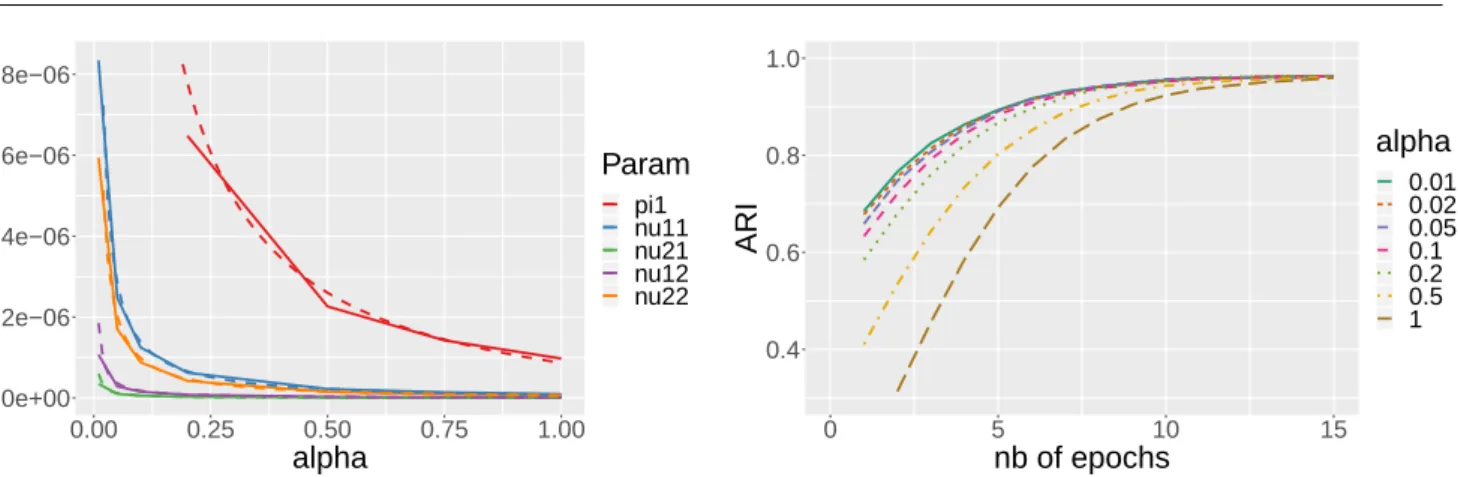
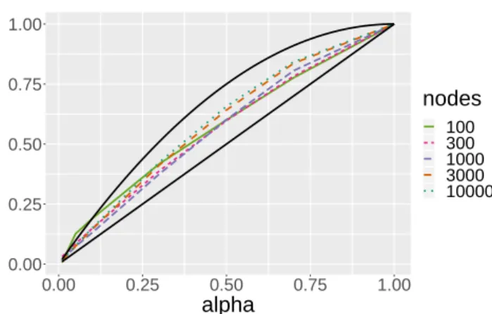
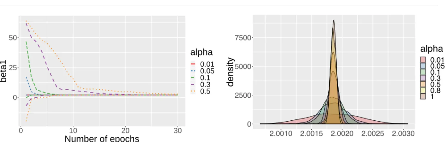
We will show that, provided the decreasing step sequence and the constant pseudo-step T are consistent, this allows for a significant speeding-up of the procedure (as well as

An implicit solver, based on a transport equation of void fraction coupled with the Navier-Stokes equations is proposed.. Specific treatment of cavitation source

References

Allassonni`ere S, Amit Y, Trouv´e A (2007) Toward a coherent statistical framework for dense deformable template estimation. J Roy Statist Soc Ser B 69:3–29 Allassonni`ere S, Kuhn E, Trouv´e A (2010) Construc-tion of Bayesian deformable models via a stochas-tic approximation algorithm: A convergence study. Bernoulli 16(3):641–678
Andrieu C, Moulines E, Priouret P (2005) Stability of stochastic approximation under verifiable conditions. SIAM J Control Optim 44(1):283–312
Capp´e O (2011) Online EM algorithm for hidden Markov models. Journal Computational and Graph-ical Statistics 20(3):728–749
Capp´e O, Moulines E (2009) On-line expectation-maximization algorithm for latent data models. J Roy Statist Soc Ser B 71(3):593–613
Davidian M, Giltinan DM (1995) Nonlinear Mod-els for Repeated Measurement Data. Chapman & Hall/CRC Press
(17)
Delyon B, Lavielle M, Moulines E (1999) Convergence of a stochastic approximation version of the EM al-gorithm. Ann Statist 27(1):94–128
Dempster AP, Laird NM, Rubin DB (1977) Maximum likelihood from incomplete data via the EM algo-rithm. J Roy Statist Soc Ser B 39(1):1–38
Duchateau L, Janssen P (2008) The frailty model. New York, NY: Springer
Fort G, Moulines E, Roberts GO, Rosenthal JS (2003) On the geometric ergodicity of hybrid samplers. Jour-nal of Applied Probability 40:123–146
Fort G, Jourdain B, Kuhn E, Leli`evre T, Stoltz G (2015) Convergence of the Wang-Landau algorithm. Mathematics of Computation 84(295):2297–2327 Hubert L, Arabie P (1985) Comparing partitions. J
Classif 2:193–218
Hull JJ (1994) A database for handwritten text recogni-tion research. IEEE Transacrecogni-tions on Pattern Analysis and Machine Intelligence 16(5):550–554
Karimi B, Lavielle M, Moulines E (2018) On the conver-gence properties of the mini-batch EM and MCEM algorithms, unpublished
Karimi B (2019) Non-Convex Optimization for Latent Data Models: Algorithms, Analysis and Applications. phD Thesis https://tel.archives-ouvertes.fr/ tel-02319140
Kuhn E, Lavielle M (2004) Coupling a stochastic ap-proximation version of EM with an MCMC proce-dure. ESAIM: P&S 8:115–131
Kuhn E, Lavielle M (2005) Maximum likelihood esti-mation in nonlinear mixed effects models. Comput Stat Data An 49(4):1020–1038
Lange K (1995) A gradient algorithm locally equiva-lent to the EM algorithm. J Roy Statist Soc Ser B 2(57):425–437
Liang P, Klein D (2009) Online EM for unsupervised models. In: Proceedings of Human Language Tech-nologies: The 2009 Annual Conference of the North American Chapter of the Association for Compu-tational Linguistics, Association for CompuCompu-tational Linguistics, NAACL ’09, pp 611–619
Matias C, Robin S (2014) Modeling heterogeneity in random graphs through latent space models: a selec-tive review. ESAIM: Proceedings and Surveys 47:55– 74
Neal RM, Hinton GE (1999) A view of the EM algo-rithm that justifies incremental, sparse, and other variants. In: Jordan MI (ed) Learning in Graphical Models, MIT Press, Cambridge, MA, USA, pp 355– 368
Nguyen H, Forbes F, McLachlan G (2020) Mini-batch learning of exponential family finite mixture models. Stat Comput.
Robert CP, Casella G (2004) Monte Carlo statisti-cal methods, 2nd edn. Springer Texts in Statistics, Springer-Verlag, New York
Titterington DM (1984) Recursive parameter estima-tion using incomplete data. J Roy Statist Soc Ser B 2(46):257–267
Figure
Fig. 1 Estimates of the parameter µ V using mini-batch MCMC-SAEM with α ∈ {0.1, 0.3, 0.5, 0.8, 1} as a function of the number of epochs.
Figure 2 presents for different values of the propor- propor-tion α the estimates of the empirical standard deviation with respect to the number of iterations
Fig. 4 Synthetic images sampled from the model for digit 5 using the parameter estimates obtained with the batch version on 20 images (top) and with the mini-batch version with α = 0.2 on 100 images (bottom).
Fig. 5 Estimation of the limit distribution of the estimate of ν 2,2 = 0.2 after 10 000 iterations for the mini-batch algorithm with proportions α ∈ {0.01, 0.05, 0.1, 0.2, 0.5, 0.75, 1}.
+4
Références
Documents relatifs