HAL Id: hal-02360465
https://hal.archives-ouvertes.fr/hal-02360465
Submitted on 12 Nov 2019
HAL is a multi-disciplinary open access
archive for the deposit and dissemination of
sci-entific research documents, whether they are
pub-lished or not. The documents may come from
teaching and research institutions in France or
abroad, or from public or private research centers.
L’archive ouverte pluridisciplinaire HAL, est
destinée au dépôt et à la diffusion de documents
scientifiques de niveau recherche, publiés ou non,
émanant des établissements d’enseignement et de
recherche français ou étrangers, des laboratoires
publics ou privés.
Distributed under a Creative Commons Attribution| 4.0 International License
The effect of crystal defects on 3D high resolution
diffraction peaks: a FFT-based method 3
Komlavi Eloh, Alain Jacques, Gabor Ribarik, Stéphane Berbenni
To cite this version:
Komlavi Eloh, Alain Jacques, Gabor Ribarik, Stéphane Berbenni. The effect of crystal defects on 3D
high resolution diffraction peaks: a FFT-based method 3. Materials, MDPI, 2018, 11 (9), pp.1669.
�10.3390/ma11091669�. �hal-02360465�
Materials 2018, 11, x; doi: FOR PEER REVIEW www.mdpi.com/journal/materials Article
1
The effect of crystal defects on 3D high resolution
2
diffraction peaks: a FFT-based method
3
K. Eloh1,2,3, A. Jacques1,3, *, G. Ribarik3,4, S. Berbenni2,3
4
1 Université de Lorraine, CNRS, IJL, F-54000 Nancy, France ; [email protected]
5
2 Université de Lorraine, CNRS, Arts et Métiers Paris Tech, LEM3, F-57000 Metz, France;
6
7
3Laboratory of Excellence on Design of Alloy Metals for low-mAss Structures (DAMAS), Université de
8
Lorraine, France.
9
4 Department of Materials Physics, Eötvös University, Budapest, Hungary.
10
* Correspondence: [email protected] ; Tel.: +03 72 74 26 79
11
Received: date; Accepted: date; Published: date
12
Abstract: Forward modeling of diffraction peaks is a potential way to compare the results of
13
theoretical mechanical simulations and experimental X-Ray Diffraction data recorded during in situ
14
experiments. As the input data are the strain or displacement field within a representative volume
15
of the material containing dislocations, a computer-aided efficient and accurate method to generate
16
these fields is necessary. With this aim, a current and promising numerical method is based on the
17
use of the Fast Fourier Transform (FFT) method. However, classic FFT-based methods present some
18
numerical artifacts due to the Gibbs phenomenon or ‘‘aliasing’’ and to ‘‘voxelization’’ effects. Here,
19
we propose several improvements: first, a consistent discrete Green operator to remove ‘’aliasing”
20
effects and second, a method to minimize the voxelization artifacts generated by dislocation loops
21
inclined with respect to the computational grid. Then we then show the effect of these
22
improvements on theoretical diffraction peaks.
23
Keywords: Dislocations; diffraction; FFT-based method; Discrete Green operator; voxelization
24
artifacts; sub-voxel method; simulated diffraction peaks; scattered Intensity
25
26
1. Introduction
27
X-Ray diffraction is one of the most powerful non-destructive tools to investigate materials, as
28
their wavelength is commensurate with the distance between atoms within a crystal [1–9]. Successive
29
improvements of both the X-Ray sources (from X-Ray tubes to third generation synchrotrons) and
30
detectors (from photographic plates and gas counters to fast two-dimensional arrays) have led to a
31
tremendous increase in the quantity of data recorded per unit time, allowing real time in situ or in
32
operando measurements [10,11]. It is now possible to determine the 3D grain microstructure of a bulk
33
material with a submicron resolution (using Topo-Tomography), to follow the evolution of the elastic
34
strain state of the grains of a polycrystal during mechanical tests (3D-XRD, far field diffractometry),
35
or to measure the distribution of strains within a few grains in real time (2D diffractometry)
36
[12,13].Such experiments result in terabytes of data recorded within a few days, which need to be
37
efficiently analyzed. In fact, only a low fraction of those data is actually treated because scientists lack
38
both time and software for further analysis [14].
39
The classical techniques used to analyze the 1D or 2D diffraction patterns recorded during tests
40
performed on polycrystalline specimens such as the Rietveld method, the square sines method to
41
measure internal stresses, or CMWP fitting for dislocations content often rely on simplified and
42
mathematically tractable models of a microstructure. Calculations which may involve simplifying
43
hypothesis lead to a general formula which can be used to fit one or several parameters of the
microstructure (dislocation densities and type, internal stress tensor…) to the diffraction pattern
45
(peak profiles, variation of the 2θ_B angle with orientation…)
46
During the last ten years, several authors proposed the opposite approach: forward modeling
47
[15–22]. This requires the design of a microstructure and the simulation of its behavior (often under
48
process or thermo-mechanical solicitation), the computation of the elastic strain field or the
49
displacement field. The last step is the generation through a ‘virtual diffractometer’ of a theoretical
50
diffraction pattern (different G vectors and different orientations of the lattice planes), which can be
51
compared with the experimental one. Depending on the size of the simulated representative
52
volume of matter and the experimental conditions such as the X-Ray beam coherence, different
53
assumptions can be done such as a coherent beam (where the amplitudes scattered by different points
54
add) or an incoherent beam (scattered intensities add), or for a partially coherent beam where a full
55
calculation may be necessary. Such modeling can be quite successful and can be used to validate the
56
different steps involved, mainly the microstructure and the constitutive law used to simulate the
57
material’s behavior.
58
However, as diffraction peaks contain information on different scales of a specimen: from
59
average quantities such as Type I (average) stresses related to the peaks’ positions, Type II (at grain
60
level) stresses related to its width, and Type III stresses (near the core of defects such as dislocations)
61
related to the peaks’ tails, a realistic simulation of a diffraction peak requires a description of a
62
material’s Representative Volume Element with a very fine mesh, i.e. a huge amount of CPU time
63
with classical methods used for simulations such as the Finite Element Method.
64
Numerical approaches based on the FFT for calculating the stress and strain fields within a
65
composite material received a surge of interest since the pioneering work of Moulinec and Suquet
66
[23,24]. They were first developed to compute effective properties and mechanical field of linear
67
elastic composites[23–26] and were extended to heterogeneous materials with eigenstrains
68
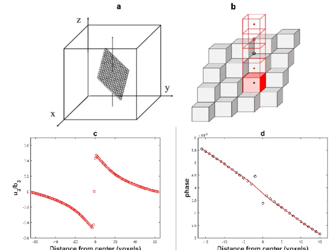
(dislocations, thermal strains…) [14,27–30]. They are also used for conductivity problems [31] ,
non-69
linear materials [25,27], viscoplastic or elastoviscoplastic polycrystals [32–36]. Today, FFT based
70
approaches represent alternative to finite element method because they are rather attractive in terms
71
of computation time [32].
72
However initial tests indicate that the displacement field computed (essential for diffraction
73
pattern generation) with FFT algorithms presents some numerical artifacts. These numerical artifacts
74
are due to Gibbs phenomenon or ‘‘aliasing’’ and to voxelization. The accuracy of the calculated strain
75
or displacement field is strongly influenced by these shortcomings and the simulated peaks may
76
provide wrong information on mechanical behavior or material characteristics. Therefore, it is
77
important to control these artifacts to simulate correct diffraction pattern in the case of a
78
microstructure containing different phases, grains, and crystal defects.
79
The aim of this paper is to improve the accuracy of the displacement field for diffraction peak
80
generation. This improvement is based on the introduction of a consistent discrete periodized Green
81
operator associated with the displacement field in order to take explicitly into account the
82
discreteness of the discrete Fourier Transform method [37]. The improvement of the voxelization in
83
FFT-method is performed through a sub-voxelization method will be described for inclined
84
dislocation loops. These improvements are reported and discussed. In the section 2, the FFT-based
85
method to compute the displacement field in a periodic medium is described. In section 3, the
86
treatment of voxelization problems in FFT-based approaches by a sub-voxelization method is
87
detailed in the case of slip plane not conforming to FFT grid. In the section 4, simulation of diffraction
88
peaks is reported and discussed.
89
2. Displacement field
90
2.1. FFT-based algorithm and mechanical fields
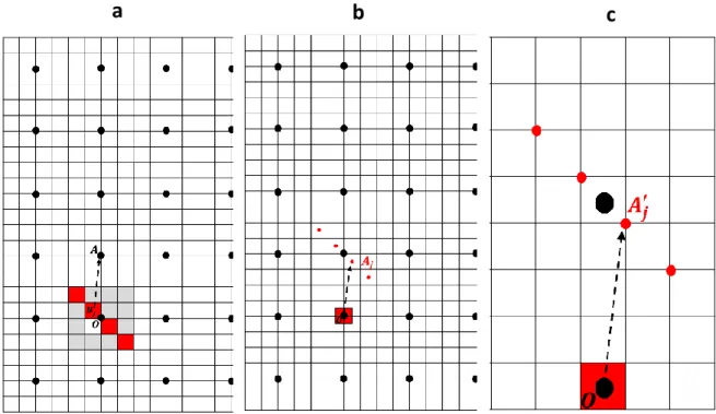
91
Let us consider a homogeneous elastic medium with eigenstrain assuming a periodic unit cell
92
discretized in 𝑁 × 𝑁 × 𝑁 voxels and subjected to an uniform overall strain tensor denoted 𝑬. Here,
93
this overall strain is the spatial average of the strain field in the unit cell (with external loading and a
given eigenstrain field). The unit cell contains dislocations (line defects) which are modeled with an
95
eigenstrain tensor. These dislocations create a displacement field during their motion along various
96
slip systems and thus generates strain/stress field [38].
97
The displacement vector is denoted 𝒖 and in the forthcoming equations, 𝒙 denotes any
98
position vector within the unit cell. All vectorial and tensorial fields will be written using bold
99
characters.
100
Starting from the equation for mechanical equilibrium, 𝑑𝑖𝑣 𝝈(𝒙) = 0 , and using elastic
101
equations, the displacement field is given at every positions by [39]:
102
𝒖(𝒙) = (𝑩 ∗ 𝒄𝟎: 𝛆∗)(𝒙) (1)
103
Where the symbol ∗ denotes the spatial convolution product, 𝒄𝟎 is the homogeneous linear elastic
104
stiffness, 𝜺∗ is the eigenstrain field and 𝑩 is a third order Green operator defined in Fourier space
105
as:106
𝐵̂ (𝝃) =𝑖𝑗𝑘 𝑖 2(𝐺̂ 𝜉𝑖𝑗 𝑘+ 𝐺̂ 𝜉𝑖𝑘 𝑗) (2)107
in which 𝑩̂ is the Fourier transform of 𝑩 and 𝑮̂ is the Fourier transform of the elastic Green
108
tensor [39]. Therefore, using the Fourier transform of spatial convolution product, Equation (1) can
109
be written in Fourier space as:
110
𝐮̂(𝛏) = 𝐁̂(𝛏): 𝐜𝟎: 𝛆̂ (𝛏) (3) ∗
111
Several numerical results showed that the use of the third order operator 𝑩̂ derived from the
112
classic Green 𝑮̂ leads to spurious oscillations on the computed displacement field near materials
113
discontinuities. The Discrete Fourier transform (DFT) used in this algorithm indeed transforms a
114
periodic function in real space into a periodic function in reciprocal space. However, the operator 𝑩̂
115
commonly used is the continuous analytic operator truncated to the size of the unit cell of the
116
reciprocal space: it is not periodic function. To fix this problem, we a periodized consistent discrete
117
Green operator using the DFT. The Fourier transform of this new operator 𝑩′̂ is written as function
118
of 𝑩̂ (the mathematical details about its derivation are given in [37]) and reads:
119
𝑩̂′(𝜉𝑖𝑗𝑘) = 𝐴𝑖𝑗𝑘 ∑ (−1)𝑚+𝑛+𝑝 (𝑚𝑁 + 𝑖) +∞ 𝑚,𝑛,𝑝=−∞ 1 (𝑛𝑁 + 𝑗) 1 (𝑝𝑁 + 𝑘)𝑩̂(𝜉𝑚𝑁+𝑖,𝑛𝑁+𝑗,𝑝𝑁+𝑘)120
With 𝐴𝑖𝑗𝑘= ( 𝑁 𝜋) 3 𝑠𝑖𝑛 (𝑖𝜋 𝑁) 𝑠𝑖𝑛 ( 𝑗𝜋 𝑁) 𝑠𝑖𝑛 ( 𝑘𝜋 𝑁) (4)121
Discrete frequency appearing in this equation is given when N is even by (T is the unit cell period):
122
𝝃 = (−𝑁 2+ 1) 1 𝑇, (− 𝑁 2+ 2) 1 𝑇, . . . , − 1 𝑇, 0, 1 𝑇, … . ( 𝑁 2− 1) 1 𝑇, ( 𝑁 2) 1 𝑇123
Here the sum on the 𝑩̂ operator is extended to the whole reciprocal space (in practice for 𝑚, 𝑛, 𝑝
124
up to a few tens) and folded up onto the unit cell of the DFT with suitable coefficients. The inverse
125
transform of 𝒖̂(𝝃) gives the displacement field at the center of each voxel.
126
We can also compute the displacement field at each voxel’s corner with a shifted operator using the
127
shift theorem:128
𝑩′ ̂′(𝜉 𝑖𝑗𝑘) = 𝐴𝑖𝑗𝑘𝑒𝑝𝜋 𝒊+𝒋+𝒌 𝑁 ∑ 1 (𝑚𝑁 + 𝑖) +∞ 𝑚,𝑛,𝑝=−∞ 1 (𝑛𝑁 + 𝑗) 1 (𝑝𝑁 + 𝑘)𝑩̂(𝜉𝑚𝑁+𝑖,𝑛𝑁+𝑗,𝑝𝑁+𝑘) (5)129
2.2. Numerical examples130
Let us consider a homogeneous material with isotropic elastic constant: Young’s modulus 𝐸 =
131
333.4 𝐺𝑃𝑎 and the Poisson ration 𝜗 = 0.26 . This approximately corresponds to the room
132
temperature elastic constants of single crystalline Ni-based Superalloys. The unit cell (Figure 1a) is
133
discretized in 128 × 128 × 128 voxels and contains a square-shaped inclusion discretized in
32 × 32 × 1 voxels corresponding to an Eshelby-like square prismatic loop perpendicular to the
z-135
axis. In order to generate a shift of the upper surface of the inclusion relative to its lower surface by a
136
Burgers vector 𝒃(0, 0, 𝑏3) the voxels within the inclusion are submitted to an eigenstrain: 𝜺𝑖𝑗∗ = 0
137
except 𝜺33∗ = 1 . We thus have 𝑏3= 𝑡 × 𝜺33∗ where 𝑡 the thickness of the inclusion in the
z-138
direction (i.e. the voxel size). This displacement field computed with the FFT algorithm using the
139
different periodized discrete Green operators is represented along z-axis in figure 1.
140
141
142
Figure 1: (a) Simulation of a squared dislocation in plane (001) by a platelet with eigenstrain; (b)
143
Component 𝑢3 of the displacement field (normalized by 𝑏3) along the z axis (arrow) computed with
144
the Green operator 𝑩 and showing oscillations; (c) Same component correct 𝑢3 computed with 𝑩′
145
The displacement at voxel (64,64,64) is zero in the center of the inclusion (c) and 𝑏3⁄ on its surface 2
146
(c). (d) Same component correct 𝑢3 computed with 𝑩′′.
147
When computed along a line crossing a dislocation loop, the displacement field exhibits a
148
discontinuity with a jump equal to Burgers vector 𝒃. This is indeed observed in figure 1. However,
149
the displacement field computed with the usual Green operator 𝑩 (figure 1b) also shows oscillations,
150
while which are not observed with the periodized operators 𝑩′ and 𝑩′′. An artificial damping of the
151
oscillations in figure 1b (such as a low pass filtering) might smooth these oscillations, but it would
152
also smooth the discontinuity.
153
2.3. Voxelization effect on the displacement field.
154
While the displacement field computed for dislocation loops having their planes parallel to the
155
faces of the simulated volume, artifacts appear for inclined loops, as shown in figure 2 for a
156
dislocation loop with a [01̅1] Burgers vector lying in a (111) slip plane of a fcc crystal. The
157
eigenstrain tensor is constrained in the region occupied by the dislocation loop (transformed voxels)
158
and is given by:
𝜀𝑖𝑗∗ = 𝐴𝑠
2𝑉(𝑛𝑖𝑏𝑗+ 𝑛𝑗𝑏𝑖) (6)
160
where 𝐴𝑠 is the area on which planes with normal 𝒏(𝑛1,𝑛2, 𝑛3) has slipped by a relative amount
161
𝒃(𝑏1,𝑏2, 𝑏3) and 𝑉 is the volume occupied by the loop [40,41]. As before, the dislocation loop is 32
162
voxels wide in the x and y directions, and 1 voxel thick but now with a z position such that 𝑥 + 𝑦 +
163
𝑧 = 𝑐𝑜𝑛𝑠𝑡𝑎𝑛𝑡. The displacement has been computed at the center of voxels with the periodized
164
operator 𝑩′ along z (figure 2b). As in figure 1c, the displacement in the center of a voxel belonging
165
to the loop plane (black dot in the reddish transformed voxel in figure 2b) is zero. The displacement
166
in the first neighboring voxels (red dot in figure 2b) are shifted relative to the expected position, so
167
that the displacement difference between these voxels is significantly lower than b, see figure 2c. It
168
can be checked in figure 2b that each of these voxels shares three faces with a transformed voxel. A
169
more detailed analysis shows that the second neighbors (which share three edges with transformed
170
voxels) are also slightly shifted in the opposite direction. The result is shown in figure 2d with: a
171
strong localized oscillation of the phase (taken here as the displacement modulo b).
172
Although the amplitude of this shift is small (less than 10% of the Burgers vector) it has
173
unwanted consequences on the diffraction peak simulation:
174
• The dislocation loops are surrounded by four impaired layers of voxels: As the scattered X-Ray
175
amplitude is proportional to the Fourier transform of G∙u (see equation (8) in section 4) we can
176
expect a phantom streak in the intensity in a direction perpendicular to the loop plane.
177
• The displacement field near the edges of the loop (near the dislocation line) will be quite different
178
from its expected value, and the strain field will not vary with the distance 𝑟 to the dislocation
179
line as 1 𝑟⁄ . This will strongly affect the tails of the diffraction peaks
180
181
182
Figure 2. (a) Modeling of a squared dislocation loop in a (111) plane as a layer of voxels with
183
eigenstrain; (b) position of the computed points relative to the transformed voxels with eigenstrains;
184
(c) Plot of the displacement field 𝑢3 (normalized by 𝑏3) along the z direction for dislocation loop
illustrated on figure 2. (d) Local oscillation of the phase due to the voxelization of the dislocation loop
186
(the representation is made for 32 voxels centered in the unit cell along z direction). The red line is
187
approximately equal to the phase expected for this displacement field.
188
3. Sub-voxelization method to correct voxelization effects.
189
3.1. Sub-voxelization method
190
The (conceptually) simplest way to remove this voxelization artifact would be to work on a
191
multiple grid (to multiply the number of voxels along each direction by 2, 4, or more), then to
192
downsample the displacement field data. In that case, FFT algorithms would lose much of their
193
interest due to these more demanding computational efforts. We show below that this can be done
194
in a more economical way by applying a patch to the FFT-computed displacement field. The basic
195
method is to compute on the same grid the difference vector:
196
∆𝑖(𝒙) = 𝑢𝑖𝑠𝑢𝑏(𝒙) − 𝑢𝑖ℎ𝑜𝑚(𝒙) (7)
197
where 𝑢𝑖𝑠𝑢𝑏(𝒙) is the displacement vector calculated for voxels where this eigenstrain is
198
concentrated on a single plane of sub voxels (figure 3b) and 𝑢𝑖ℎ𝑜𝑚 the displacement field in direction
199
i of voxels with a uniform eigenstrain (figure 3a). For the sake of clarity, we use 2D diagrams in Figure
200
3, but here the technique is applied to real 3D problems.
201
Figure 3. 2D representation of a dislocation loop in a tilted plane on a (8 × 8) FFT grid. (a) With a
202
homogeneous eigenstrain in the voxels occupied by the dislocation loop. (b) With each voxel
203
subdivided into 4*4 sub-voxels, only 4 of which are eigenstrained.
204
In order to compute the displacement due to sub-voxels, we use a 𝑁 × 𝑁 (𝑁 × 𝑁 × 𝑁) grid for
205
2D (resp. 3D) problems where each voxel can be subdivided into 𝑛 × 𝑛 (𝑛 × 𝑛 × 𝑛) sub voxels. Only
206
n (𝑛 × 𝑛) sub voxels are submitted to an eigenstrain field. At a point 𝑨 of the grid (black dots, figure
207
4a), we need to compute the sum of the displacements 𝒖𝒊𝒋 due to the n (𝑛 × 𝑛) sub voxels j (center
208
𝑩𝒋) within a voxel centered at point 𝑶. This sum is equivalent to the sum of the displacements due
209
to a strained sub voxel at point 𝑶 on the grid points 𝑨𝒋 such as 𝑶𝑨𝒋= 𝑩𝒋𝑨 (figure 4b). It is also
210
equivalent to the sum of the displacements 𝒖′𝒊𝒋 due to a full voxel at point 𝑶 on the initial grid on
211
points 𝑨′𝒋 such as 𝑶𝑨′𝒋= 𝑛𝑩𝒋𝑨 (figure 4c). The only difference between these last two sums is due to
212
the long-range strain field, and approximately results in a linear drift of the displacement. As the end
213
of the vectors 𝑶𝑨′𝒋 does not lie on the grid points (voxel centers) but on the corners of the voxels, the
214
𝒖′𝒊𝒋 displacements must be calculated with the shifted operator 𝑩′′ (equation (5)). A last point is the
215
scaling of the 𝒖𝒊 𝒋
and 𝒖′𝒊 𝒋
sums during the operations of figure 4. To keep the one Burgers vector
216
jump between both sides of the sub voxels plane in Figure 4a, the eigenstrain in the sub voxels must
217
be multiplied by n. The backwards change of scale requires a division by n: there is no scaling factor
218
between 𝑢𝑖ℎ𝑜𝑚 and 𝑢𝑖𝑠𝑢𝑏= ∑ 𝑢′𝑖 𝑗 .219
a
b
220
Figure 4. (a). 2D representation of the computational grid. Black dots correspond to the voxels center.
221
A voxel with center O is discretized in 4 × 4 in 2D (4 × 4 × 4 in 3D) sub-voxels. Some sub-voxels
222
contain an eigenstrain (red sub-voxels). We want to compute the displacement field at voxel centered
223
at point A, due to these deformed sub-voxels centered at 𝐵𝑗. (b) Effect of one deformed sub-voxel
224
centered at O on a row of sub-voxels centered at 𝐵𝑗 such as 𝑶𝑨𝒋= 𝑩𝒋𝑨. The sum of these effects is
225
equal to the previous displacement field. (c) Effect of deformed voxels centered at O on a row of voxels
226
(computed at corners 𝑨′𝒋 using Green operator 𝑩′′ ) such as 𝑶𝑨′𝒋= 𝑛𝑩𝒋𝑨 . This sum is equal to
227
previous wanted sum.
228
We need to compute ∆𝑖𝑗_𝑝𝑙(𝒙) the difference in displacement in direction i due to a voxel which
229
belongs to the plane “pl” (for fcc ‘’pl’’ is equal to (111), (1̅11), (11̅1), (111̅) ) of a dislocation loop
230
with a Burgers vector j at a position x relative to the transformed voxel. In practice, in a material with
231
cubic symmetry, it is sufficient to compute ∆13_(111)(𝒙) and ∆33_(111)(𝒙), and to use the symmetries
232
of the cube (fourfold [001] axis, threefold [111] axis, and (11̅0) symmetry plane) (and suitable
233
exchanges of the components of 𝒙) to obtain the required components. As it can be seen in figure 2b,
234
∆𝑖𝑗_𝑝𝑙(𝒙) is non-zero only for the neighbors of the transformed voxel, except the drift due to the long
235
range strain alluded above. The final recipe to compute ∆𝑖𝑗_𝑝𝑙(𝒙) and use the patch becomes:
236
• Compute the field 𝒄𝟎: 𝛆∗ defined in equation (1) for an isolated voxel with the eigenstrain
237
associated to a dislocation loop (equation (6)) with a Burgers vector [001] in a (111) plane (see
238
figure 2).
239
• Compute the displacement field in directions x(𝒖𝟏𝒉𝒐𝒎) and z (𝒖𝟑𝒉𝒐𝒎) at the voxels’ center around
240
the transformed voxel by convolution with the discrete periodized operator 𝑩′ (equation (4))
241
• Compute the displacement field in directions x and z at the voxels’ corners around the
242
transformed voxel by convolution with the shifted operator 𝑩′′ (equation (5))
243
• Calculate the 𝒖𝟏𝒔𝒖𝒃= ∑ 𝒖′𝟏
𝒋
and 𝒖𝟑𝒔𝒖𝒃= ∑ 𝒖′𝟑 𝒋
sums (𝑛 × 𝑛 terms for each sum) as in figure 4c,
244
then the raw ∆13(111)(𝒙) and ∆33_(111)(𝒙) for (𝑥1, 𝑥2, 𝑥3) going from -3 to 3 times the voxel size
245
t.
246
• Use the farthest voxels to correct the drift of the components so that all terms for large 𝒙 are
247
zero, and keep only the terms for the first three neighbors non zero. .
248
The patch can then be applied on the raw (FFT-based) displacement field by adding the
249
convolution of all transformed voxels of the different slip systems by the relevant ∆𝑖𝑗_𝑝𝑙(𝒙).
250
3.2. Results
251
For tests, we used the same 128 × 128 × 128 grid as above, and the transformed voxel was
252
divided into 8*8*8 sub voxels (using a reference medium with the same elastic constants as before).
253
Only the final values in units of b (after drift correction) of ∆13_(111)(𝒙) and ∆33_(111)(𝒙) are used
254
and others components are obtain by symmetries (Appendix A).
255
256
Figure 5. (a) Plot of the displacement field 𝑢3 (normalized by 𝑏3) along the z direction for dislocation
257
loop illustrated on figure2. Artifacts are removed by sub-voxel method described above. (b) the phase
258
(i.e. the displacement modulo a Burgers vector). With this correction, the phase is almost continuous.
259
The patch was used on the same configuration as in figure2. Figure 5a shows the resulting
260
displacement field and figure 5b the phase (i.e. the displacement modulo a Burgers vector) in Burgers
261
vector units. As it can be observed from figure 5a, the artifacts of the displacement field have
262
disappeared. In addition, the resulting phase varies smoothly even during the crossing of the
263
dislocation loop, see figure 5b.
264
4. Application on diffraction peak simulation
265
In this section, we show simulated diffraction peaks in order to point the effects of voxelization
266
artifacts and of the patch on numerical results. Under kinematical conditions and assuming a
267
coherent beam, the amplitude of a diffracted wave at a position 𝒒 in the vicinity of a reciprocal 𝑮
268
lattice vector is [14,18,42–44]:
269
𝐴(𝒒) = 𝐹𝑇[𝐴0(𝒓) × 𝐹(𝑮, 𝒙) × 𝑒𝑥𝑝 (−2𝑖𝜋 𝑮 ∙ 𝒖(𝒙))] (8)
270
where 𝒙 is the position of the scattering atom, 𝐴0(𝒙) is the amplitude of the incidence wave, 𝐹(𝑮, 𝒙)
271
is the local structure factor and 𝒖(𝒙) the displacement field. The scattered intensity is 𝐼(𝒒)= |𝐴(𝒒)|2.
272
For a face-centered cubic crystal, this intensity is non zero when G (h, k, l) is such as h, k, and l have
273
the same parity. Here two diffraction vectors G (200) and G (002) are used. They respectively
274
correspond to G∙b = 0 and G∙b = 1. The 3D diffracted intensity has been calculated using the FFT
275
instead of the continuous Fourier Transform, then summed in the planes perpendicular to the G
276
vector to obtain a linear plot along G equivalent to a I(2θ) plot. In figures 6a (G (200)) and 6c (G(002)),
277
we show the diffracted intensity (logarithmic scale) as a function of the pixel position 𝑖, and in figures
278
6b and 6d a logarithmic/logarithmic plot of the intensity vs. |𝑖 − 𝑖0| where 𝑖0 is the center of the
279
peak. In order to only study the effect of the displacement fields, we set A0(𝒙) = 1 and F(𝐆, 𝒙) = 1
280
for these simulations.
282
283
Figure 6. Simulated diffracted intensity as a function of the pixel position (logarithmic scale) . 3D
284
configuration is represented in 1D plot by making sum in each plane along an x-axis. Different way
285
for computing the displacement fields are studied for a dislocation loop with a [01̅1] Burgers vector
286
lying in a (111) slip plane . (a) Diffracted vector studied is G (200) corresponding to G∙b = 0. (b)
287
log/log representation of the intensity vs. |𝑖 − 𝑖0|. (c) and (d) Same as (a) et (b) but the studied
288
diffracted vector is G (002).
289
The peak shape near the top of the peaks is the same for both computing methods. It is perfectly
290
symmetric in the G∙b = 0 case and exhibits a bump on the right side for G∙b = 1. Their long-range
291
behavior is however quite different. When the displacement field has been calculated with the usual
292
truncated operator (black line), a phantom peak is observed at large |𝑖 − 𝑖0| (at large q), which is due
293
to the short period oscillations near the displacement field discontinuity (Figure 1a). The behavior of
294
the peak calculated with the modified Green operator (blue curve) is only slightly better: the intensity
295
at large q is underestimated in one case and overestimated in the other. When the intensity has been
296
calculated with the sub voxel patch (red curve) the long range intensity follows the expected
297
𝐼0|𝑖 − 𝑖0|−3 law [45,46]: the peak tails are indeed related to the highly distorted zones near the
298
dislocations’ cores. However, the red curve saturates at very large q. We suppose this is due to the
299
use of the Fast Fourier Transform instead of the continuous Fourier Transform in the calculation of
300
the scattered amplitude (equation (8)): The plot of figure 6 represents only one period in Fourier
301
space, and is repeated over and over on all Fourier space. We can now calculate the intensity of the
302
tails of these repetitions:
303
𝐼𝑛𝑒𝑖𝑏.= ∑ 𝐼0|𝑖 − 𝑖0− 128𝑚|−3 (9)
304
where m varies from -5 to 5 (zero excluded). We obtain the pink curve at the bottom of figures 5a and
305
5c. If we now plot the difference between the red intensity curve and this pink background line, we
306
obtain the green curve. On the log./log. plots, figure 6b and 6d it can be checked that this curve follows
307
the 𝐼0|𝑖 − 𝑖0|−3 law to the end. Thus, the residual error in the intensity computed by FFT results of
308
the FFT itself, and not from a residual error on the sub voxel corrected displacement field. If the
number of voxels is increased to 5123 or 10243 while keeping the physical size of the Representative
310
Volume constant this residual error should fall down to undetectable levels.
311
5. Conclusions
312
In this paper, we showed that although the use of a periodized Green operator in the FFT-based
313
method improves the final displacement field solution in a Representative Volume containing
314
discontinuities (dislocation loops), artifacts due to the voxelization of the dislocation loop planes are
315
still present with respect to analytical solutions. These artifacts have unwanted consequences on the
316
tails of diffraction peaks simulated by using this displacement field as input data.
317
We have introduced a patch which corrects these artifacts by simulating the displacement field
318
which would be obtained with a much finer voxelization without need to do the computations on a
319
finer grid. A simple construction method for this patch has been given and the patch can be used in
320
a single post-processing step to modify the initial FFT-based displacement field.
321
The modified displacement field has been used to simulate one-dimensional diffraction peaks.
322
The procedure strongly improves the shape of the peaks’ tails, i.e. it gives a good description of the
323
displacement field near the dislocation lines.
324
Acknowledgments: This work was supported by the French State through the program “Investment in the
325
future” operated by the National Research Agency (ANR) and referenced by ANR-11-LABX-0008-01
326
(LabEx DAMAS). Gabor Ribarik greatly acknowledge the support of the Janos Bolyai Research Fellowship
327
of the Hungarian Academy of Sciences.
328
Author Contributions: For the present paper, Komlavi S. Eloh performed the simulation work and wrote
329
the first draft of the paper; Alain Jacques analyzed numerical results and helped the simulation part; Gabor
330
Ribarik helped in constructing the computer code and helped in analyzing results; Stéphane Berbenni
331
helped in developing the first theoretical part of the paper. The paper was written by Komlavi S. Eloh,
332
Alain Jacques and Stéphane Berbenni.
333
Conflicts of Interest: The authors declare no conflict of interest.
334
Appendix A
335
∆𝟑𝟑_(𝟏𝟏𝟏)(𝒙𝟏, 𝒙𝟐, 𝒙𝟑) and ∆𝟏𝟑_(𝟏𝟏𝟏)(𝒙𝟏, 𝒙𝟐, 𝒙𝟑) have these symmetries due to the permutation
336
properties of the plan (𝟏𝟏𝟏)
337
∆33_(111)(𝑥1, 𝑥2, 𝑥3) = ∆33_(111)(𝑥2, 𝑥1, 𝑥3)338
∆33_(111)(𝑥1, 𝑥2, 𝑥3) = −∆33_(111)(−𝑥1, −𝑥2, −𝑥3)339
∆13_(111)(𝑥1, 𝑥2, 𝑥3) = −∆13_(111)(−𝑥1, −𝑥2, −𝑥3)340
The others values of ∆𝑖𝑗_(111)(𝒙) are given as function of ∆33_(111)(𝑥1, 𝑥2, 𝑥3) and ∆13_(111)(𝑥1, 𝑥2, 𝑥3):
341
∆11_(111)(𝑥1, 𝑥2, 𝑥3) = ∆33_(111)(𝑥3, 𝑥2, 𝑥1) ∆12_(111)(𝑥1, 𝑥2, 𝑥3) = ∆13_(111)(𝑥1, 𝑥3, 𝑥3)342
∆22_(111)(𝑥1, 𝑥2, 𝑥3) = ∆33_(111)(𝑥1, 𝑥3, 𝑥2) ∆31_(111)(𝑥1, 𝑥2, 𝑥3) = ∆13_(111)(𝑥3, 𝑥2, 𝑥1)343
∆32_(111)(𝑥1, 𝑥2, 𝑥3) = ∆13_(111)(𝑥3, 𝑥1, 𝑥2) ∆21_(111)(𝑥1, 𝑥2, 𝑥3) = ∆13_(111)(𝑥1, 𝑥3, 𝑥2)344
∆23_(111)(𝑥1, 𝑥2, 𝑥3) = ∆13_(111)(𝑥2, 𝑥1, 𝑥3)345
The value of ∆33(𝑥1, 𝑥2, 𝑥3) and ∆13(𝑥1, 𝑥2, 𝑥3) for the remaining plane (1̅11), (11̅1), (111̅) are
346
obtained using these symmetries:
347
∆33_(1̅11)(𝑥1, 𝑥2, 𝑥3) = ∆33_(111)(𝑥2, −𝑥1, 𝑥3) ∆13_(1̅11)(𝑥1, 𝑥2, 𝑥3) = ∆13_(111)(−𝑥1, 𝑥2, 𝑥3)348
∆33_(11̅1)(𝑥1, 𝑥2, 𝑥3) = ∆33_(111)(−𝑥2, 𝑥1, 𝑥3) ∆13_(11̅1)(𝑥1, 𝑥2, 𝑥3) = ∆13_(111)(𝑥1, −𝑥2, 𝑥3)349
∆33_(111̅)(𝑥1, 𝑥2, 𝑥3) = −∆33_(111)(𝑥2, 𝑥1, −𝑥3) ∆13_(111̅)(𝑥1, 𝑥2, 𝑥3) = −∆13_(111)(𝑥1, 𝑥2, −𝑥3)350
References351
1. Graverend, J.-B. L.; Dirand, L.; Jacques, A.; Cormier, J.; Ferry, O.; Schenk, T.; Gallerneau, F.; Kruch, S.;
352
Mendez, J. In Situ Measurement of the γ/γ′ Lattice Mismatch Evolution of a Nickel-Based Single-Crystal
353
Superalloy During Non-isothermal Very High-Temperature Creep Experiments. Metall and Mat Trans A
354
2012, 43, 3946–3951, doi:10.1007/s11661-012-1343-x.
355
2. Robinson, I.; Harder, R. Coherent X-ray diffraction imaging of strain at the nanoscale. Nat Mater 2009, 8,
356
291–298, doi:10.1038/nmat2400.
357
3. Pfeifer, M. A.; Williams, G. J.; Vartanyants, I. A.; Harder, R.; Robinson, I. K. Three-dimensional mapping of
358
a deformation field inside a nanocrystal. Nature 2006, 442, 63.
359
4. Ungár, T. Strain Broadening Caused by Dislocations Available online:
https://www.scientific.net/MSF.278-360
281.151 (accessed on Jun 16, 2018).
361
5. Ungár, T.; Gubicza, J.; Ribárik, G.; Borbély, A. Crystallite size distribution and dislocation structure
362
determined by diffraction profile analysis: principles and practical application to cubic and hexagonal
363
crystals. Journal of applied crystallography 2001, 34, 298–310.
364
6. Ribárik, G.; Ungár, T.; Gubicza, J. MWP-fit: a program for multiple whole-profile fitting of diffraction peak
365
profiles by ab initio theoretical functions. Journal of Applied Crystallography 2001, 34, 669–676.
366
7. Ribárik, G.; Gubicza, J.; Ungár, T. Correlation between strength and microstructure of ball-milled Al–Mg
367
alloys determined by X-ray diffraction. Materials science and engineering: A 2004, 387, 343–347.
368
8. Balogh, L.; Ribárik, G.; Ungár, T. Stacking faults and twin boundaries in fcc crystals determined by x-ray
369
diffraction profile analysis. Journal of applied physics 2006, 100, 023512.
370
9. Groma, I. X-ray line broadening due to an inhomogeneous dislocation distribution. Physical Review B 1998,
371
57, 7535.
372
10. Tréhorel, R.; Ribarik, G.; Schenk, T.; Jacques, A. Real time study of transients during high temperature creep
373
of a Ni-based superlloy by far field high energy synchrotron X-rays diffraction. Journal of applied
374
crystallography(under review).
375
11. Tréhorel, R. Comportement mécanique haute température du superalliage monocristallin AM1: Etude
in-376
situ par une nouvelle technique de diffraction en rayonnement synchrotron, Université de Lorraine: Nancy,
377
France, 2018.
378
12. Bernier, J. V.; Park, J.-S.; Pilchak, A. L.; Glavicic, M. G.; Miller, M. P. Measuring Stress Distributions in
Ti-379
6Al-4V Using Synchrotron X-Ray Diffraction. Metallurgical and Materials Transactions A 2008, 39, 3120–3133,
380
doi:10.1007/s11661-008-9639-6.
381
13. Miller, M. P.; Bernier, J. V.; Park, J.-S.; Kazimirov, A. Experimental measurement of lattice strain pole
382
figures using synchrotron x rays. Review of Scientific Instruments 2005, 76, 113903, doi:10.1063/1.2130668.
383
14. Jacques, A. From Modeling of Plasticity in Single-Crystal Superalloys to High-Resolution X-rays
Three-384
Crystal Diffractometer Peaks Simulation. Metallurgical and Materials Transactions A 2016, 47, 5783–5797,
385
doi:10.1007/s11661-016-3793-z.
386
15. Weisbrook, C. M.; Gopalaratnam, V. S.; Krawitz, A. D. Use of finite element modeling to interpret
387
diffraction peak broadening from elastic strain distributions. Materials Science and Engineering: A 1995, 201,
388
134–142, doi:10.1016/0921-5093(95)09757-0.
389
16. Miller, M. P.; Dawson, P. R. Understanding local deformation in metallic polycrystals using high energy
X-390
rays and finite elements. Current Opinion in Solid State & Materials Science 2014, 5, 286–299,
391
doi:10.1016/j.cossms.2014.09.001.
392
17. Demir, E.; Park, J.-S.; Miller, M. P.; Dawson, P. R. A computational framework for evaluating residual stress
393
distributions from diffraction-based lattice strain data. Computer Methods in Applied Mechanics and
394
Engineering 2013, 265, 120–135, doi:10.1016/j.cma.2013.06.002.
395
18. Vaxelaire, N.; Proudhon, H.; Labat, S.; Kirchlechner, C.; Keckes, J.; Jacques, V.; Ravy, S.; Forest, S.; Thomas,
396
O. Methodology for studying strain inhomogeneities in polycrystalline thin films during in situ thermal
397
loading using coherent x-ray diffraction. New J. Phys. 2010, 12, 035018, doi:10.1088/1367-2630/12/3/035018.
398
19. Song, X.; Xie, M.; Hofmann, F.; Illston, T.; Connolley, T.; Reinhard, C.; Atwood, R. C.; Connor, L.;
399
Drakopoulos, M.; Frampton, L. Residual stresses and microstructure in powder bed direct laser deposition
400
(PB DLD) samples. International Journal of Material Forming 2015, 8, 245–254.
401
20. Hofmann, F.; Song, X.; Jun, T.-S.; Abbey, B.; Peel, M.; Daniels, J.; Honkimäki, V.; Korsunsky, A. M. High
402
energy transmission micro-beam Laue synchrotron X-ray diffraction. Materials Letters 2010, 64, 1302–1305.
403
21. Hofmann, F.; Abbey, B.; Liu, W.; Xu, R.; Usher, B. F.; Balaur, E.; Liu, Y. X-ray micro-beam characterization
404
of lattice rotations and distortions due to an individual dislocation. Nature communications 2013, 4, 2774.
405
22. Suter, R. M.; Hennessy, D.; Xiao, C.; Lienert, U. Forward modeling method for microstructure
406
reconstruction using x-ray diffraction microscopy: Single-crystal verification. Review of Scientific Instruments
407
2006, 77, 123905, doi:10.1063/1.2400017.
408
23. Moulinec, H.; Suquet, P. A numerical method for computing the overall response of nonlinear composites
409
with complex microstructure. Computer Methods in Applied Mechanics and Engineering 1998, 157, 69–94,
410
doi:10.1016/S0045-7825(97)00218-1.
411
24. Moulinec, H.; Suquet, P. Fast numerical method for computing the linear and nonlinear properties of
412
composites. Comptes Rendus de l’Académie des Sciences. Série II 1994, 318.
413
25. Michel, J. C.; Moulinec, H.; Suquet, P. A computational scheme for linear and non-linear composites with
414
arbitrary phase contrast. International Journal for Numerical Methods in Engineering 2001, 52, 139–160.
415
26. Müller, W. Mathematical vs. Experimental Stress Analysis of Inhomogeneities in Solids. Journal de Physique
416
IV Colloque 1996, 06, C1-139-C1-148, doi:10.1051/jp4:1996114.
417
27. Vinogradov, V.; Milton, G. W. An accelerated FFT algorithm for thermoelastic and non-linear composites.
418
International Journal for Numerical Methods in Engineering 2008, 76, 1678–1695, doi:10.1002/nme.2375.
419
28. Anglin, B. S.; Lebensohn, R. A.; Rollett, A. D. Validation of a numerical method based on Fast Fourier
420
Transforms for heterogeneous thermoelastic materials by comparison with analytical solutions.
421
Computational Materials Science 2014, 209–217.
422
29. Graham, J. T.; Rollett, A. D.; LeSar, R. Fast Fourier transform discrete dislocation dynamics. Modelling Simul.
423
Mater. Sci. Eng. 2016, 24, 085005, doi:10.1088/0965-0393/24/8/085005.
424
30. Berbenni, S.; Taupin, V.; Djaka, K. S.; Fressengeas, C. A numerical spectral approach for solving
elasto-425
static field dislocation and g-disclination mechanics. International Journal of Solids and Structures 2014, 51,
426
4157–4175, doi:10.1016/j.ijsolstr.2014.08.009.
427
31. Eyre, D. J.; Milton, G. W. A fast numerical scheme for computing the response of composites using grid
428
refinement. Eur. Phys. J. AP 1999, 6, 41–47, doi:10.1051/epjap:1999150.
429
32. Prakash, A.; Lebensohn, R. A. Simulation of micromechanical behavior of polycrystals: finite elements
430
versus fast Fourier transforms. Modelling Simul. Mater. Sci. Eng. 2009, 17, 064010,
doi:10.1088/0965-431
0393/17/6/064010.
432
33. A. Lebensohn, R. N-site modeling of a 3D viscoplastic polycrystal using Fast Fourier Transform. Acta
433
Materialia 2001, 49, 2723–2737, doi:10.1016/S1359-6454(01)00172-0.
434
34. Lebensohn, R. A.; Rollett, A. D.; Suquet, P. Fast fourier transform-based modeling for the determination of
435
micromechanical fields in polycrystals. JOM 2011, 63, 13–18, doi:10.1007/s11837-011-0037-y.
436
35. Lebensohn, R. A.; Kanjarla, A. K.; Eisenlohr, P. An elasto-viscoplastic formulation based on fast Fourier
437
transforms for the prediction of micromechanical fields in polycrystalline materials. International Journal of
438
Plasticity 2012, 32–33, 59–69, doi:10.1016/j.ijplas.2011.12.005.
439
36. Suquet, P.; Moulinec, H.; Castelnau, O.; Montagnat, M.; Lahellec, N.; Grennerat, F.; Duval, P.; Brenner, R.
440
Multi-scale modeling of the mechanical behavior of polycrystalline ice under transient creep. Procedia
441
IUTAM 2012, 3, 76–90, doi:10.1016/j.piutam.2012.03.006.
442
37. Eloh, K. S.; Jacques, A.; Berbenni, S. Development of a new consistent discrete Green operator for
FFT-443
based methods to solve heterogeneous problems with eigenstrain. International Journal of
444
Plasticity(submitted) 2018.
445
38. Hirth, J. P.; Lothe, J. Theory of Dislocations; Krieger Publishing Company, 1982; ISBN 978-0-89464-617-1.
446
39. Mura, T. Micromechanics of Defects in Solids; Mechanics of Elastic and Inelastic Solids; 2nd ed.; Springer
447
Netherlands, 1987; ISBN 978-90-247-3256-2.
448
40. Li, Q.; Anderson, P. M. A Compact Solution for the Stress Field from a Cuboidal Region with a Uniform
449
Transformation Strain. Journal of Elasticity 2001, 64, 237–245, doi:10.1023/A:1015203721914.
450
41. Anderson, P. M. Crystal-based plasticity. Fundamentals of Metals Forming 1982, 277–279.
451
42. Takagi, S. A Dynamical Theory of Diffraction for a Distorted Crystal. Journal of the Physical Society of Japan
452
1969, 26, 1239–1253, doi:10.1143/JPSJ.26.1239.
453
43. Vartanyants, I. A.; Yefanov, O. M. Coherent X-ray Diffraction Imaging of Nanostructures. arXiv:1304.5335
454
[cond-mat] 2013.
455
44. Takagi, S. Dynamical theory of diffraction applicable to crystals with any kind of small distortion. Acta
456
Crystallographica 15, 1311–1312, doi:10.1107/S0365110X62003473.
457
45. Ungár, T. Microstructural parameters from X-ray diffraction peak broadening. Scripta Materialia 2004, 51,
458
777–781, doi:10.1016/j.scriptamat.2004.05.007.
459
46. Krivoglaz, M. A. Theory of X-Ray and Thermal Neutron Scattering by Real Crystals; Springer US, 1969;
460
ISBN 978-1-4899-5584-5.
461
© 2018 by the authors. Submitted for possible open access publication under the
462
terms and conditions of the Creative Commons Attribution (CC BY) license
463
(http://creativecommons.org/licenses/by/4.0/).


![[PDF] Guide de formation complet Python pour reviser | Cours informatique](data:image/gif;base64,R0lGODlhAQABAIAAAP///wAAACH5BAEAAAAALAAAAAABAAEAAAICRAEAOw==)