HAL Id: hal-00404718
https://hal.archives-ouvertes.fr/hal-00404718
Submitted on 17 Jul 2009
HAL is a multi-disciplinary open access
archive for the deposit and dissemination of
sci-entific research documents, whether they are
pub-lished or not. The documents may come from
teaching and research institutions in France or
abroad, or from public or private research centers.
L’archive ouverte pluridisciplinaire HAL, est
destinée au dépôt et à la diffusion de documents
scientifiques de niveau recherche, publiés ou non,
émanant des établissements d’enseignement et de
recherche français ou étrangers, des laboratoires
publics ou privés.
Sharp rates of decay of solutions to the nonlinear fast
diffusion equation via functional inequalities
Matteo Bonforte, Jean Dolbeault, Gabriele Grillo, Juan-Luis Vázquez
To cite this version:
Matteo Bonforte, Jean Dolbeault, Gabriele Grillo, Juan-Luis Vázquez. Sharp rates of decay of
solu-tions to the nonlinear fast diffusion equation via functional inequalities. Proceedings of the National
Academy of Sciences of the United States of America , National Academy of Sciences, 2010, 107 (38),
pp.16459-16464. �10.1073/pnas.1003972107�. �hal-00404718�
Sharp rates of decay of solutions to the nonlinear
fast diffusion equation via functional inequalities
M. Bonforte∗, J. Dolbeault†, G. Grillo‡, J. L. V´azquez∗§
∗Depto. de Matem´aticas, Universidad Aut´onoma de Madrid (UAM), Campus de Cantoblanco, 28049 Madrid, Spain,†Ceremade (UMR CNRS nr. 7534), Universit´e
Paris-Dau-phine, Place de Lattre de Tassigny, 75775 Paris 16, France,‡Dip. di Matematica, Politecnico di Torino, Corso Duca degli Abruzzi 24, 10129 Torino, Italy., and§ICMAT at UAM
The goal of this note is to state the optimal decay rate for solutions of the nonlinear fast diffusion equation and, in self-similar variables, the optimal convergence rates to Barenblatt self-similar profiles and their generalizations. It relies on the identification of the optimal constants in some related Hardy-Poincar´e inequalities and concludes a long series of papers devoted to generalized entropies, functional inequalities and rates for nonlinear diffusion equations.
Fast diffusion equation | porous media equation | Barenblatt solutions | Hardy-Poincar´e inequalities | large time behaviour | asymptotic expansion | interme-diate asymptotics | sharp rates | optimal constants
Introduction
The evolution equation ∂u
∂τ =∇ · (u
m−1
∇u) = m1 ∆um [ 1 ] with m6= 1 is a simple example of a nonlinear diffusion equa-tion which generalizes the heat equaequa-tion, and appears in a wide number of applications. Solutions differ from the linear case in many respects, notably concerning existence, regular-ity and large-time behaviour. We consider positive solutions u(τ, y) of this equation posed for τ ≥ 0 and y ∈ Rd, d
≥ 1. The parameter m can be any real number. The equation makes sense even in the limit case m = 0, where um/m has to be replaced by log u, and is formally parabolic for all m∈ R. No-tice that [ 1 ] is degenerate at the level u = 0 when m > 1 and singular when m < 1. We consider the initial-value problem with nonnegative datum u(τ = 0,·) = u0 ∈ L1loc(dx), where
dx denotes Lebesgue’s measure on Rd. Further assumptions
on u0 are needed and will be specified later.
The description of the asymptotic behaviour of the solu-tions of [ 1 ] as τ→ ∞ is a classical and very active subject. If m = 1, the convergence of solutions of the heat equation with u0 ∈ L1+(dx) to the Gaussian kernel (up to a mass factor) is
a cornerstone of the theory. In the case of equation [ 1 ] with m > 1, known in the literature as the porous medium equation, the study of asymptotic behaviour goes back to [1]. The result extends to the exponents m∈ (mc, 1) with mc := (d− 2)/d;
see [2]. In these results the Gaussian kernel is replaced by some special self-similar solutions UD,T known as the
Baren-blatt solutions (see [3]) given by UD,T(τ, y) := 1 R(τ )d “ D + 1−m 2 d |m−mc| ˛ ˛ y R(τ ) ˛ ˛2”−1−m1 + [ 2 ]
whenever m > mcand m6= 1, with
R(τ ) := (T + τ )d(m−mc )1 ,
where T≥ 0 and D > 0 are free parameters. To some extent, these solutions play the role of the fundamental solution of the linear diffusion equations, since limτ →0UD,0(τ, y) = M δ,
where δ is the Dirac delta distribution, and M depends on D. Notice that the Barenblatt solutions converge as m→ 1 to the fundamental solution of the heat equation, up to the mass factor M . The results of [1, 2] say that UD,T also describes
the large time asymptotics of the solutions of equation [ 1 ] as τ→ ∞ provided M =RRdu0dy is finite, a condition that
uniquely determines D = D(M ). Notice that in the range m≥ mc, solutions of [ 1 ] with u0∈ L1+(dx) exist globally in
time and mass is conserved:RRdu(τ, y) dy = M for any τ≥ 0.
On the other hand, when m < mc, a natural extension for
the Barenblatt functions can be achieved by considering the same expression [ 2 ], but a different form for R, that is
R(τ ) := (T− τ )−d(mc−m)1 .
The parameter T now denotes the extinction time, a new and important feature. The limit case m = mc is covered by
R(τ ) = eτ, U
D,T(τ, y) = e−d τ`D + e−2τ|y|2/d´−d/2. See
[4, 5] for more detailed considerations.
In this note, we shall focus our attention on the case m < 1 which has been much less studied. In this regime, [ 1 ] is known as the fast diffusion equation. We do not even need to assume m > 0. We shall summarize and extend a series of recent re-sults on the basin of attraction of the family of generalized Barenblatt solutions and establish the optimal rates of con-vergence of the solutions of [ 1 ] towards a unique attracting limit state in that family. To state such a result, it is more con-venient to rescale the flow and rewrite [ 1 ] in self-similar vari-ables by introducing for m6= mcthe time-dependent change
of variables t := 1−m2 log „ R(τ ) R(0) « and x :=q2 d |m−m1−m c| y R(τ ), [ 3 ] with R as above. If m = mc, we take t = τ /d and x =
e−τy/√d. In these new variables, the generalized Barenblatt
functions UD,T(τ, y) are transformed into generalized
Baren-blatt profilesVD(x), which are stationary:
VD(x) :=`D +|x|2´
1 m−1 x
∈ Rd. [ 4 ]
If u is a solution to [ 1 ], the function v(t, x) := R(τ )du(τ, y) solves the equation
∂v ∂t =∇ · » v∇ „vm−1 − Vm−1 D m− 1 «– t > 0 , x∈ Rd, [ 5 ] with initial condition v(t = 0, x) = v0(x) := R(0)−du0(y)
where x and y are related according to [ 3 ] with τ = 0. This nonlinear Fokker-Planck equation can also be written as
∂v ∂t = 1 m∆v m+ 2 1− m∇ · (x v) t > 0 , x∈ R d. Main results
Our main result is concerned with the sharp rate at which a solution v of the rescaled equation [ 5 ] converges to the gener-alized Barenblatt profileVDgiven by formula [ 4 ] in the whole
range m < 1. Convergence is measured in terms of the relative entropy given by the formula
E[v] :=m1 − 1 Z Rd » vm− Vm D m − V m−1 D (v− VD) – dx for all m 6= 0 (modified as mentioned for m = 0). In order to get such convergence we need the following assumptions on the initial datum v0 associated to [ 5 ]:
(H1) VD0≤ v0≤ VD1 for some D0> D1> 0,
(H2) if d ≥ 3 and m ≤ m∗, (v0− VD) is integrable for a
suitableD∈ [D1, D0].
The case m = m∗:= (d−4)/(d−2) will be discussed later.
Be-sides, if m > m∗, we define D as the unique value in [D1, D0]
such thatRRd(v0− VD) dx = 0.
Theorem 1. Under the above assumptions, if m < 1 and m6= m∗, the entropy decays according to
E[v(t, ·)] ≤ C e−2 Λ t
∀ t ≥ 0 . [ 6 ] The sharp decay rateΛ is equal to the best constant Λα,d> 0
in the Hardy–Poincar´e inequality of Theorem 2 with α := 1/(m− 1) < 0. Moreover, the constant C > 0 depends only onm, d, D0, D1, D andE[v0].
The precise meaning of what sharp rate means will be discussed at the end of this paper. As in [4], we can de-duce from Theorem 1 rates of convergence in more standard norms, namely, in Lq(dx) for q ≥ max{1, d (1 − m)/ [2 (2 − m) + d (1− m)]}, or in Ck by interpolation. Moreover, by
undoing the time-dependent change of variables [ 3 ], we can also deduce results on the intermediate asymptotics for the solution of equation [ 1 ]; to be precise, we can get rates of de-cay of u(τ, y)− R(τ )−dU
D,T(τ, y) as τ → +∞ if m ∈ [mc, 1),
or as τ→ T if m ∈ (−∞, mc).
It is worth spending some words on the basin of attrac-tion of the Barenblatt soluattrac-tions UD,T given by [ 2 ]. Such
profiles have two parameters: D corresponds to the mass while T has the meaning of the extinction time of the so-lution for m < mc and of a time-delay parameter otherwise.
Fix T and D, and consider first the case m∗< m < 1. The
basin of attraction of UD,T contains all solutions
correspond-ing to data which are trapped between two Barenblatt pro-files UD0,T(0,·), UD1,T(0,·) for the same value of T and such
that RRd[u0 − UD,T(0,·)] dy = 0 for some D ∈ [D1, D0]. If
m < m∗the basin of attraction of a Barenblatt solution
con-tains all solutions corresponding to data which, besides being trapped between UD0,T and UD1,T, are integrable
perturba-tions of UD,T(0,·).
Now, let us give an idea of the proof of Theorem 1. First assume that D = 1 (this entails no loss of generality). On Rd, we shall therefore consider the measure dµα:= hαdx,
where the weight hα is the Barenblatt profile, defined by
hα(x) := (1 +|x|2)α, with α = 1/(m− 1) < 0, and study
on the weighted space L2(dµα) the operator
Lα,d:=−h1−αdiv [ hα∇· ]
which is such thatRRdf (Lα,df ) dµα−1=RRd|∇f|2dµα. This
operator appears in the linearization of [ 5 ] if, at a formal level, we expand
v(t, x) = hα(x)
ˆ
1 + ε f (t, x) h1−mα (x)
˜ in terms of ε, small, and only keep the first order terms:
∂f
∂t +Lα,df = 0 .
The convergence result of Theorem 1 follows from the en-ergy analysis of this equation based on the Hardy-Poincar´e inequalities that are described below. Let us fix some nota-tions. For d≥ 3, let us define α∗:=−(d − 2)/2 corresponding
to m = m∗; two other exponents will appear in the
analy-sis, namely, m1 := (d− 1)/d with corresponding α1 = −d,
and m2 := d/(d + 2) with corresponding α2 =−(d + 2)/2.
We have m∗< mc < m2 < m1 < 1. Similar definitions for
d = 2 give m∗ = −∞ so that α∗ = 0, as well as mc = 0,
and m1 = m2 = 1/2. For the convenience of the reader, a
table summarizing the key values of the parameter m and the corresponding values of α is given in the Appendix.
Theorem 2. (Sharp Hardy-Poincar´e inequalities) Let d ≥ 3. For anyα∈ (−∞, 0) \ {α∗}, there is a positive constant Λα,d such
that Λα,d Z Rd|f| 2dµ α−1≤ Z Rd|∇f| 2dµ α ∀ f ∈ H1(dµα) [ 7 ]
under the additional condition RRdf dµα−1 = 0 if α < α∗.
Moreover, the sharp constantΛα,d is given by
Λα,d= 8 > > < > > : 1 4(d− 2 + 2 α) 2 if α ∈ˆ−d+2 2 , α∗ ´ ∪ (α∗, 0) , − 4 α − 2 d if α∈ˆ−d, −d+2 2 ´ , − 2 α if α∈ (−∞, −d) .
Ford = 2, inequality [ 7 ] holds for all α < 0, with the corre-sponding values of the best constantΛα,2= α2 forα∈ [−2, 0)
andΛα,2=−2α for α ∈ (−∞, −2). For d = 1, [7] holds, but
the values ofΛα,1 are given byΛα,1=−2 α if α < −1/2 and
Λα,1= (α− 1/2)2 ifα∈ [−1/2, 0).
The Hardy-Poincar´e inequalities [ 7 ] share many proper-ties with Hardy’s inequaliproper-ties, because of homogeneity rea-sons. A simple scaling argument indeed shows that
Λα,d Z Rd|f| 2(D + |x|2)α−1dx≤ Z Rd|∇f| 2(D + |x|2)αdx holds for any f ∈ H1((D +
|x|2)αdx) and any D
≥ 0, un-der the additional conditionsRRdf (D +|x|
2)α−1dx = 0 and
D > 0 if α < α∗. In other words, the optimal constant, Λα,d,
does not depend on D > 0 and the assumption D = 1 can be dropped without consequences. In the limit D→ 0, they yield weighted Hardy type inequalities, cf. [6, 7].
Theorem 2 has been proved in [4] for m < m∗. The main
improvement of this note compared to [8, 4] is that we are able to give the value of the sharp constants also in the range (m∗, 1). These constants are deduced from the spectrum of
the operatorLα,d, that we shall study below.
It is relatively easy to obtain the classical decay rates of the linear case in the limit m→ 1 by a careful rescaling such that weights become proportional to powers of the modified expression (1 + (1− m) |x|2)−1/(1−m). In the limit case, we
obtain the Poincar´e inequality for the Gaussian weight. As for the evolution equation, the time also has to be rescaled by a factor (1−m). We leave the details to the reader. See [9] for further considerations on associated functional inequalities.
A brief historical overview
The search for sharp decay rates in fast diffusion equations has been extremely active over the last three decades. Once plain convergence of the suitably rescaled flow towards an asymp-totic profile is established (cf. [1, 2] for m > mc and [4, 10]
for m≤ mc), getting the rates is the next step in the
asymp-totic analysis. An important progress was achieved by M.
Del Pino and J. Dolbeault in [11] by identifying sharp rates of decay for the relative entropy, that had been introduced earlier by J. Ralston and W.I. Newman in [12, 13]. The anal-ysis in [11] uses the optimal constants in Gagliardo-Nirenberg inequalities, and these constants are computed. J.A. Car-rillo and G. Toscani in [14] gave a proof of decay based on the entropy/entropy-production method of D. Bakry and M. Emery, and established an analogue of the Csisz´ar-Kullback inequality which allows to control the convergence in L1(dx),
in case m > 1. F. Otto then made the link with gradient flows with respect to the Wasserstein distance, see [15], and D. Cordero-Erausquin, B. Nazaret and C. Villani gave a proof of Gagliardo-Nirenberg inequalities using mass transportation techniques in [16].
The condition m≥ (d−1)/d =: m1was definitely a strong
limitation to these first approaches, except maybe for the entropy/entropy-production method. Gagliardo-Nirenberg inequalities degenerate into a critical Sobolev inequality for m = m1, while the displacement convexity condition requires
m ≥ m1. It was a puzzling question to understand what
was going on in the range mc < m < m1, and this has been
the subject of many contributions. Since one is interested in understanding the convergence towards Barenblatt profiles, a key issue is the integrability of these profiles and their mo-ments, in terms of m. To work with Wasserstein’s distance, it is crucial to have second moments bounded, which amounts to request m > d/(d + 2) =: m2 for the Barenblatt profiles. The
contribution of J. Denzler and R. McCann in [17, 18] enters in this context. Another, weaker, limitation appears when one only requires the integrability of the Barenblatt profiles, namely m > mc. Notice that the range [mc, 1) is also the
range for which L1(dx) initial data give rise to solutions which preserve the mass and globally exist, see for instance [1, 5].
It was therefore natural to investigate the range m ∈ (mc, 1) with entropy estimates. This has been done first by
linearizing around the Barenblatt profiles in [19, 20], and then a full proof for the nonlinear flow was done by J.A. Carrillo and J.L. V´azquez in [21]. A detailed account for these con-tributions and their motivations can be found in the survey paper [22]. Compared to classical approaches based on com-parison, as in the book [5], a major advantage of entropy tech-niques is that they combine very well with L1(dx) estimates
if m > mc, or relative mass estimates otherwise, see [4].
The picture for m ≤ mc turns out to be entirely
differ-ent and more complicated, and it was not considered until quite recently. First of all, many classes of solutions vanish in finite time, which is a striking property that forces us to change the concept of asymptotic behaviour from large-time behaviour to behaviour near the extinction time. On the other hand, L1(dx) solutions lose mass as time evolves. Moreover, the natural extensions of Barenblatt’s profiles make sense but these profiles have two novel properties: they vanish in finite time and they do not have finite mass.
There is a large variety of possible behaviours and many results have been achieved, such as the ones described in [5] for data which decay strongly as|x| → ∞. However, as long as one is interested in solutions converging towards Baren-blatt profiles in self-similar variables, there were some recent results on plain convergence: a paper of P. Daskalopoulos and N. Sesum, [10], using comparison techniques, and in two con-tributions involving the authors of this note, using relative entropy methods, see [8, 4]. This last approach proceeds fur-ther into the description of the convergence by identifying a suitable weighted linearization of the relative entropy. In the appropriate space, L2(dµ
α−1), with the notations of
Theo-rem 2, it gives rise to an exponential convergence after
rescal-ing. This justifies the heuristic computation which relates Theorems 1 and 2, and allows to identify the sharp rates of convergence. The point of this note is to explicitly state and prove such rates in the whole range m < 1.
Relative entropy and linearization
The strategy developed in [4] is based on the extension of the relative entropy of J. Ralston and W.I. Newmann, which can be written in terms of w = v/VD as F[w] :=1 1 − m Z Rd » w− 1 −m1`wm− 1´ – VDmdx .
For simplicity, assume m6= 0. Notice that F[w] = E[v]. Let I[w] := Z Rd ˛ ˛ ˛ ˛ 1 m− 1∇ ˆ (wm−1− 1) VDm−1˜ ˛ ˛ ˛ ˛ 2 v dx be the generalized relative Fisher information. If v is a solu-tion of [ 5 ], then
d
dtF[w(t, ·)] = − I[w(t, ·)] ∀ t > 0 [ 8 ] and, as a consequence, limt→+∞F[w(t, ·)] = 0 for all m < 1.
The method is based on Theorem 2 and uniform estimates that relate linear and nonlinear quantities. Following [4, 23] we can first estimate from below and above the entropyF in terms of its linearization, which appears in [ 7 ]:
hm−2 Z Rd|f| 2V2−m D dx≤ 2 F[w] ≤ h 2−mZ Rd|f| 2V2−m D dx [ 9 ] where f := (w− 1) Vm−1 D , h1(t) := infRdw(t,·), h2(t) :=
supRdw(t,·) and h := max{h2, 1/h1}. We notice that h(t) → 1
as t→ +∞. Similarly, the generalized Fisher information sat-isfies the bounds
Z Rd|∇f| 2V Ddx≤ [1 + X(h)] I[w] + Y (h) Z Rd|f| 2V2−m D dx [ 10 ] where h2(2−m)2 /h1 ≤ h5−2m =: 1 + X(h) and d (1− m) ˆ (h2/h1)2(2−m)− 1 ˜ ≤ d (1 − m)ˆh4(2−m) − 1˜=: Y (h). No-tice that X(1) = Y (1) = 0. Joining these inequalities with the Hardy-Poincar´e inequality of Theorem 2 gives
F[w] ≤h
2−m[1 + X(h)]
2ˆΛα,d− Y (h)˜ I[w]
[ 11 ] as soon as 0 < h < h∗:= min{h > 0 : Λα,d− Y (h) ≥ 0}. On
the other hand, uniform relative estimates hold, according to [23], formula (5.33): for some C = C(d, m, D, D0, D1),
0≤ h − 1 ≤ C Fd+2−(d+1)m1−m . [ 12 ]
Summarizing, we end up with a system of nonlinear differen-tial inequalities, with h as above and, at least for any t > t∗,
t∗> 0 large enough, d dtF[w(t, ·)] ≤ −2 Λα,d− Y (h) ˆ 1 + X(h)˜h2−mF[w(t, ·)] . [ 13 ]
Gronwall type estimates then show that lim sup
t→∞
e2 Λα,dtF[w(t, ·)] < +∞ .
This completes the proof of Theorem 1 for m6= 0. The adap-tation to the logarithmic nonlinearity is left to the reader. Results in [4] are improved in two ways: a time-dependent es-timate of h is used in place of h(0), and the precise expression of the rate is established. One can actually get a slightly more precise estimate by coupling [ 12 ] and [ 13 ].
Corollary 3. Under the assumptions of Theorem 1, if h(0) < h∗, then F[w(t, ·)] ≤ G`t, h(0),F[w(0, ·)]´ for any t ≥ 0,
whereG is the unique solution of the nonlinear ODE dG dt =−2 Λα,d− Y (h) [1 + X(h)] h2−mG with h = 1 + C G 1−m d+2−(d+1)m
and initial conditionG(0) =F[w(0, ·)].
Operator equivalence. The spectrum of
L
α,dAn important point of this note is the computation of the spectrum ofLα,dfor any α < 0. This spectrum was only
par-tially understood in [4, 8]. In particular, the existence of a spectral gap was established for all α6= α∗ = (2− d)/2, but
its value was not stated for all values of α.
J. Denzler and R.J. McCann in [17, 18] formally linearized the fast diffusion flow (considered as a gradient flow of the en-tropy with respect to the Wasserstein distance) in the frame-work of mass transportation, in order to guess the asymptotic behaviour of the solutions of [ 1 ]. This leads to a different functional setting, with a different linearized operator,Hα,d.
They performed the detailed analysis of its spectrum for all m∈ (mc, 1), but the justification of the nonlinear asymptotics
could not be completed due to the difficulties of the functional setting, especially in the very fast diffusion range.
Our approach is based on relative entropy estimates and the Hardy-Poincar´e inequalities of Theorem 2. The asymp-totics have readily been justified in [4]. The operatorLα,d=
−h1−αdiv [ hα∇· ] can be initially defined on D(Rd). To
con-struct a self-adjoint extension of such an operator, one can consider the quadratic form f 7→ (f, Lα,df ), where (· , · )
denotes the scalar product on L2(dµ
α−1). Standard results
show that such a quadratic form is closable, so that its clo-sure defines a unique self-adjoint operator, its Friedrich’s ex-tension, still denoted by the same symbol for brevity. The operatorHα,d is different: it is obtained by taking the
opera-tor closure ofLα,d, initially defined onD(Rd), in the Hilbert
space H1,∗(dµ α) := ˘ f∈ L2(dµ α−1) : R Rd|∇f|2dµα<∞ and R Rdf dµα−1= 0 if α < α∗ ¯ , so that Hα,df := h1−α∇ ·ˆhα∇`h1−α∇ · (hα∇f)´˜.
Because of the Hardy-Poincar´e inequality,RRd|∇f|
2dµ α
de-fines a norm. Denote byh · , · i the corresponding scalar prod-uct and notice thath f , g i = ( f , Lα,dg ) for any f, g∈ D(Rd).
Proposition 4. The operator Lα,d onL2(dµα−1) has the same
spectrum as the operators Hα,d onH1,∗(dµα).
The proof is based on the construction of a suitable unitary operator U : H1,∗(dµ
α) → L2(dµα−1), such that
UHα,dU−1 = Lα,d. We claim that U =
p
Lα,d is the
re-quested unitary operator. By definition, D(Rd) is a form
core of Lα,d, and as a consequence, the identity has to be
established only for functions f ∈ D(Rd). Since
kUfk2 = ` f ,Lα,df´=RRd|∇f| 2dµ α, we get ` UHα,dU−1f , g ´ =˙Hα,dU−1f , U−1g ¸ =`Lα,dU−1f ,Lα,dU−1g ´ =`U f , U g´=˙f , g¸ where we have used the properties U∗= U−1and U2=
Lα,d.
This unitary equivalence betweenLα,d andHα,d implies the
identity of their spectra.
We may now proceed with the presentation of the actual values of the spectrum by extending the results of [18]. Ac-cording to [24], the spectrum of the Laplace-Beltrami operator
on Sd−1 is described by
−∆Sd−1Yℓµ= ℓ (ℓ + d− 2) Yℓµ
with ℓ = 0, 1, 2, . . . and µ = 1, 2, . . . Mℓ:= (d+ℓ−3)! (d+2ℓ−2)ℓ! (d−2)!
with the convention M0 = 1, and M1 = 1 if d = 1. Using
spherical coordinates and separation of variables, the discrete spectrum ofLα,dis therefore made of the values of λ for which
v′′+“d−1 r + 2 α r 1+r2 ” v′+“ λ 1+r2− ℓ (ℓ+d−2) r2 ” v = 0 [ 14 ] has a solution on R+
∋ r, in the domain of Lα,d. The change
of variables v(r) = rℓw(−r2) allows to express w in terms of
the hypergeometric function2F1(a, b, c; z) with c = ℓ + d/2,
a + b + 1 = ℓ + α + d/2 and a b = (2 ℓ α + λ)/4, as the solution for s =−r2 of
s (1− s) y′′+ [ c− (a + b + 1) s ] y′− a b y = 0 , see [25]. Based on [8, 18], we can state the following result.
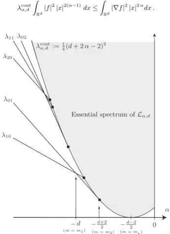
Proposition 5. The bottom of the continuous spectrum of the operatorLα,d onL2(dµα−1) is λcontα,d :=14(d + 2 α−2)
2.
More-over, Lα,d has some discrete spectrum only for m > m2 =
d/(d + 2). For d ≥ 2, the discrete spectrum is made of the eigenvalues λℓk=−2 α (ℓ + 2 k) − 4 k „ k + ℓ +d 2− 1 « [ 15 ] withℓ, k = 0, 1, . . . provided (ℓ, k)6= (0, 0) and ℓ + 2k − 1 < −(d + 2 α)/2. If d = 1, the discrete spectrum is made of the eigenvaluesλk= k (1− 2 α − k) with k ∈ N ∩ [1, 1/2 − α].
Using Persson’s characterization of the continuous spec-trum, see [26, 8], one can indeed prove that λcont
α,d is the optimal
constant in the following inequality: for any f∈ D(Rd
\ {0}), λcontα,d Z Rd|f| 2 |x|2(α−1)dx≤ Z Rd|∇f| 2 |x|2 αdx . λ01 λ10 λ11 λ02 λ20 Essential spectrum of Lα,d λcont α,d := 1 4(d + 2 α − 2) 2 − d −d+2 2 −d−22 α 0 (m = m1) (m = m2) (m = m ∗) Fig. 1.Spectrum ofLα,das a function ofα, ford = 5. 4
The condition that the solution of [ 14 ] is in the domain of Lα,ddetermines the eigenvalues. A more complete discussion
of this topic can be found in [18], which justifies the expression of the discrete spectrum.
Since α = 1/(m− 1), we may notice that for d ≥ 2, α = −d (corresponding to−2 α = λ10 = λ01=−4 α − 2 d) and α =
−(d+2)/2 (corresponding to λ01= λcont0 := 14(d+2 α−2) 2)
re-spectively mean m = m1= (d−1)/d and m = m2= d/(d+2).
The above spectral results hold exactly in the same form when d = 2, see [18]. Notice in particular that λcont
α,d=2 = α2
so that there is no equivalent of m∗for d = 2. With the
no-tations of Theorem 2, α∗= 0. All results of Theorem 1 hold
true under the sole assumption (H1).
In dimension d = 1, the spectral results are different, see [18]. The discrete spectrum is nonempty whenever α≤ −1/2, that is m≥ −1.
The critical case
Since the spectral gap of Lα,d tends to zero as m → m∗,
the previous strategy fails when m = m∗and one might
ex-pect a slower decay to equilibrium, sometimes referred as slow asymptotics. The following result has been proved in [23].
Theorem 6. Assume thatd≥ 3, let v be a solution of [5] with m = m∗, and suppose that (H1)-(H2) hold. If |v0− VD| is
bounded a.e. by a radialL1(dx) function, then there exists a positive constant C∗such that
E[v(t, ·)] ≤ C∗t−1/2 ∀ t ≥ 0 , [ 16 ] whereC∗depends only on m, d, D
0, D1, D andE[v0].
Rates of convergence in Lq(dx), q
∈ (1, ∞] follow. Notice that in dimension d = 3 and 4, we have respectively m∗=−1
and m∗= 0. In the last case, Theorem 6 applies to the
loga-rithmic diffusion.
The proof relies on identifying first the asymptotics of the linearized evolution. In this case, the bottom of the contin-uous spectrum of Lα∗,d is zero. This difficulty is overcome
by noticing that the operator Lα∗,d on R
d can be identified
with the Laplace-Beltrami operator for a suitable conformally flat metric on Rd, having positive Ricci curvature. Then the on-diagonal heat kernel of the linearized generator behaves like t−d/2 for small t and like t−1/2 for large t. The
Hardy-Poincar´e inequality is replaced by a weighted Nash inequality: there exists a positive continuous and monotone function N on R+such that for any nonnegative smooth function f with
M =RRdf dµ−d/2(recall that α∗− 1 = −d/2), 1 M2 Z Rd|f| 2dµ −d/2≤ N „ 1 M2 Z Rd|∇f| 2 dµ (2−d)/2 « . The function N behaves as follows: lims→0+s−1/3N (s) =
c1 > 0 and lims→∞s−d/(d+2)N (s) = c2 > 0. Only the first
limit matters for the asymptotic behaviour. Up to technicali-ties, inequality [ 13 ] is replaced by (F[w(t, ·)])3
≤ K I[w(t, ·)] for some K > 0, t≥ t0large enough, which allows to complete
the proof.
Faster convergence
A very natural issue is the question of improving the rates of convergence by imposing restrictions on the initial data. Re-sults of this nature have been observed in [19] in case of radi-ally symmetric solutions, and are carefully commented in [18]. By locating the center of mass at zero, we are able to give an answer, which amounts to kill the λ10mode, whose eigenspace
is generated by x7→ xi, i = 1, 2. . . d. This is an improvement
compared to the first result in this direction, which has been obtained by R. McCann and D. Slepˇcev in [27], since we obtain an improved sharp rate of convergence of the solution of [ 5 ], as a consequence of the following improved Hardy-Poincar´e inequality.
Lemma 1. Let eΛα,d:=−4 α − 2 d if α < −d and eΛα,d:= λcontα,d
ifα∈ [−d, −d/2). If d ≥ 2, for any α ∈ (−∞, −d), we have e Λα,d Z Rd|f| 2dµ α−1≤ Z Rd|∇f| 2dµ α ∀ f ∈ H1(dµα)
under the conditionsRRdf dµα−1 = 0 and
R
Rdx f dµα−1= 0.
The constant eΛα,d is sharp.
This covers the range m∈ (m1, 1) with m1= (d− 1)/d.
Theorem 7. Assume that m ∈ (m1, 1), d ≥ 3. Under
As-sumption (H1), if v is a solution of [ 5 ] with initial da-tum v0 such that RRdx v0dx = 0 and if D is chosen so that
R
Rd(v0− VD) dx = 0, then there exists a positive constant eC
depending only onm, d, D0, D1, D andE[v0] such that the
rel-ative entropy decays like
E[v(t, ·)] ≤ eC e− eΛα,dt ∀ t ≥ 0 .
A variational approach of sharpness
Recall that (d− 2)/d = mc< m1 = (d− 1)/d. The entropy
/ entropy production inequality obtained in [11] in the range m∈ [m1, 1) can be written asF ≤12I and it is known to be
sharp as a consequence of the optimality case in Gagliardo-Nirenberg inequalities. Moreover, equality is achieved if and only if v = VD. The inequality has been extended in [21] to
the range m∈ (mc, 1) using the Bakry-Emery method, with
the same constant 1/2, and again equality is achieved if and only if v = VD, but sharpness of 1/2 is not as straightforward
for m∈ (mc, m1) as it is for m ∈ [m1, 1). The question of
the optimality of the constant can be reformulated as a vari-ational problem, namely to identify the value of the positive constant
C = inf I[v] E[v]
where the infimum is taken over the set of all functions such that v∈ D(Rd) andR
Rdv dx = M . Rephrasing the sharpness
results, we know that C = 2 if m ∈ (m1, 1) and C ≥ 2 if
m∈ (mc, m1). By taking vn= VD(1 +n1f VD1−m) and letting
n→ ∞, we get lim n→∞ I[vn] E[vn] = R Rd|∇f| 2V Ddx R Rd|f|2V 2−m D dx .
With the optimal choice for f , the above limit is less or equal than 2. Since we already know thatC ≥ 2, this shows that C = 2 for any m > mc. It is quite enlightening to observe
that optimality in the quotient gives rise to indetermination since both numerator and denominator are equal to zero when v = VD. This also explains why it is the first order correction
which determines the value ofC, and, as a consequence, why the optimal constant,C = 2, is determined by the linearized problem.
When m≤ mc, the variational approach is less clear since
the problem has to be constrained by a uniform estimate. Proving that any minimizing sequence (vn)n∈N is such that
vn/VD− 1 converges, up to a rescaling factor, to a function f
associated to the Hardy-Poincar´e inequalities would be a sig-nificant step, except that one has to deal with compactness issues, test functions associated to the continuous spectrum and a uniform constraint.
Sharp rates of convergence and conjectures
In Theorem 1, we have obtained that the rate exp(−Λα,dt) is
sharp. The precise meaning of this claim is that Λα,d= lim inf h→0+ inf w∈Sh I[w] F[w],
where the infimum is taken on the setShof smooth,
nonneg-ative bounded functions w such thatkw − 1kL∞(dx)≤ h and
such that RRd(w− 1) VDdx is zero if d = 1, 2 and m < 1,
or if d ≥ 3 and m∗ < m < 1, and it is finite if d ≥ 3 and
m < m∗. Since, for a solution v(t, x) = w(t, x) VD(x) of
[ 5 ], [ 8 ] holds, by sharp rate we mean the best possible rate, which is uniform in t≥ 0. In other words, for any λ > Λα,d,
one can find some initial datum inShsuch that the estimate
F[w(t, ·)] ≤ F[w(0, ·)] exp(−λ t) is wrong for some t > 0. We did not prove that the rate exp(−Λα,dt) is globally sharp in the
sense that for some special initial data,F[w(t, ·)] decays ex-actly at this rate, or that lim inft→∞exp(Λα,dt)F[w(t, ·)] > 0,
which is possibly less restrictive.
However, if m ∈ (m1, 1), m1 = (d − 1)/d, then
exp(−Λα,dt) is also a globally sharp rate, in the sense that
the solution with initial datum u0(x) = VD(x + x0) for any
x0 ∈ Rd \ {0} is such that F[w(t, ·)] decays exactly like
exp(−Λα,dt). This formally answers the dilation-persistence
conjecture as formulated in [18]. The question is still open when m≤ m1.
Another interesting issue is to understand if improved rates, that is rates of the order of exp(−λℓkt) with (ℓ, k) 6=
(0, 0), (0, 1), (1, 0) are sharp or globally sharp under additional moment-like conditions on the initial data. It is also open to decide whether exp(−eΛα,dt) is sharp or globally sharp under
the extra conditionRRdx v0dx = 0.
Appendix. A table of correspondence
For the convenience of the reader, a table of definitions of the key values of m when d≥ 3 is provided below with the cor-respondence for the values of α = 1/(m− 1). This note is restricted to the case m∈ (−∞, 1), that is α ∈ (−∞, 0).
m = −∞ m∗ mc m2 m1 1 m = −∞ d−4 d−2 d−2 d d d+2 d−1 d 1 α = 0 −d−2 2 −d2 −d+22 −d −∞
ACKNOWLEDGMENTS. This work has been supported by the ANR-08-BLAN-0333-01 project CBDif-Fr and the exchange program of University Paris-Dauphine and Universidad Aut´onoma de Madrid. MB and JLV partially supported by Project MTM2008-06326-C02-01 (Spain). MB, GG and JLV partially supported by HI2008-0178 (Italy-Spain).
c
2009 by the authors. This paper may be reproduced, in its entirety, for non-commercial purposes.
1. Friedman, A. & Kamin, S. (1980) Trans. Amer. Math. Soc. 262, 551–563. 2. V´azquez, J. L. (2003) J. Evol. Equ. 3, 67–118. Dedicated to Philippe B´enilan. 3. Barenblatt, G. I. (1952) Akad. Nauk SSSR. Prikl. Mat. Meh. 16, 67–78.
4. Blanchet, A., Bonforte, M., Dolbeault, J., Grillo, G. & V´azquez, J. (2009) Archive for Rational Mechanics and Analysis 191, 347–385.
5. V´azquez, J. L. (2006) Smoothing and decay estimates for nonlinear diffusion equa-tions. Equations of porous medium type. (Oxford University Press, Oxford) Vol. 33, pp. xiv+234.
6. Caffarelli, L., Kohn, R. & Nirenberg, L., (1984) Compositio Math., 53, 259–275. 7. Hardy, G, Littlewood, J, & P´olya, G. (1934) Inequalities. (Cambridge University
Press).
8. Blanchet, A., Bonforte, M., Dolbeault, J., Grillo, G. & V´azquez, J.-L. (2007) Comptes Rendus Math´ematique 344, 431–436.
9. Bartier, J.-P., Blanchet, A., Dolbeault, J. & Escobedo, M. (2009) Improved interme-diate asymptotics for the heat equation. Preprint.
10. Daskalopoulos, P. & Sesum, N. (2008) J. Reine Angew. Math. 622, 95–119. 11. Del Pino, M. & Dolbeault, J. (2002) J. Math. Pures Appl. (9) 81, 847–875. 12. Newman, W. I. (1984) J. Math. Phys. 25, 3120–3123.
13. Ralston, J. (1984) J. Math. Phys. 25, 3124–3127.
14. Carrillo, J. A. & Toscani, G. (2000) Indiana Univ. Math. J. 49, 113–142.
15. Otto, F. (2001) Comm. Partial Differential Equations 26, 101–174.
16. Cordero-Erausquin, D., Nazaret, B., & Villani, C. (2004) Adv. Math. 182, 307–332. 17. Denzler, J. & McCann, R. J. (2003) Proc. Natl. Acad. Sci. USA 100, 6922–6925. 18. Denzler, J. & McCann, R. J. (2005) Arch. Ration. Mech. Anal. 175, 301–342. 19. Carrillo, J. A., Lederman, C., Markowich, P. A. & Toscani, G. (2002) Nonlinearity 15,
565–580.
20. Lederman, C. & Markowich, P. A. (2003) Comm. Partial Differential Equations 28, 301–332.
21. Carrillo, J. A. & V´azquez, J. L. (2003) Comm. Partial Differential Equations 28, 1023–1056.
22. Arnold, A., Carrillo, J. A., Desvillettes, L., Dolbeault, J., J¨ungel, A., Lederman, C., Markowich, P. A., Toscani, G. & Villani, C. (2004) Monatsh. Math. 142, 35–43. 23. Bonforte, M., Grillo, G. & V´azquez, J.-L. (2009, to appear) Archive for Rational
Mechanics and Analysis.
24. Berger, M., Gauduchon, P. & Mazet, E. (1971) Le spectre d’une vari´et´e riemannienne, Lecture Notes in Mathematics, Vol. 194. (Springer-Verlag, Berlin), pp. vii+251. 25. Weisstein, E. (2005) http://Mathworld.wolfram.com/HypergeometricFunctions.html. 26. Persson, A. (1960) Math. Scand. 8, 143–153.
27. McCann, R. J. & Slepˇcev, D. (2006) Int. Math. Res. Not. Art. ID 24947, p. 22.