Thermal emission of flat heating surfaces and ceiling heating panels with cylindrical heat sources

Publisher’s version / Version de l'éditeur:

Technical Translation (National Research Council of Canada), 1961

READ THESE TERMS AND CONDITIONS CAREFULLY BEFORE USING THIS WEBSITE.

https://nrc-publications.canada.ca/eng/copyright

Vous avez des questions? Nous pouvons vous aider. Pour communiquer directement avec un auteur, consultez la

première page de la revue dans laquelle son article a été publié afin de trouver ses coordonnées. Si vous n’arrivez pas à les repérer, communiquez avec nous à PublicationsArchive-ArchivesPublications@nrc-cnrc.gc.ca.

Questions? Contact the NRC Publications Archive team at

PublicationsArchive-ArchivesPublications@nrc-cnrc.gc.ca. If you wish to email the authors directly, please see the first page of the publication for their contact information.

Archives des publications du CNRC

For the publisher’s version, please access the DOI link below./ Pour consulter la version de l’éditeur, utilisez le lien DOI ci-dessous.

https://doi.org/10.4224/20331525

Access and use of this website and the material on it are subject to the Terms and Conditions set forth at Thermal emission of flat heating surfaces and ceiling heating panels with cylindrical heat sources

Kollmar, A.

https://publications-cnrc.canada.ca/fra/droits

L’accès à ce site Web et l’utilisation de son contenu sont assujettis aux conditions présentées dans le site LISEZ CES CONDITIONS ATTENTIVEMENT AVANT D’UTILISER CE SITE WEB.

NRC Publications Record / Notice d'Archives des publications de CNRC: https://nrc-publications.canada.ca/eng/view/object/?id=24d14f11-b49f-46ef-b4b1-ae0e539868ef https://publications-cnrc.canada.ca/fra/voir/objet/?id=24d14f11-b49f-46ef-b4b1-ae0e539868ef

Rad1ant heat1ng systems have several des1rab1e

features and have been 1n use for many years. Th1s

paper g1ves a cr1t1ca1 appra1sa1 of d1fferent methods of des1gn1ng a rad1ant heat1ng 1nsta11at10n and d1s-cusses some of the pract1ca1 problems wh1ch ar1se. It makes a s1gn1f1cant contr1but10n to th1s f1e1d of heat1ng technology, and has been translated 1nto

Eng11sh so that the mater1a1 w111 be more access1b1e. Most of the trans1at10n has been left 1n the l1tera1 Eng11sh equ1va1ent of the Germani but where th1s caused amb1gu1t1es the Eng11sh sentences have been rephrased.

The D1v1s10n 1s 1ndebted to Mr. D.A. S1nc1a1r of the Trans1at10ns Sect10n of the Nat10na1 Research Counc11 for prepar1ng th1s trans1at10n.

Ottawa,

January 1961

R.F. Legget, D1rector

Technlcal Translatlon 930

Tltle: Thermal emlsslon of flat heatlng surfaces and cel1lng

heatlng panels wlth cyllndrlcal heat sources

(WArmeabgabe von PlattenhelzflAchen und Helzdecken m1t zyllndr1schen wArmequellen)

Author: A. Kollmar

Reference: Gesundhe1ts-Ingen1eur, 80 (8): 225-235, 1959

Many klnds of flat heatlng surfaces, where the heat ls supplled

through internally sltuated pipes, are known in technology. They

are classlfled accordlng to whether the surface ln question ls thlck or thin and whether they are vertlcally or horizontally disposed relative to the heat duct. Most familiar in the flrst case ls the flnned pipe wlth round or quadrangular lamellae. The second type lncludes for example, cooklng plates with embedded electric heating cables (oven pipes, etc.). A larger field of application is found ln space heating with radiant heating plates and ceilings. Radlant heating plates are wide strips of sheet metal suspended below the

room ceiling and resting on heating pipes. The sheet metal is

joined to the pipes at the longitudinal axis by laminated or beaded

unions. In order to suppress the undesirable emission of heat on

the upper side of the plate an lnsulating layer of, for example,

glass bats ls applied here. The heat emisslon is thus predominantly by radiation. The theoretical calculatlon of the thermal emisslon from a radiant heatlng plate was successfully carried out on the basls of the thermal conduction ln the fin(l).

The heat transfer process within a heated cel1ing, wall or floor Can be represented in simplified form by a flat plate heated from a cylindrlcal heat source, assuming a temperature field that

ls constant in tlme. The storage of heat ls therefore not taken

into account. However, in road heating (snow melting installations) and floor heating systems lald directly on the ground, this heat retentlon in the dlrectlon of the ground interior can no longer be

left out of account. The opposite heat flow effect is found in the

artlflclal lce rink. In the latter case, if the ground is damp, a change ln the state of aggregation (freezing of the ground) ls added to the penetration of cold into the lnterlor of the ground, which is regarded as a body inflnltely extended in one directlon. Grlgull(2) has glven the theoretical principles of calculatlon

which, together with the following theory of temperature distribu-tion have made possible a practical method of calculating snow

melting installations(3) and artificial ice rinks(4). The

calcula-tion of ｴｨｾ heat emission from finned heating surfaces has been confined, in the known text books on heat ｴｲ｡ｮｳｦ･ｾ more or less to fins with rectangular or triangular cross-section (and also fins of very small material requirement according to E. Schmidt) and to

the round finned pipe. In the following section the well-known

rOd theory will be briefly reviewed. Raised Projection or Fin on a Plane

In the plane A, on which the raised fin (Fig. 1) is resting, let there be a uniform temperature t H and let the ambient tempera-ture be t L• The boundary surfaces .of the rod or fin are the heat-emitting ar6as F

O• In Fig. 1, if the thickness of the fin is very

small, e.g. in a convector or on a finned pipe, the frontal emission (plane 1) can be disregarded, i.e., q1

=

0 for x

=

h. The same

holds also for the infinitely extended rod (h ｾ 00), since here the

excess temperature t becomes zero (for simplicity let the ambient

temperature be zero). In the fin represented in Fig. 2a, q

=

0 for

x

=

h/2, because the temperature gradient between the pipes inside

the monolithic building material is zero at h/2. Only the last

two cases are mathematical boundary value requirements.

The differential equation for the temperature distribution in the rod and in the fin (Fig. 1) is, of course,

(1)

where m

］ｾ

with the heat transfer coefficient a assumed to be

constant in all directions, F

=

aL is the cross-section of the rod through which the heat passes at the foot of the raised projection

m

=

_ｾ

I

2a (a_haL+ L) _•

For a thin-walled fin or lamella, neglecting the small thick-ness a in the perimeter U,

m

=J

2a

A.a'

i.e., independent of the length L. If a piece of length L

=

I cut out from a thicker, but sufficiently long fin, so that on both sides in the longitudinal axis of the rib there is practically no tempera-ture effect, then the heat-emitting perimeter U

=

2L and the m-value

correspond to that of the thin-walled fin. The heat output of the rib of 1 m length without frontal heat emission is then, of course

or

= 2 (t _ t ) tanh (mh) [kcal

l

qRi a H L m mh

J .

( 5)

With frontal heat emission and the heat transfer coefficient aSn of this surface the equation becomes

a

*a

+ tanh(mh)

｛ｫｾｾｊＬｬ

1 + Sn tanh(mh)

J

rnA. or a Sn + tanh(mh) mA. a. m + Sn

x

｛ｫｾｾｉｊ

.

tanh (mh)

The literature also contains the equations for the temperature variation and the end fin temperature. _{The mean fin temperature t m} can be determined easily by equating the above expressions with the thermal emission of the fin surface given by qRi = _{nFO(tm - t L). It} can also be obtained from integration of the equation for the

tem-perature variation. For the fin Without heat emission we have

(8)

Rectangular Fin on a CIlinder in the Longitudinal Axis of the Latter

In the case of the fin of Fig. 2a and the plates of Fig. 2b to

d, the heat-generating surface is not flat but cylindrical. The

inner wall temperature of the heating pipe or the hot water tempera-ture ｾＧ is assumed constant (in view of the high numerical value of ai' the internal heat transfer resistance I/ni can be neglected

in the practical calculation). The stationary temperature field

thus depends on two coordinates. The two-dimensional potential theory to be applied in this case could now be carried over by the method of conformal mapping to the one-dimensional temperature dis-tribution of equation (1). Fig. 28: Fig. 2b: Fig. zc and d: (9) (10) (11)

The heat output of the pipe of 1 m length is obtained from

With the m-values of equation (10) and (11), 4a is to be re-placed in equation (12) by 2(a + x) and 2(X b + xc), respectively. For the plate of Fig. 2c and d we get, by subst1tution of the

2

m-valueand the numerical value of n , the equation

(13) The overall heat exchange coefficients x_{b and Xc are given by}

(14)

or with c₁ and the subscripts c, as the case may be. For the plate of Fig. 2b, Xc should be replaced in the above equation by ac. The x-values should be substituted when the plate thickness exceeds the

pipe diameter. Depending on the derivation, they apply to the upper or lower edge of the pipe (not to the middle of the pipe as stated erroneously in reference 5).

The specific heat output referred to 1 m2 upper (b) and lower (c) surface is obtained from

q _ qRo- } l (for equation 9) or _q

₌

_{qb + ｾ}

=

qRo_{h (for equation 10 and 11)}

｛Ｚｾｾｬｽ

Now, since qb

=

x b ｾ Xc (15a,b) (16a) or (16b) and hence (16C,d)

Equations 16 also hold for the distribution of the thermal emission qRo'

The mean surface temperatures t b and t c are obtainable from (17a) or

(for Fig. 2b again replace Xc by a c) or directly from

(17b)

X

t b

=

t_L + (t_H - t_L) b (18a)

[degr] • (18b)

Putting ｾ for the hyperbolic function divided by its argument, equation (18b) becomes

(Where the room air temperature differs above and below, see refer-ence 3, p.382, equ.(28l».

For Fig. 2b in equation (18b) Xc

=

a c

=

1. a_c a_c

NO\'l

(17C,d) From equations (17) or (18) it follows also that

tb - t L = OCr"b__

tc - tL OCb'"c

The infinite fin without thermal emission to the side (Fig. 3)

will now be considered as a special case. This would be possible

the arrangement of a row of pipes side by side, as in Fig. 4. The thermal emission to the environment then takes place only at the upper flat surface.

According to Fig. 3, for L

=

1 m, we have

or

｛ｾｾ｝

(19a)

(19b) By solving the two equations for the temperature differences, and adding the equations, we get

(20)

If an identical f1n is also present on the opposite side, then or, for different fin heights

(21)

where x'c is used by analogy with x'b' (The calculation can also be

carried out according to equations (11) and (12) with h/2

=

d/2.) For differing air temperatures t L and t A over and under the fin of Fig. 4, respectively,

Another special case is the single fin according to Fig. 5,

which emits heat in all directions. According to reference 5, heat

conduction in the fin is q = ａｏｾ､Ｏ､ • dt/dx. A thin fin is

as-sumed where the frontal emission and the f1n thickness can be

neg-lected in the heat exchanging per1meter. Then q = 2adtxdx' The

m-value is therefore found from the equat10n

.

Ｉｾ

[1]

and the heat em1ss1on as

(24) Tak1ng 1nto account the th1ckness 6, w1th slmultaneous em1ss1on of heat from the frontal surface, then

and

m =

.I4a.

(d +15) ｛ｾ｝

r

An2t5d _m

{,25 }

(26)

where uSn 1s aga1n the heat transfer coeff1c1ent of the frontal sur-face. It must be real1zed, of course, that these equat10ns proceed from mathemat1cal der1vat1ons thnt have been slmpl1f1ed w1th1n per-miss1ble 11m1ts. The curved lines of heat flow and the orthogonal 1sotherms or1g1nat1ng from the p1pe have been rect111nearly trans-formed. The heat furn1shed by all flow channels 1s thereby reta1ned. The effects of th1s d1m1n1sh with 1ncreas1ng f1n dimens1ons.

Through the temperature d1str1but1on these effects also sUbsta.nt1ally affect the heat tra.nsfer coeff1c1ents wh1ch, however, can scarcely be calculated accurately.

Example of F1g. 2: Let the d1ameter of the heating p1pe be

d

=

0.02 m. Let the p1pe 1nterval be h

=

0.30 m. The mean heat1ng

temperature 1s assumed to be t

H

=

50°C and the a1r temperature t L

=

20°C. Let the p1pe be embedded in concrete with a heat con-ducti vi ty coefficient A= 1 kcal/mh degrees. The upper and lower heat transfer coeff1cients are put equal and given the value

u

=

6 kcal/m2h degrees. Furthermore in Fig. 2b let b

=

0.04 m Fig. 2c let b = 0.04 m, c = 0.03 m Fig. 2d let b 1 = c1 = 0.04 m, b2

=

0.05 with A

₌

0.8 kcal/mh degree b₃ = 0.02 m with A= 0.05 and c₂ = 0.01 wlth A

=

0.7.

Let the pipe diameter d

=

2 em,

6 = 1 mm. Let the thermal

The results of the calculations according to the equations of this section are contained in Table I. It is clea!' from this that the specific heat output of the pipe qRo (for constant pipe interval) and the specific heat outputs of the surfaces decrease with

increas-ing embeddincreas-ing depth of the pipes. The effects of differing heat

conduction resistances are also clearly eVident. If the thermal

emission decreases on one side owing to a greater resistance to heat

conduction, then it increases somewhat on the other side. Good

thermal insulation upwards probably reduces the total thennal emis-sion but not that of the lower side (ceiling heating), if the heating pipes are brought as close as possible to the ceiling surface.

An Example for Fig. 3 and 4. Respective.lX: Let d = 0.02 rn, hb

=

he = 0.04, ｾ

=

1 kcal/rnh degrees (concrete), a

=

6 kcal/rn2h degrees, t H

=

50°C and t L

=

20°C.

Thus according to equation (20), qRo = 7.2 kcal/h and q

=

qRo/0.02'= 360 kcal/m2h _{and 180 kcal/m}2h

on the respective sides of the two surfaces. (For an equal number of unclad pipes it would be necessary to attain 11.3 kcal/mh and 565 kcal/m2h, respectively.) If deposits are found between the pipes the thermal emission is re-duced by approximately 2/n, i.e., to the above value.

If we assume in place of the pipe a rectangular duct of the same thickness, the thermal emission becomes q

=

306 kcal/m2h.

This illustrates the improvement of heat transfer due to the

cylin-drical shape. It becomes effective, however, only if the thermal

conduction resistance in equation (20) is significant when added to the film heat transfer resistance. (The heat conduction resist-ance in the covering of the pipe is about 1/5 as great as in the

case of plane surfaces on both sides.) With metallic materials

having high thermal conduction coefficients very high heat transfer

coefficients, such as those of steam or hot water, are needed. For

transferring heat to the air this metallic plate surface is not really suitable.

An Example According to Fig. 5: the height h

=

5 em and the thickness

conduction coefficient of the sheet steel fin be ｾ

=

50 kC8l/mh degrees. The hot water temperature is assumed to be t_H

=

80°C and the air temperature t L

=

20°C. Let the heat transfer coefficient be n

=

10 kcal/m2h _{degrees. From equation (23) we thus obtain an}

m-value of 9 and from equation (24) the heat emission of the fin is found to be Q_Ri

=

1.12 kcal/h. With a fin thickness of 1 cm where n Sn is again 10 kcal/m2h degrees, taking the frontal heat emission into account, m = 3.5 (according to equation (25» and Q

Ri

=

1.9 kcal/h (according to equation (26», i.e., not much more than for the fin only 1 mm thick. By erecting three fins of 1 mm thiclmess on a pipe 1 cm long we obtain almost twice the heat emission for the fin

1 cm thick.

Special Engineering Prohlems

In the practical design of heated ceilings according to Fig. 2d the ｦｯｬｬｯ｜ｾｩｮｧ questions of an economic nature arise:

1. Does the thermal emission of the heating pipe, qRo' increase

continuously with increasing pipe interval h? If not, is there a

maximum after which output decreases or remains constant?

2. How large must the pipe interval h be in order to secure

the maximum heat output qRO for a given pipe diameter d? Or,

con.versely, what is the minimum pipe diameter for a given pipe interval?

3. Is there a most favourable ratio of pipe interval to pipe

diameter (h/d)? This question follows from question 2.

For the simple fin (With frontal heat emission) according to Fig. 1, Eckert indicated(6) that the limit for a favourable applica-tion of the fin is reached when the heat transfer resistance l/n is equal to the heat conduction resistance of a flat wall of half the thickness of the fin. The equation therefore reads l/n

=

｡ＯＲｾＮ

The result follows from differentiation of equation (7) with respect

to h, with the maximum at dq/dh

=

O. For the cases of Fig. 2, on

the other hand, there is no frontal heat emission since this re-quirement constituted a boundary condition of the differential equation.

The facts requ1red 1n order to answer the above quest10ns can be der1ved, after some cons1derat10n, d1rectly from ･ｾｶ｡ｴＱＰｮｳ (II),

(12) and (10). The shape of the hyperbo11c tangent curve or 1ts

table of numer1cal values(7} shows that the value of mh/2 tends

towards un1ty. The thermal em1ss1on of the heat1ng p1pe 1ncreases

cont1nuously accord1ng to equat10n (12) w1th 1ncreas1ng h, but at mh/2 > ＰｾＱＴ there 1s no further substant1al 1mprovement. Hence the max1mum thermal emiss10n of the heat1ng p1pe 1s attained for prac-t1cal purposes at mh/2

=

n, 1.e., for a tanh value of 0.996.

Accordingly, w1th equat10n (II) we ohta1n

(27)

2n

and hence h =

cr m

It 1s also ev1dent that the greater m 1s, the smaller does the

p1pe 1nterval her become. The m-value 1s determined essentially by

the thermal conduct1v1ty and also by the p1pe d1mens1on. W1th poor

thermal conduct1v1ty a predeterm1ned heat output can only be atta1n-ed by ratta1n-educ1ng the p1pe 1nterval or greatly increas1ng the p1pe

d1ameter.

FOr the f1n of F1g. 1 Eckert(6} has calculated the max1mum

thermal em1ss10n of the f1n heat1ng surface for a m1n1mum expend1ture

of mater1al. By d1fferent1at1ng equat10n (4) w1th respect to a,

where ah/a = ｾＯ｡Ｌ and ｾ can be assumed constant, he obta1ned from

dq/da

=

0 the follow1ng result, wh1ch can be sOlved numer1cally or

graph1cally:

ｾ

ｨｾ As

=

1.419.

As prev10usly shown, the numerical result 1s not a r1g1d value. Therefore, 1f we put 1.419"".[2, then h=Jiil. For the heated

ce111ng accord1ng to F1g. 2d, 1f we subst1tute the m-value accord1ng to equat10n (II) and put h/2 instead of h, we then obta1n the

already determined equation (27), taking into account the additional factor 2/n2 in the m-value (if;2/J2/n2

=

n).

Parodi(8) has reproduced Eckert's solution with Kalous'

m-value. His suggestion from this that the output per fin does not

decrease, but remains almost constant, conforms with the present

work. Contrary to his opinion, however, the output per m2 area

beyond the critical length becomes smaller even in the fin with

lateral thermal emission only (Fig. 6). (Eckert also derived his

equation from this one, i.e., equation (4).) According to

equation (15a,b) the specific heat output q in kcal/m2h _decreases

continuously with increasing pipe interval h and constant thermal

emission qRo or qRi as the case may be. The highest specific heat

output 1s obtained with a heated ceiling as in Fig. 4. It decreases

continuously with increasing pipe interval. Beyond the critical

point the curve merely becomes flatter and reaches zero only at infinity.

In all ｴｄｾｳ･ considerations the heat transfer cOefficients were

assumed to be constant. Actually, however, they decrease as the

value of h increases, because the mean surface temperature also

de-creases. The q-values therefore decrease still more and the qRo

values do not quite reach the theoretical level at a given pipe

interval. Furthermore, for radiant ceiling heating the economic

maximum of thermal emission by the heating pipe (except in the case

of boundary heat) is not of decisive importance. In radiant ceiling

heating the ceiling dimensions are given, i.e., they are entirely

independent of the pipe intervals. Hence, e;wept for the heating

pipe there is no additional consumption of but LdLrig material, as in

the case of the metal finned pipe. The heated ceiling area required,

and hence the pipe intervals, are fully determined by the

calcula-tion of heat consumpcalcula-tion. In certain instances, if the whole ceiling

area is not involved in supplying the heat requirement and meeting the phySiologically admissible ceiling temperature, larger pipe

intervals may be chosen. One must realize, however, that great

variations in the pipe intervals from room to room cause different heat storage and hence different heatins-up times, and this fact

may work to the detriment of the heating system. It has hp8n demon-strated qui te frequently, also that the heated par- t of the ceiling is preferably placed in the front half of the space, both for

tech-nical and physiological reasons. However, on account of the

tem-perature stresses in the ceiling plaster, if the copper pipes are embedded in it, excessively steep transitions from the heated area of the ceiling containing the pipes are to be avoided. It is ｡､ｾ

visable to employ larger pipe intervals for the last few pipes

towards the inside of the room. With smooth gypsum plaster (not

without the addition of white lime as a softener) over lime mortar plaster, it is advisable to impress coarse sackcloth into the smooth

plaster. At the ceiling perimeter, of course, the ceiling has to

be cut. The economic advantages of larger pipe intervals, and

hence lesser pipe consumption, are more evident in the field of floor heating.

Now, to answer question 2, it is necessary only to solve equation (27) for hand d, accordingly

(28) and

(29)

as well as the ratio in question 3

(30) For practical purposes what has already been said also holds

here. This can easily be proved mathematically from the example

for Fig. 2d. According to Table I, m

=

7.84, and according to

equation (27) therefore h

=

2 • 3.14/7.84

=

0.80 m. In equations

(12) and (13) tanh (mh/2)

=

1 according to the assumptions made. With x b

=

1.5 and Xc

=

4.55 as well as A

=

1 we get qRo

=

46.2 kcal/ mh, q

=

58 kcal/m2h, qb

=

14 kcal/m2h and qc

=

44 kcal/m2h (from

to be t b

=

22.5°C and t c

=

27.2°C. The pipe diameter in the

example mentioned is d = 0.02 m and the heat transfer coefficient a = 6 kcal/m2h _{degrees. It is eVident, bhe r-ef'or-e that the thermal}

emission qc of the ceiling is too small for practice. If we took a

pipe interval ｡｣｣ｯｲｮｩｮｾ to the example h

=

0.3 m, then a pipe dia-meter of 2.8 mm according to equation (29) would suffice for the

aforementioned heat outputs. Since this diameter would lead to

a high pressure loss, let us assume a copper pipe of 12 mm diameter.

For this we obtain h = 0.62 m. The short calculation confirms the

indication, often expressed already, that it is favourable to design ceiling heating with relatively small pipe diameters, embedding the pipes iri the ceiling plaster. If applicable, the plaster ceiling

should be insulated from the supporting ceiling with a layer of

thermal insulation (reed bats or similar insulating bats or plates). Through the smaller embedding depth necessary a good thermal emission q is attained underneath the heating pipes towards the ceiling

surface, as well as reduced thermal inertia due to the insulation and hence faster heating up of the heat-emitting ceiling surface. For not too small pipe intervals, also, there is a still favourable

specific heat output of the heating pipe qRo (in kcal/mh). In

this Case the pressure loss with 3/8 inch copper pipe is no greater

than with 1/2 inch steel pipe. The smaller water content of the

installation at constant hot water temperature permits a smaller temperature drop, which in turn has a favourable effect on the thermal emission.

Comparison with the Rydberg-Huber Method of Calculation

The Rydberg-Huber method of calculation(9) for radiant heating ceilings according to Fig. 2 was derived from the two-dimensional potential theory by applying the Laplace differential equation. A comparison with the method of ｣｡ｬ｣ｵｬｾｴｩｯｮ presented here on the basis of experimental results from two concrete heating slabs with heating pipes at intervals of 10 to 40 cm showed practically

identi-cal numeriidenti-cal values·for the surface temperatures and hence also for

(wi th G

agreement with the fin theory may also be expected. Huber equation for the thermal emission is

A

= x + x )

b c

and for the mean ceiling surface temperature

The

Bydberg-en)

(32)

or, by changing the indices accordinglyI for the sur-race temperature

t b• Equations (15) to (17) also continue to hold. Neglecting the usually small numerical value of (Sl + $2) in equation (31),

h and for

n

=

d

a (the pipe interval ｩｾ thus given as circumference with the pipe diameter da) equation (31) is transformed into

(33)

Thus the mean ceiling surface temperature becomes

(34)

and by changing the indices, also suitable for the surface tempera-ture t b• However, equation (33) is just the pipe heat penetration equation extending from the internal pipe wall outward, neglecting l/(o.idi) and with the external heat transfer coefficient

a.'

=

_{(xb + xc). At the perimeter of the pipe, under the influence} of differing thermal conduction and convection resistances, somewhat different wall temperatures occur in the !y and x directions, which

the value of (Sl + S2) takes into account. (The higher the

resist-ance the higher the temperature and vice versa.) As radiant

heating ceilings are generally designed in practice (with respect to embedment depth, thermal conductvity and pipe intervals), these

The and (36)

temperature differences at the pipe perimeter can generally be left out of account without causing any serious error.

The heat-emitting surface increases steadily according to

equation. (33), ,jus t as in the case of the fin, with increasing pipe

interval h

=

_{nda• Question 1 of the preceding section should be}

raised here, therefore, in order to determine whether the heat

emission of the heating pipe behaves in the same way with increasing pipe interval h in accordance with equation (33) as in the case of of equations (12) and (13). We can achieve our purpose even without differentiation if we consider the denominator of equation (33)

somewhat more closely. c , A. _{and r i are assumed to be} conscant and then the denominator becomes the sum of a logarithmic curve ann a hyperbola. _{The term l/(ct'ra ) becomes steadily smaller with} increas-ing r a and the logarithmic term gets steadily bigger. The point of intersection of the two curves is the value beyond which the in-creasing logarithmic term begins to determine the heat emission,

i.e., from here on the heat emission gets continuously smaller. By

equating both equations we get

In Ya,

1 Yi 1 ",' Ya

ＭＭＬｾＧ = ---- Or - -= I n

-(\; YtJ A. YtJ A. Yi

where l/r_a is an equilateral hyperbola. The graphical solution of the equation gives

A. 211A.

Ya= -,- or her= - - - - [m] (as)

(J< "b+"0 u

or also h cr

=

ｭＲｾ､Ｇ

In equation (31), therefore

ｾｮ

G

=

ｨｾｲＮ

ratio of critical intervals according to equations (27)

h

i _{s hcr(fin) - mn 2d.}cr(Ryd) _ 2

For the numerical values of the example associated with Fig. 2d h cr

=

2n 1/6.05

=

1.04, but according to equation (28) h

=

0.80 m. In Order to obtain the same h-value it would be necessary to use the value 4.1 instead of 3.14 in equation (27), which would cor-respond to a tanh value of 0.9995. In this connection, the

indications of equation (27) can be referred to. Over the critical length of hcr = 1.04 the thermal emission qRo according to the fin theory remains constant or even continues to increase slightly,

whereas in the Rydberg-Huber equation the thermal, emission decreases again from that point on. This could only be correct if the heating pipe in the ceiling shows a greater coverage with respect to the two heat-emitting surfaces than is shown by the critical radius r a according to equation (36). The consequence is then a small ceiling heat emission. Fig. 6 shows the thermal emission curves q find qRo according to the two methods of calculation for Fig. 2d with the

dimensions and physical values of the given example. It is evident

from Fig. 6, for the usual pipe intervals of ceiling and floor

heating systems, that both methods of calculation are suitable. In

the overall behaviour, however, only the fin theory is theoretically applicable for the ｴｾｾ･ｳ of design used in practice. It demands no physical assumptions whatsoever beyond those of other methods.

Moreover the fin theory is the simplest for practical calculation purposes (in this connection see 01 data sheets 58 and 59).

Boundary Heat Emission

So far we have considered of a larger heat-emitting area boundaries are not noticeable.

the heating plate or ceiling as part in which the effects of the ceiling

Bradtke(lO) was the first to attack the problem of boundary heat emission because he believed that

therein lay the discrepancy between his low heat emissions, cal-culated with small heat transfer coefficients, and the generally

higher heat emissions customarily found in practice. For the usual

radiant heating ceiling dimensions, however, the boundary heat emission does not generally attain the order of magnitude assumed by him.

In the literature the value employed for the boundary heat has been kept low and has not been increased even for more appropriate cases. The ｲｾ｡ｳｯｮ for this is the fact that in the theoretical determination certain assumptions have to be made which often may not correspond to the practical conditions.

Even the direction of air circulation affects the boundary heat

emission. Two different situations arise, depending on whether

heated air from the heated ceiling surface flows dovm the boundaries

or cooler air flows towards them. In the former case the boundaries

receive additional heat convectlvely so that their heat emission is

increased. Part of the heat, however, penetrates into the ceiling

and increases the heat storage. If cooler air flows to the

boundaries, on the other hand, the specific boundary heat em'-ss1on

increases. These influences are hard to estimate on account of the

difficulty of determining the heat transfer coefficients and flow

processes theoretically. It is known from measurements that for

narrow ceiling heating areas there is a certain improvement of the heat emission over and above the boundary emission.

If the problem of boundary heat emission is gone into rather thoroughly here, it is because Parod1(S) has recently broached it and also because a special method of calculation is given in the

techn1call1terature(ll). Let a be the length of the radiator in

the pipe direction, which is bounded by the width of the room, and let b be the radiator width, characterized by a pipe interval h. This quantity is genprally arbitrary unless the entire room has to be covered, but even then the radiator can often be accommodated by increasing the specific heat emission qn (kcal!m2h) of the ceiling. Thus the quantity a is measured from the outside pipe bend (at pipe centre) and b from centre to centre of the first and last pipe laps.

If the boundary heat be considered an enlargement of the heating

area, in the form F = (a + b) (b + h) with pipe interval h taken

account of, then Fig. 7a applies. Let the heat requirement be Q and

let qD be the specific heat emission of the heating surface without

boundaries. This gives F = Q/qn = abe Owing to the influence of

the boundary heat this yields the required radiator dimension bl _{, as}

JL-(a+h)h

b'= Ｎｾ ... _ - [m]

a+h

if a is to remain constant. In design, therefore, the radiator

width b that wou Ld be obtained from the area a • b , can b.- reduced because of the supplementary boundary heat gain to the dimension b'. Indirectly, therefore, a greater specific heat emission of the

area F' = ab' is obtained. It is given by

The number of pipe laps n is obtained from bl

=

_{(n - l)h. According}

to Fig. 7a the boundary heat is

Q =(a+b'+h)hqn ｛ｾ｣ｬＭｬ｡ｬ｝Ｎ

b(lI.lllldl\.v'( (;:59 )

Now let us represent the boundary heat qE' as in the literature in U

the form Q

=

F(qD + qE)

=

F(qD + qRo F)' where, 8.S before, the heat

emission of the individual pipe in the radiator (referred to the ceiling heat emission) is also assumed for the end pipe.

According to Fig. 7b, F :; ab and the perimeter U

=

2(a + b).

Further, the heat emission is qRo

=

qDh. Thus we obtain

2 __-a h b'=3n [Ill]

a+h

and qI from equation (38).

For Fig. 7b the boundary heat is found to be

Q =(a+b')hqn

[kcal].

b••nd"ry h (41)

The radiator width from equation (40) is somewhat greater than

that from equation (37) because, 8S Fig. 7b shows, the four COrners

are not taken into account.

However, the heat emission of the end pipe should not be

treated as for the individual pipe in the radiator; but the maximum

heat emission qRo for the pipe interval h ｾ 00 should be used, i.e.,

with tanh x

=

1, in accord Hith treatments made in the previous

section.

AccordinlZ to the Rydberg-HUber calculation method the highest

pipe interval. Bevond this. according to their theory, the heat

emission qRo ｾ 0, if h ｾ 00. In reality, however, qRo does not

cr decrease, but remains practically constant.

The general method or calculating ceiling heating and also the special method for boundary heat emission according to the

literature(3) is thus correct 1n theoretical assumption, but is

based on Kalous' m-value, which according to the literature(5) should

now be corrected. Furthermore, the boundary heat emission of the

end pipe was cut off at the temperature of the down-flowing air, since then the edge of the heating area is itself heated convective-ly. Some of this heat is of course returned to the room by

radiation.

We shall now discuss the method of calculating the boundary h eat described in the thirteenth edition of Rietscbel (11).

In the previous presentation·, using equation 9.35a(11) and Fig. 8 with the notation given there, we obtain

JL_(a+6.5 h) (h+LIb)

b' = qD [m]

a+0,5h

and q' again from equation (38).

The boundary heat (Fig. 8) becomes

(42)

(4.3)

with the added quantity Ab to be taken from Fig. 9.10(11).

The hatched strips in Fig •. 8 result from the extension of the kbhb

pipe bends on both sldes. We have Ab

=

ｾ

-

_{h, where kb and hb}

refer to the boundary strlps and h

b is set equal to 1 m. k and h

hold for the radiator area. The heat penetration coefficient k of the heated cel1ing is obtalned from equatlons (15a) and (33a) as

•

The changing of only one of dimenslons a and b of the radiator

ls mathematically easier and more favourable for draughting purposes.

k := kR/h. Since here b

=

nh for the radiator width, then at both the end pipe the boundary heat for h/2, referred to qD is aLr-e ady

implied. Accordingly, the boundary heat influence of An end pipe

hb h + lib

extends over "2

=

2 •

Thus the value of lib is a.lready referred to the heat emission

of pipe radiator qD. When referred to the end pipe alone

h_{b '} = (h + 1) (in m) was assumed. In the calculated example

accord-ing to Fig. 9.14 in "Rietschelll _{the value of lib is 8.5 em and hence}

h_b

=

h + b

=

0.3 + 0.085

=

0.385 m.

The critical pipe interval her (now denoted by h b') for the maximum output according to the Rydberg-Huber method on which the

calculation 1s based, is computed from equation (36) as h_{b '}

=

1.24 m.

Actually, however, the maximum output is already reached according to equation (28) at h

b ' ｾ 0.91 m and according to equation (13) is

constant at qRo

=

58 kcal/mh. According to equation (33)

(Rydberg-Huber) qRo = 64.5 kcal/mh. It is thus about ten pereent higher,

but decreases with h_b' < 1.24 m. Hence, as long as h_{b '} Z 1 + h

(in m) the calculation of the boundary heat by the Rydberg-Huber

equation is approximately correct. This will be the case for most

radiant heating ceilings. However, if h_{b '} ｾ 1 + h, then a smaller

boundar-y heat is obtained. As already mentioned, however , the

theoretical calculation of the boundary also depends on factors which

cannot be taken into account accurately. For example, for the

boundary strips we should expect a Lower- a value (in ｾ and xc).

Nor is the effect of the pipe bend considered with sufficient accuracy.

The h_b value, calculated from the critical pipe interval (not,

as according to reference 11, estimated at 1 m), is found from

(44)

(Owing to the quotient the heat distribution of the pipe goes

equation (44), in the numerator and denominator, equation (33) for the pipe heat emission (Rydberg-Huber), where in qR referred to the

h 0

pipe interval h of the ceiling da

=

n

and 1n qRo referred to the

her 2 X

boundary heat propagation hb' da = """"ii""""

= ')(

+ ')( - (according to

b c

equation (36», then

For the exact calculation we substitute this h

=

(h + ｾ｢Ｉ value in equations (42) and (43).

The same procedure applied to the fin theory in equations (11), (12) and (27) leads to

(46)

(47) em]

If the representation of equation (42) is retained, but is computed by equation (46), then

JL-(a+0,5h) h

qD ＴｮｾＧ

m!!-I

b'= \ 2

a+0,5h

(38)

The boundary heat (Fig. 8), referred to the heating area of the ceiling, is calculated from

Q [( 05h) h +0,5b'h] [kchal].

= qD a+ . (h)

ｨｬＵＢｾ｡ｲＱ

ｨＬＬｾｭＲ (48)

In order to test these equations their limiting cases should

be considered. These are illustrated in Fig. 9. For example, if

a

=

h this leads to a serpentine train of pipes (Fig. 9B) and for b

=

h a hairpin form (9C). For b = 0 the form of the pipe is

per-pendicular (Fig. 9D). The heat emission of the hairpin form is

Q

=

a(qRO + qRo ) in kcal/h. If this form is unbent and stretched,

to

imagine the bend of the pipe to be extended above and pipe from qRo

cr In Fig. lOa this would be on the line 1-2 on both sioes.

then for the straight pipe we get Q = 2aqR • (The slight added

°b

length from the curved section was not taken into account.) By

equating we get qRo = qRo which is not true, however, even though

b h

both equations, in themselves, are correct. In the previous equa-tions, therefore, putting b = 0, the heat emission of the pipe qR

°h and the pipe interval h (as an independent allowance) must vanish. From this it becomes clear that the effect of the pipe bend is not to be related to the pipe interval h, but to h_b, as in the case of

the boundary pipe. Fig. 10 illustrates this behaviour. It shows

the idealized thermal flux and temperature lines about the pipe bend and around the pipe cross-section perpendicular to the plane of the figure.

The extension of the pipe bend undertaken in Rietschel-Raiss(ll) as an addition to the width of the radiator (a + 0.5h) now becomes referred to the critical pipe interval hb of the fin theory.

From Fig. lOb and d it is evident that for the straight end pipe, with infinite pipe interval, the heat flux lines, when seen either from the upper or lower heat emitting surfaces, appear only

as straight lines (Fig. lOb). In the cross-section these heat

flux lines are upward and downward curving hyperbolas and the

iso-therms are ellipses (Fig. 10d). The behaviour on the circular

be.nds of the radiator is illustrated in Fie. lOa and c. Only by rotating the section line w _{with hw until hw}

=

her is the maximum heat emission qRo

c r obtained, even when guing beyond her. Compared with the free circular bend, ｴｨｾｲ･ｦｯｲ･Ｌ there occurs a certain

lateral reduction in the heat emission of the qRo •

h

(One must below. )

From boundary cOnsiderations (with linear heat flow lines) we obtain a thermal emission of the free and extended pipe bend of TT

2 hqRo ,and if pipe bends are adjacent to pipe bends, we obtain

-hq_BO • The result for the glven case, where there ls an interval c r

of 2h from one plpe bend centre to the next, must 11e somewhere between these t wo values. If we plot the glven h-values from h/2

n

to h cr agalnst the extended plpe bend 2 h, taklng lnto account the lnternal surface of the plpe bend (as a dlfference, on account of the radlator length a to the end of the pipe hend between the ex-tended plpe bend ｡ｾ､ curved one), and then put the resultlng area

1 n h2 h2

F = h_crh(-₂ + -) - --_{4 4}

=

h_{c r '}h' we obtaln hi

=

1 ?8h - ----_{.- 4h} The c r•

latter expresslon can be neglected because lt ls small.

Wlth (n - 1) bends ln the radlator, (n - 1) 1.28h

=

1.28b

becomes the length of pipe for the aLLowanoe; 1.e., O.64b on each

slde of the radiator. _{The value of hb can thus also be written} (O.64b) h_b

=

_{b(O.64hb). In equations} (47) and (48), therefore, we may substitute

for O.5h. Accord.ingly, for the determlnation of the boundary heat emission in the final equatlons read

(49 )

or

(50 )

or

In the limiting case b l

=

0, at a thermal emission of

1910 kcal/h, we obtain from equation (49) (and also (50» an

extended pipe length of about 41 rn , From equation (37) (Parodi" s

method) the result is 49.7 m. The latter would therefore be twenty

percent more pipe than necessary. Individual radiRtor connecting

pipes in the concrete ceiling and referred to the ceiling thermal

emission are taken into account by Q

=

ｌｱｮｾ in kcal/h, where L is

their stretched-out length. In the case of several connecting pipes

situated side by side we start with the given pipe interval and carry out the calculation for (n - 1) inside pipes according to

equation (2). Hence for one pipe (from the two half end pipes)

insert tanh (m

ｾＩ

=

1 in equation (12). In the latter two Cases

equations (15) and (16) apply. From these considerations it will

be realized that the boundary heat emission, contrary to Parodils oPinion(8), surely follows from the infinite Pipe interval case.

Example of Boundary ｈ･ｾｴ Emission

The calculation is carried out with the same values as in the previous examples according to Fig. 2d and Table I, but for the

ceiling heat emission it is assumed that qn

=

127 kcal/h. (According

to Table I that would already be the entire heat emission both

up-wards and downup-wards.) The mean hot water temperature must then be

increased from 50°C to 60°C. The pipe heat emission referred to

the heated ceiling is thus qRo = 127 • 0.3 = 38 kcal/mh, and

n

referred to the total heat transfer, qRo = qROn(l + Xb/X_c)

=

38 • 1.33

=

50.5 kcal/mh (maximum outputs 46.2 and 62 kcal/mh, r-espect t vely) •

The pipe interval is h

=

0.30 and pipe diameter d

=

0.02 m.

Let the heat requirement of a room be 1910 kcal/h. Without taking

into account the boundary heat the necessary ceiling heating area would be F

=

Q/qn

=

15 m2 which would be attained with radiator w1dths a = 5.0 - 3.75 - 2.5 m and the radiator lengths

b

=

3 - 4 - 6 m. _{Also let t H}

=

60°C, t L

=

20°C, m

=

7.94 m-1 , / 2 2

ｾ｢ = 0.083 m (Fig. 9.10 of reference 11). From equation (45) for the maximum heat emission according to the Rydberg-Huber method we get ｾ｢

=

0.086 m, and according to the fin theory we get ｾ｢

=

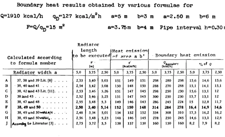
0.063m.

Table II contains the results of the calculations. It will

be seen that no essential differences in the percentage figures occur

except in line J. Methods A and B are based on an assumed constant

heat emission at the perimeter (Fig. 7) and between the pipes. This also accounts for its behaviour on changes of dimension when

the area of the radiator remains constant. It scarcely makes any

difference whether the heating slab is square or rectangular.

Never-theless the boundary heat emission of about 15% of the total emission

is noteworthy. In methods C to F the boundary heat is decreasing

if the radiator gets long and narrow (narrow with respect to width a), i.e., so that it has very many bends. (This is not favourable for the pressure drop in the radiator, either.) In the case of short wide radiators, the boundary heat attains the percentage values

shown in methods A and B. [It should be known that the boundary

heat will generally become a still higher percentage for small

total heating surface dimensions. However this is not always an

advantage from the standpoint of heat engineering, since for small heating areas there is generally also a low specific heat consump-tion (kcal/rn3h)]. With smaller pipe intervals (without changing the radiator dimensions a and b) the percentage of boundary heat de-creases going from A to E, althOUgh the heat emission of the radiator (in kcal/m2h) increases (Fig. 6).

The Rydberg-Huber method of calculation C (or D with the theoretical limiting value of the heat emission) and method E ac-cording to the fin theory, but in the form acac-cording to C, do not

differ appreciably. Method F gives in general somewhat higher

values than C, especially for short radiator widths. This is due to the pipe bend influence being considered too small in the case of C. Line G is obtained when n/4 is used in equations (49) and (50)

instead of 0.64. Then the pipe bend would be completely taken into

account with n/2 hqRO •

As already explained at the beginning of this section, method J must result in smaller values. But in all the methods, just as in the more exact theoretical ones, certain additional physical reduc-tions have to be expected, (smaller a values, temperature drop only to the temperature of the down-flowing air).

Concluding Remarks

For practical purposes we may recommend using the theoretically

most apt method F with equations (37), (4a) and (50)*. If one is

t_{H -} t _L'

very careful the approximate reduction factor t b

=

t _ t ' where

H L

t L is the air temperature of the room (e.go 20°C) and t L' the air temperature in the down draft at the he3ted ceiling as a function of the mean heated ceiling temperature (e.g. 25°C at t D = 41.2°C of the example), can be applied to the"hb value of these equations. For the given example this would be

t _{H -} t _L'

h • t = h = 0.363 60 - ｾｯｾ = 0.318

" b b b t

H - t L 60 - 2

Physically speaking, this temperature relation is attained when temperature differences that are assumed to be not exactly of the

same magnitude are used in the derivation of equation (46). Line G

of Table II contains the values thus obtained. If in the present

case the results do not in general reveal any great differences,

this is because in the calculation the h-value was 0.3 _{and h b}

=

0.386.

With smaller pipe intervals (e.g. h

=

0.15 m) a greater difference

occurs for the same m-value. In method A, ln this case, the

boundary heat becomes almost half too small, whereas for method F

it changes but little. This is immediately apparent when we

con-sider an area a • h of the same size according to Fig. 7a (method A). For large pipe interval h the specific heat emission (kcal!m2h)

becomes small and the boundary heat allowance becomes comparatively large. For small interval h the reverse holds. Actually, hOtiever,

•

The heat emission curves according to Fig. 11 and 12 of

the boundary heat does not decrease, but even increases somewhat. This is because the edge pipe cannot emit so much heat towards the inside (towards the other pipes) and its heat emission to the out-side therefore increases. The sum of both heat emissions, however, does not become as large as for the individual pipe. The greater

the pipe interval, the nearer we come to the sum value.

In conclusion it might be stated that the phySical value of· the boundary heat can probably be calculated more accurately than before, but still not to every detail of the heat exchange process.

References

[IJ Kollmar, A.: Die Berechnung einer Strahlplattenheizung. Heizg.• Liiftg., Haustechn. 3 (1952). S. 147.

[2JGrigull, U.:Groberj Erk. Die Grundgesetze der Warrneuber-tragung. 3. Auf!. BerlinfGottingenfHeidelberg 1955.

[3] Kollmar , A., u. Liese, W.: Die Strahlungsheizung. 4. Auf!. Miinchen 1957.

[4J Kollmar, A.: Berechnung des Kaltebedarfs einer Kunsteis-bahn. Ges.-Ing. 79 (1958), S. 266.

[5J Kollmar, A.: Die Warrncabgabe der Rohrdeckenheizung, Ges.-Ing. 80 (1959), S. 1.

[6J Eckert, E.: EinHihrung ill den Warrne- und Stoffaustausch. 2. Aufl. BerlinfGottingenfHeidelberg 1959.

[7J Ha-yashi, ]{.: Fiinfstellige Tafcln der Kreis- und Hyperbel-Iunktionen. Berlin 1941.

[8J Parodi, A.: Vom Aberglauben im Heizungs- und Liiftungs-fach. Heizg., Liiftg., lIaustechn. 9 (1958), S. 333.

[9J Rydberg,j. u. Huber,cs-:Varrncavgivning fran ror i betong eller mark. Stockholm 1955.

[10J Bradtke, F.: Abschn. Deckenheizung in "H. Rietschels Lehrbuch der Heiz- und Luftungstechnik". 12. Auf!. BerlinfGottingenfHeidelberg 1948.

[l1J RaifJ, W.: H. Rietschels Lehrbuch der Heiz- und Liiftungs-technik. 13. Auf!. BerlinfGottingenfHeidclberg 1958.

Table I

Calculations of an example for the heating plates of Fig. 2

---m t_b t _qRo q _{qb qc}

c

Fig.

1

°C °C kca1 kca1 kcaJ. kca1

m _{mh m}2h m2h m2h

--2a 11 36.8 36.8 60.6 202 101 101 2b 10.49 34.2 37.5 57 190 85 105 2c 10.05 34.6 35.4 54 180 87.5 92.5 2d 7.84 25.2 36 38 127 31 96

Table II

Boundary heat results obtained by various formulae for

Pipe interval h=O.30 m Q=1910 kcal/h qnr-127 kcal/m2h F=Qjq

_n

f:15 m2 Radiator a=5 m b=3 m a=3.15m b=4 m a=2.50 m b=6m

length ·He;:lt emif:si

0"1

Calculated according 1,-0 be executed ｾｦ ｾｲ･ｰ a b ' Boundary heat CPli.ssi.on

to formula number b' . g' _Qby..."ry

I

'I,of Q

[m) [kcal/m'b) [kcaIb)

Radiator tddth a 5,0 3,75 2,50 5,0 3,75 2,50

I

5,0 3,75 2,50 5,0 3,75 2,50 A 37, 38 lind 39 Lit. [8] . 2;53 3,40 5,05 151 149 151 298 280 298 15,6 14,6 15,6 B . 38, 40 and 41 2,54 3,42 5,08 150 148 150 288 270 288 15,1 14,1 15,1 C 38, 42 and 43 Lit. [11]. 2,53 3,46 5,26 151 147 145 298 250 230 15,6 13,1 12 D 38 and 45 . 2,52 3,46 5,25 151 147 145 300 250 230 15,7 13,1 12 E 38,47 and 48 2,55 3,48 5,3 149 146 143 286 245 224 15 12,8 11,7 F 38, 49 and 50 . 2,50 3,40 5,14 152 150 148 314 284 278 16,4 14,9 14,6 G 38, 49 and50"'\£11/4 . 2,48 3,34 5,01 154 152 152 334 308 310 17,5 16,2 16,2 H 38,49 lWld 50WJ4tJ.,•. 2,56 3,48 5,23 148 146 145 278 250 245 14,6 13,1 12,8 J ａｕＮｯｾ to Literatur [3] . 2,75 3,72 5,5 138 137 138 160 150 160 8,2 7,9 8,2

Fig. I

Raised fin on surface A

a fin thickness, h fin height, A thermal conductivity, L fin length

(1)

DC

ＭＭｾＬＺ

o

it.

Fig. 2

c and additional cylindrical heat conduits

equal to pipe thickness with floor made thicker on with different thicknesses Flat plates with

a heating plate

b heating plate

c heating plate

on both sides

d heated ceiling with plate as in

layers of structural material

one side of material

I tH I - l d r I he I I /

U

I 1 /I / / __...v Fig. 3

Fin on pipe axis without lateral heat emissions

_ _ _ _t'!_ _

t( (tA ) _

Fig. 4

" I T' I I I I - + j d H I I I I I I I I ) L_.J.' Fig. 5

Rectangular rod Or finite fin on pipe

fi 5 e 0,2 17,¥ D,G ae 1 2 J - P ' - p eｬＢｴ･ｬＧｖｾＧ hIm) Eq...",tionｊｊｻｒｹ､ｬｊ･ｲｧＭｈｵｾｲＩ 1-- --- - ---'--;-- -v- I-. l -r-, A ｴＴｾＢｴｩｯＢＬ 12 -/ N <,

1"-"

ｾＧｪ ｾ ＬＬｾ _ｩＧｾ f_ｾＧ＼ ｾＫ -Rllnge .1 _{｡ｰｰＢＧ｣ｾｴ［ｯＢ} fo'f" I---h ..ｾ N ce;,lin& 0,.ｾｉｾｯｲ ｨｾａｴ［ｮｾＭ ｾ ｾ［ _N ｾ ｾ 50 ｴｬｾ ｾ ':. "0 ｾ " ｾ 30 'i_.... ti 20

1

₀

1GO Fig. 6

Heat emissions as a function of the pipe interval according to

equations (33) (Rydberg-Huber) and (12) (fin theory) A Pipe emission qRo in kcal/mh

11/2 h/2 ｆﾷＨｯＮｾｨＩ Ｈ｢ｾｨＩ hlZ [ ] ] hi'

o

h/2 hlZ / I - + - ! Fig. 7

Boundary heat emission corresponding to equations (37) and (40)

(Methods A and B)

a radiator length, b radiator width, h pipe interval,

n number of laps of pipe

-1)h Z 0,,2511 aZ511 biZ! L ｾ

.

_{-- h,,/2} h/il -nil

ｾｨ

b=(n hl2i "1 h,,/ /Z-t _ｾｴ ｾ 0. 4 4b b*-F1g. 8

Boundary heat emiss10n corresponding to equation (42) (Method C)

a radiator length, b true radiator width, h pipe 1nterval,

n _{number of p1pe laps, h b} = Ab + h, b + hb = b* + Ab

=

b* + h + [Ab - h]. [Ab - h] contained in Rietschel-Ra1ss 13th ed.(ll),

o

®

o

Fig. 9

Radiator shapes for equal heat output Q[kca1/h] in limiting cases

A: Standard design, B: a

=

h,

c:

b = h, D: b

=

0

y

w

Fig. 10

Temperature level and heat flux lines

a at pipe bend, b on straight pipe, c perpendicular cutting plane