HAL Id: hal-01248140
https://hal.inria.fr/hal-01248140
Submitted on 8 Dec 2016
HAL is a multi-disciplinary open access
archive for the deposit and dissemination of
sci-entific research documents, whether they are
pub-lished or not. The documents may come from
teaching and research institutions in France or
abroad, or from public or private research centers.
L’archive ouverte pluridisciplinaire HAL, est
destinée au dépôt et à la diffusion de documents
scientifiques de niveau recherche, publiés ou non,
émanant des établissements d’enseignement et de
recherche français ou étrangers, des laboratoires
publics ou privés.
Stabilized Galerkin for transient advection of differential
forms
Holger Heumann, Ralf Hiptmair, Cecilia Pagliantini
To cite this version:
Holger Heumann, Ralf Hiptmair, Cecilia Pagliantini. Stabilized Galerkin for transient advection of
differential forms. Discrete and Continuous Dynamical Systems - Series S, American Institute of
Mathematical Sciences, 2016, 9 (1), pp.185 - 214. �10.3934/dcdss.2016.9.185�. �hal-01248140�
Volume X, Number 0X, XX 200X pp. X–XX
STABILIZED GALERKIN FOR TRANSIENT ADVECTION OF DIFFERENTIAL FORMS
Holger Heumann
EPI CASTOR, INRIA M´editerran´ee
2004 Route des Lucioles, Sophia Antipolis, France
Ralf Hiptmair and Cecilia Pagliantini
Seminar for Applied Mathematics, ETH Z¨urich
R¨amistrasse 101, Z¨urich, Switzerland
(Communicated by the associate editor name)
Abstract. We deal with the discretization of generalized transient advection problems for di↵erential forms on bounded spatial domains. We pursue an Eulerian method of lines approach with explicit timestepping. Concerning spatial discretization we extend the jump stabilized Galerkin discretization proposed in [H. Heumann and R. Hiptmair, Stabilized Galerkin methods for magnetic advection, Math. Modelling Numer. Analysis, 47 (2013), pp. 1713– 1732] to forms of any degree and, in particular, advection velocities that may have discontinuities resolved by the mesh. A rigorous a priori convergence theory is established for Lipschitz continuous velocities, conforming meshes and standard finite element spaces of discrete di↵erential forms. However, numerical experiments furnish evidence of the good performance of the new method also in the presence of jumps of the advection velocity.
1. Introduction. The equations of magneto-hydrodynamics (MHD) [16, Section 3.8], [22, Section 4.1] provide a consistent description of the interaction of elec-tromagnetic fields and conducting non-magnetic fluids like plasmas. The stan-dard model for resistive MHD under a quasi-neutrality assumption comprises bal-ance equations for mass, momentum and energy together with material laws and Maxwell’s equations in their magneto-quasistatic reduction (eddy current model) for the electromagnetic fields.
The traditional formulation of the linear eddy current model in the presence of a conducting fluid moving with velocity = (x, t) boils down to the evolution PDE @tu + curl"curl u + ↵u + curl u⇥ + grad( · u) = f, (1) governing the evolution of the unknown magnetic vector potential u and with " being the magnetic di↵usion coefficient. Alternatively, one may rely on the magnetic
2010 Mathematics Subject Classification. Primary: 65M60, 65M12; Secondary: 65L06. Key words and phrases. Lie derivative, Discrete di↵erential forms, Stabilized Galerkin, explicit Runge Kutta timestepping.
The second and third authors are partially supported by SNSF grant 146355.
induction field as unknown, again denoted by u, which yields
@tu grad"divu + ↵u + divu + curl(u⇥ ) = f. (2) 1.1. Generalized advection-di↵usion evolution problem. Both (1) and (2) belong to a single family of second order evolution problems, which we have dubbed generalized advection-di↵usion problems. For a unified statement we rely on the language of exterior calculus. In that notation, the strong form of the generalized advection-di↵usion equation in the space-time domain ⌦⇥ I, I := [0, T ], written in terms of di↵erential forms reads
?@t!(t) + ( 1)k+1d" ? d!(t) + ?↵!(t) + ?L !(t) = f (t), in ⌦⇥ I,
tr !(t) = tr g(t), on ( in[ 0)⇥ I, tr(in!(t)) = tr s(t), on in⇥ I,
!(0) = !0, in ⌦.
(3)
where !(t) is a time-dependent di↵erential k-form on the bounded domain ⌦⇢ Rn, : ⌦⇥ I ! Rn is a given velocity field and f (t)2 ⇤n k
(⌦) a source term. The scalar di↵usivity parameter " and the reaction coefficient ↵ are non-negative and bounded functions ⌦! R, and the boundary conditions are imposed at the inflow boundary in:={x 2 @⌦ : · n(x) < 0} and at the “elliptic boundary” 0 (where the di↵usion parameter " > 0). All other notations are borrowed from [25, Section 2] and summarized in Table1.
Symbol Meaning in exterior calculus
⇤k(⌦) : space of (smooth) di↵erential forms on a bounded domain ⌦⇢ Rn d : exterior derivative operator ⇤k(⌦)! ⇤k+1(⌦) [38, 1.2.2 e)]
: adjoint of the exterior derivative ? = ( 1)kd?, [38, 1.2.2 f)] i : contraction ⇤k(⌦)! ⇤k 1(⌦) with vector field [38, 1.2.2 d)] j ! : adjoint of the contraction i , ?j = ( 1)ki ?, [25, Definition 2.2 (10)] L : Lie derivative ⇤k(⌦)! ⇤k(⌦) associated with vector field
L : adjoint of the Lie derivative operator L tr : trace operator ⇤k(⌦)! ⇤k(@⌦) [38, p. 26]
^ : wedge or exterior product ⇤k(⌦)⇥ ⇤`(⌦)! ⇤k+`(⌦) [38, 1.2.2 a)] ? : Euclidean Hodge operator ⇤k(⌦)! ⇤n k(⌦) [38, 1.2.2 c)]
H⇤k(⌦) : Sobolev (Hilbert) space of k-forms, [5, Section 2.2]
Table 1. Notations from exterior calculus; for details see [25, Sec-tion 2] or [27, Sections 2.1 and 2.2] or compendia on di↵erential geometry.
The so-called vector proxies1 establish the connection between (1), (2) and (3).
Indeed, in R3 endowed with the Euclidean inner product natural isomorphisms between ⇤k(R3) andR or R3 can be defined. The fields associated to di↵erential forms are called proxy fields for the forms and exterior calculus operations on forms correspond to operations on scalar functions and vector fields, see [25, Section 2], [5, Table 2.1], or Table2 and Table3. From these identifications we see that (1), (2) correspond to (3) for k = 1 and k = 2, respectively.
!2 ⇤k(⌦) k = 0 k = 1 k = 2 k = 3
d! gradu curl u divu
i ! · u u⇥ u
! divu curl u gradu
j ! u u⇥ · u
L ! · gradu grad( · u)+curlu⇥ curl (u⇥ ) + divu div(u ) L ! div(u ) curl ( ⇥ u) divu ⇥curlu grad( · u) · gradu
tr u(x) n(x)⇥ u(x) u(x)· n(x)
H⇤k(⌦) H1(⌦) H(curl, ⌦) H(div, ⌦) L2(⌦)
Table 2. Exterior calculus notations and corresponding expressions for vector proxies u/u of k-form !. For details see [25, Table 2], [27, Section 2.2], [5, Table 2.2].
Exterior calculus Proxy calculus ^ product ^ : ⇤ 1(R3) ⇥ ⇤1(R3) ! ⇤2(R3) ⇥ : R3 ⇥ R3 ! R3 (cross product) ^ : ⇤1(R3) ⇥ ⇤2(R3) ! ⇤3(R3) · : R3 ⇥ R3 ! R (dot product) Hodge operator ? ? : ⇤ 0(R3) ! ⇤3(R3) id: R ! R ? : ⇤1(R3) ! ⇤2(R3) id: R3 ! R3
Table 3. Correspondence between wedge product and Hodge operator for di↵erential forms and vector proxies. More details in [27, Section 2.2], [5, Table 2.1].
For k = 0 the evolution operator in (3) written in vector proxies becomes the familiar and widely studied second order advection-di↵usion equation for the un-known scalar function u
@tu div"gradu + ↵u + · gradu = f. (4) By analogy we conclude that in the generalized advection-di↵usion problem (3), the di↵usion operator is d ? d, the zero-th order term amounts to a reaction term and the advection operator is the Lie derivative L associated to the velocity field .
It is well known that for scalar advection-di↵usion equation (4) straightforward Galerkin discretization with Lagrangian finite elements will break down in the sin-gular perturbation limit of vanishing di↵usion. Thus, robustness for " & 0 will also be a key issue for the spatial discretization of (1) and (2). In this article we tackle the challenge of robust Eulerian spatial finite element discretization for the general advection-di↵usion problem (3). In fact, we will focus on the pure advection problem obtained from (3) for " = 0; if a scheme performs well in this case, it will also be suitable for (3) when augmented with a standard Galerkin discretization of the di↵usion term.
1.2. Pure advection problem: Statement and well-posedness. We introduce the spaces V :={! 2 L2⇤k(⌦) : L !2 L2⇤k(⌦) , Z in tr i (!^ ?!) < 1}, W :={! 2 V : tr ! = g, tr in! = s on in, g(t)2 L2⇤k( in), s(t)2 L2⇤k 1( in)},
and state the pure advection initial boundary value problem: For !0 2 W|t=0 and f 2 C0(I; L2⇤k
(⌦)) find ! 2 C1(I; L2⇤k
(⌦))\ C0(I; W ) such that @t!(t) + ↵!(t) + L !(t) = f (t), in ⌦⇥ I ,
!(0) = !0, in ⌦ .
(5) If does not depend on t and 2 W1,1(⌦), the Hille-Yosida theorem in [19, The-orem 6.52] can be directly applied to show that the variational problem associated to (5): find !2 C1(I; L2⇤k
(⌦))\ C0(I; W ) such that, for all ⌘2 L2⇤k (⌦) (@t!, ⌘)⌦+ (↵!, ⌘)⌦+ (L !, ⌘)⌦= (f, ⌘)⌦
(!(0), ⌘)⌦= (!0, ⌘)⌦
is well-posed. Here (·, ·)⌦denotes the L2⇤k(⌦) inner product (!, ⌘)⌦:=R⌦!^ ?⌘. Further, for velocity fields uniformly continuous in time and Lipschitz continuous in space, that is, 2 C0(I; W1,1(⌦)), it can be shown [25, Lemma 3.4] that the monotonicity condition Z ⌦ ↵ +1 2(L (·,t)+L (·,t)) !^ ?! ↵0 Z ⌦ !^ ?! 8! 2 L2⇤k(⌦) , 8t 2 I , (6) for some constant ↵0 > 0 and with L = ( 1)k(n k) ? L ?, ensures that the operator ↵ id +L : W ! L2⇤k(⌦) is uniformly maximal and monotone. Hence, it can be established [35, Theorems 2.2 and 2.3] that the Lie advection operator L is stable in the sense of Kato [35, Definition 2.1, p. 130]. We can therefore revert to known results from semi-group theory for hyperbolic evolution systems [35, Chapter 5.2-5.4] for well-posedness statements of (5).
A coordinate-based representation of Lie derivatives (see AppendixA) highlights that (5) falls into the class of evolution problems for the so-called Friedrichs’ sym-metric operators [20] and then [30, pp. 143-145] gives well-posedness of (5) if ⌦ =Rn.
These results require to be Lipschitz continuous in space. However, MHD solutions feature shocks that give rise to discontinuous velocities; discontinuous transport velocities are relevant in the context of magneto-quasistatic Maxwell’s equations, also in the limit of small di↵usion.
A well-posedness theory for velocity fields with less regularity is available only for scalar advection. In [18] DiPerna and Lions showed well-posedness of the scalar advection problem for velocity fields 2 L1loc(0, T ; W1,1(Rn)) with div
2 L1(0, T ; L1(Rn)) through the concept of renormalized solutions. More recently, Ambrosio in [1] provided an extension of this breakthrough to transport velocity fields in L1loc(0, T ; BVloc(Rn)) and div 2 L1(0, T ; L1loc(Rn)). Moreover, a notion of generalized flow associated with low regular velocity fields (the regular Lagrangian flow) and an extension of the characteristics theory to beyond the smooth context have been subject of investigation of several authors, see [15], [2], [8] and the ref-erences therein. To the best of our knowledge, beside the case of scalar transport, a well-posedness theory for the generalized transport problem (5) with low regular advection velocities has not been developed.
Even though the above mentioned results have been established for nearly in-compressible velocity fields (see [17] for a detailed overview), the assumption on the boundedness of the divergence of the velocity (absolute continuity with respect to the Lebesgue measure in the BV case) is of crucial importance for the well-posedness
of the scalar advection problem. In the context of the generalized transport prob-lem for a di↵erential k-form, this corresponds to require the operator L +L to be bounded in space, which conceals a rather strong assumption on the regularity of the velocity itself, when k = 1, 2.
1.3. Novelty and outline. A full discretization of (5) was already presented in [25]. There, the authors introduced a semi-Lagrangian approach. Conversely, in the present paper we pursue a mesh based Eulerian method of lines approach to (5), employing a (jump) stabilized Galerkin discretization and piecewise polyno-mial discrete di↵erential forms for spatial discretization. Our new methods will be constructed to accommodate discontinuous velocities aligned with the mesh.
A jump-stabilized discontinuous Galerkin method for the stationary advection problem for 0-forms inR3 and Lipschitz continuous velocities 2 W1,1(⌦), was introduced and theoretically analyzed in [12]. An extension of these results to the magnetic advection problem (1-forms inR3, cf. (1)) was proposed in [24], where a priori convergence rates were derived for both fully discontinuous piecewise polyno-mial functions and H(curl, ⌦)-conforming finite elements. Discontinuous velocity fields were not taken into account. We remark that for discontinuous velocities, even the spatial discretization of the scalar transport problem (4), for which existence and uniqueness of weak solutions are known, is discussed only rarely ([9], [39]).
The remainder of the paper is organized as follows. In Section2, we devise a sta-bilized Galerkin spatial semi-discretization for the generalized stationary advection problem (5) for merely piecewise smooth velocity . It is an extension of the method introduced in [12] for 0-forms and in [24] for 1-forms. Trial and test functions are polynomial discrete di↵erential forms, which will be introduced in Section2.5. The new method is a substantial extension of the scheme presented in [24] to forms of arbitrary degree, any spatial dimension and velocities with jumps.
Next, Section3 establishes stability a priori convergence estimates for the stabi-lized Galerkin discretization in the stationary setting. For want of well-posedness results for the generalized advection problem in case of discontinuous , these in-vestigations are confined to Lipschitz continuous velocities 2 W1,1(⌦). The stability and consistency results obtained in that section are instrumental for the convergence analysis of the fully discrete scheme in Section 4. We study explicit timestepping following the approach of [32] and [13].
Finally, in Section5 and Section6the performance of the new method is tested in various numerical experiments for both the stationary and transient generalized advection problem (5) in 2D. The tests cover both continuous and discontinuous velocities and employ tensor product grids and triangular meshes.
2. Spatial discretization.
2.1. Stationary generalized advection problem. The Eulerian method of lines policy applies timestepping after discretization in space. Therefore, we will first address the spatial discretization of (5) and we start from the stationary generalized advection boundary value problem for a k-form ! on the bounded computational domain ⌦⇢ Rn:
! + L ! = f, in ⌦ , (7a)
tr ! = g, on in, (7b)
with f 2 L2⇤k(⌦), g
2 L2⇤k(
in), s 2 L2⇤k 1( in), and piecewise Lipschitz continuous velocity field . As stated in [23, p. 59], if 2 W1,1(⌦) problem (7) is well-posed in V under the assumption (6).
2.2. Transmission conditions. We aim for stabilized Galerkin methods that, crudely speaking, involve a penalization of suitable jumps across interfaces inside ⌦. In order to select the right jump terms, we have to understand the natural transmission conditions across an internal interface f ⇢ ⌦ satisfied by a solution ! of (7).
For smooth velocity 2 W1,1(⌦), the requirement L ! 2 L2⇤k(⌦) read in distributional sense, involves the transmission condition
tr [i (!^ ?⌘)]f = 0 8 ⌘ 2 C01⇤k(⌦), (8) for any oriented (piecewise) smooth n 1-dimensional surface f⇢ ⌦. Here, we wrote [·]f for the jump of a function across the surface f . This formula is a consequence of the integration by parts formula for the Lie derivative
(L !, ⌘)⌦ (!,L ⌘)⌦= Z
@⌦
tr i (!^ ?⌘) 8!, ⌘ 2 C1⇤k(⌦). (9) The transmission conditions (8) carry over to Lipschitz continuous velocity 2 W1,1(⌦). Clearly, no transmission conditions are imposed across surfaces tangen-tial to (characteristic surfaces).
In case of discontinuous velocity , an interpretation of L ! in the sense of distributions is no longer available. Therefore, at jumps of resort to a strong interpretation of L !. Appealing to Cartan’s homotopy formula (see for example [38, Equation 2.3] or [31, Theorem 14.35]) L = di + i d, we conclude the strong transmission conditions
tr [!]f = tr [i !]f = 0 8 oriented surfaces f ⇢ ⌦, [ ]f 6= 0, (10) from demanding !2 L2⇤k(⌦), i !
2 L2⇤k 1(⌦) and d!
2 L2⇤k+1(⌦).
2.3. Stabilized Galerkin variational formulation. In the following, let Th = {T } be a cellular partition (generalized triangulation) of ⌦ ⇢ Rn into (curved) polyhedra T . Denote by F and F@ the set of interior and boundary n 1-faces of Th (named facets) andF = F [ F@. The set of facets at the inflow boundary is defined as F@ :=
{f 2 F@ : f
⇢ in} and in =[f2F@f , whereasF@\ F@ is
the set of facets at the outflow boundary. An oriented facet f has a distinguished normal nf. Any facet f , as part of the boundary of some element T 2 Th, has either nf = nT|f or nf = nT|f. Then, given ! 2 ⇤
k(⌦), its two di↵erent restrictions to f are denoted by !+ and ! , e.g. !+ := !
|T + where element T
+ has outward normal nf. Hence, we can introduce the notion of jump and average across a facet f 2 F as
[!]f := !+ ! , {!}f:= 1 2(!
++ ! ).
For f ⇢ @⌦ we assume f to be oriented such that nf points outwards and [!]f = {!}f := !. We also write hT := diam T and h := maxT2ThhT.
Further, let ⇤kh(Th) denote some piecewise polynomial approximation space for di↵erential k-forms. Here ⇤kh(Th) could be either a H⇤k(⌦)-conforming space ⇤kh(Th) ⇢ H⇤k(⌦) or a non-conforming space ⇤kh(Th) ⇢ L2⇤k(⌦) for which ⇤kh(Th)6⇢ H⇤k(⌦) .
The method is formulated in the general framework of time-dependent velocity fields = (x, t) and relies on the assumption that the possible (space) disconti-nuities of the velocity are resolved by the mesh:
Assumption 1. For every t2 I we have (·, t)|T 2 W1,1(T ) for each T 2 Th, that
is the velocity field is assumed to beTh-piecewise Lipschitz continuous.
This may seem to be a severe limitation but for our purposes it represents a reasonable condition in view of the fact that the velocity field is obtained from numerically solving the MHD system.
Next, multiplying equation (7a) by a test form ⌘h 2 ⇤kh(Th) and applying the integration by parts rule (9), results in
(↵!h, ⌘h)⌦+ X T2Th (!h,L ⌘h)T+ X T2Th Z @T tr i (!h^?⌘h) = (f, ⌘h)⌦ 8⌘h2 ⇤kh(Th) . Let j be the formal adjoint of the contraction operator i as in Table1. Applying the following product rule
i (!^ ?⌘) = i ! ^ ?⌘ + ( 1)k+`!^ ?j ⌘ 8 ! 2 ⇤k(⌦) , ⌘2 ⇤`(⌦) (11) to the boundary terms, results in
(↵!h, ⌘h)⌦+ X T2Th (!h,L ⌘h)T + X f2F Z f tr [i !h^ ?⌘h]f +X f2F Z f tr [!h^ ?j ⌘h]f = (f, ⌘h)⌦ 8 ⌘h2 ⇤kh(Th) .
Moreover, it can be easily verified that, for all µh, ⌘h2 ⇤kh(Th), it holds X f2F Z f tr [µh^ ?⌘h]f = X f2F Z f tr({µh}f^ ?[⌘h]f) + X f2F Z f tr([µh]f^ ?{⌘h}f). For ! 2 W solution of problem (7), the transmission conditions (10) at the mesh facets
tr [!]f = tr [i !]f = 0 8 f 2 F ,
yield the variational formulation: find !h 2 ⇤kh(Th) such that ah(!h, ⌘h) = l(⌘h) for all ⌘h2 ⇤kh(Th), where
l(⌘h) := (f, ⌘h)⌦ X f2F@ Z f tr i (g^ ?⌘h) (12) ah(!h, ⌘h) := (↵!h, ⌘h)⌦+ X T2Th (!h,L ⌘h)T + X f2F@\F@ Z f tr i (!h^ ?⌘h) + X f2F Z f tr({i !h}f^ ?[⌘h]f) + Z f tr({!h}f^ ?[j ⌘h]f). (13)
As it is well-known, classical Galerkin finite element discretization of advection problems su↵er from instabilities. Therefore, devising stabilization techniques to
counteract this limitation has been investigated widely. We consider the following stabilization operator, for all ⌘h2 ⇤kh(Th),
sh(!h, ⌘h) := X f2F Z f cftr([i !h]f^ ?[⌘h]f) + Z f ¯ cftr([!h]f^ ?[j ⌘h]f), (14) where the stabilization scalar functions cf(x) and ¯cf(x) may depend on the velocity field and on the facets diameter hf. Throughout, the stabilization parameters are assumed to satisfy the following:
Assumption 2. We assume that cf(x) and ¯cf(x) satisfy: cf · nf c0 > 0 and ¯
cf · nf ¯c0> 0 uniformly for all facets f 2 F .
In particular, by considering the direction of the numerical fluxes as given by the average of the velocity field, the choice
cf = ¯cf = 1 2 { }f· nf |{ }f· nf| , f 2 F , (15)
gives a scheme with upwind fluxes (see [23, Remark 4.1.2] in the case 2 W1,1(⌦)). Indeed, from (13) together with (14) the facets contribution, for !h, ⌘h 2 ⇤kh(Th), reads X f2F Z f tr({i !h}f^ ?[⌘h]f) + Z f cftr([i !h]f^ ?[⌘h]f) + X f2F Z f tr({!h}f^ ?[j ⌘h]f) + Z f cftr([!h]f^ ?[j ⌘h]f) = 1 2 X f2F Z f tr⇣(1 + 2cf)(i !h)+^ ?[⌘h]f ⌘ + tr⇣(1 2cf)(i !h) ^ ?[⌘h]f ⌘ +1 2 X f2F Z f tr⇣(1 + 2cf)!h+^ ?[j ⌘h]f ⌘ + tr⇣(1 2cf)!h ^ ?[j ⌘h]f ⌘ . Note that, since the velocity field is discontinuous, the upwind direction at the mesh facets may not be well defined. Here we consider the direction of the stream as the one given by the average of the velocity. However, other possibilities are feasible: an upwind direction given locally by the velocity field can be used, even if this choice will lead to non-unique numerical fluxes at mesh facets.
The evaluation of the terms in (13) involving the Lie derivative L ⌘h requires the knowledge of the first order derivatives of the velocity field . Note that since the velocity is assumed to be a smooth function in all elements T 2 Th, the quantity (!h,L ⌘h)T is well defined for all T 2 Th. However, as suggested in [24], a di↵erent equivalent formulation of the bilinear form ah(·, ·) is convenient for implementation purposes.
Proposition 1. The following equality holds for all !h, ⌘h2 ⇤kh(Th), ah(!h, ⌘h) = (↵!h, ⌘h)⌦+ X T2Th (i d!h, ⌘h)T + (!h, j ⌘h)T + X f2F@\F@ Z f tr(i !h^ ?⌘h) X f2F@ Z f tr(!h^ ?j ⌘h) + X f2F Z f tr({i !h}f^ ?[⌘h]f) Z f tr([!h]f^ ?{j ⌘h}f). (16)
Proof. By using a Leibniz rule for the exterior derivative with respect to the wedge product
d(!^ ?⌘) = d! ^ ?⌘ + ( 1)k+`!^ ? ⌘ !2 ⇤k(⌦) , ⌘2 ⇤`(⌦) and Stokes’ theorem [38, Theorem 1.2.7], it easily follows that
Z @⌦
tr(!^ ?µ) = (d!, µ)⌦ (!, µ)⌦ 8! 2 ⇤k(⌦) , µ2 ⇤k+1(⌦) . (17) Hence, using (17) together with Cartan’s homotopy formula for the adjoint of the Lie derivativeL results in
X T2Th (!h, j ⌘h)T = X T2Th (i d!h, ⌘h)T X f2F@ Z f tr(!h^ ?j ⌘h) X f2F ✓ Z f tr({!h}f^ ?[j ⌘h]f) + Z f tr([!h]f^ ?{j ⌘h}f) ◆ . (18)
where the outflow boundary terms can be recast as Z f tr(i !h^ ?⌘h) = Z f tr i (!h^ ?⌘h) Z f tr(!h^ ?j ⌘h) 8 f 2 F@\ F@. (19) Therefore, substituting (18) and (19) into the bilinear form (13) yields the conclu-sion.
Note that if ⇤kh(Th) is a space of H⇤k(⌦)-conforming discrete di↵erential forms, the terms tr([!h]f^ ?{j ⌘h}f) in (16) and ¯cftr([!h]f^ ?[j ⌘h]f) in (14) vanish for all f 2 F and every !h, ⌘h2 ⇤kh(Th).
Remark 1. (Lipschitz continuous velocity fields 2 W1,1(⌦))
Let us consider the particular case of velocity fields that feature Lipschitz continuity in space, that is 2 W1,1(⌦). An easy computation allows to write, for all !h, ⌘h2 ⇤kh(Th) X f2F Z f tr({i !h}f^ ?[⌘h]f) = X f2F Z f tr(i{ }f{!h}f^ ?[⌘h]f) + X f2F 1 4 Z f tr(i[ ]f[!h]f^ ?[⌘h]f) ; X f2F Z f tr({!h}f^ ?[j ⌘h]f) = X f2F Z f tr({!h}f^ ?j{ }f[⌘h]f) + X f2F Z f tr({!h}f^ ?j[ ]f{⌘h}f) ,
and similarly for the stabilization terms in (14). Since trivially [ ]f ⌘ 0 for all f 2 F , all the terms involving the jump of the velocity can be dropped and the vari-ational problem reduces to: find !h 2 ⇤kh(Th) such that ah(!h, ⌘h) + sh(!h, ⌘h) =
l(⌘h) for all ⌘h2 ⇤kh(Th), where l(⌘h) is as in (12) while the stabilized bilinear form reads ah(!h, ⌘h) + sh(!h, ⌘h) = (↵!h, ⌘h)⌦+ X T2Th (!h,L ⌘h)T2Th + X f2F@\F@ Z f tr i (!h^ ?⌘h) + X f2F Z f tr(i {!h}f^ ?[⌘h]f) + Z f tr({!h}f ^ ?j [⌘h]f) + X f2F Z f cftr(i [!h]f^ ?[⌘h]f) + Z f ¯ cftr([!h]f^ ?j [⌘h]f). If cf = ¯cf, using (11) the bilinear form above can be recast as
ah(!h, ⌘h) + sh(!h, ⌘h) = (↵!h, ⌘h)⌦+ X T2Th (!h,L ⌘h)T + X f2F@\F@ Z f tr i (!h^ ?⌘h) + X f2F Z f tr i ({!h}f^ ?[⌘h]f) + X f2F Z f cftr i ([!h]f^ ?[⌘h]f) (20)
and the formulation in [23, Equation 4.8, p. 61] is recovered. Note that, owing to the fact that{ }f = |f, the choice of stabilization given in (15) yields a scheme with genuine upwind fluxes. Moreover, since the stabilization terms vanish for ! 2 W solution of (7), the variational formulation with stabilized bilinear form given by (13) and (14) is consistent with (7), namely Galerkin orthogonality
ah(! !h, ⌘h) + sh(! !h, ⌘h) = 0 8⌘h2 ⇤kh(Th) (21) holds for !h2 ⇤kh(Th) numerical solution of the discretized problem. Observe that the stabilized Galerkin formulation (12), (20) for Lipschitz continuous velocities 2 W1,1(⌦) can be equivalently derived by imposing the transmission conditions (8) on the mesh facets.
Analogously, the bilinear form corresponding to the reformulated variational problem (16) for 2 W1,1(⌦) and !
h, ⌘h2 ⇤kh(Th) reads: ah(!h, ⌘h) = (↵!h, ⌘h)⌦+ X T2Th (i d!h, ⌘h)T+ (!h, j ⌘h)T + X f2F@\F@ Z f tr(i !h^ ?⌘h) X f2F@ Z f tr(!h^ ?j ⌘h) + X f2F Z f tr(i {!h}f^ ?[⌘h]f) Z f tr([!h]f^ ?j {⌘h}f). 2.4. Stabilized Galerkin formulation in terms of vector proxies. For the sake of completeness, we present the vector proxy representation of the stabilized reformulated bilinear form (16), (14) corresponding to the variational formulation associated with the transport problem of the corresponding k-form. Table 2 and Table3 are used to establish the correspondences. Let Vh be finite element spaces of vector proxies associated to the spaces ⇤kh(Th) of polynomial di↵erential k-forms
on the mesh Th. Let u, v2 Vh or u, v2 Vh be the vector proxy representations of the k-forms !h, ⌘h2 ⇤kh(Th): k = 0 : ah(u, v) + sh(u, v) = Z ⌦ ↵uv dx + X T2Th Z T · graduv dx X f2F@ Z f · n fuv dS + X f2F Z f [u]f{ v}f· nfdS + Z f ¯ cf[u]f[ v]f· nfdS. k = 1 : ah(u, v) + sh(u, v) = Z ⌦ ↵u· v dx + X T2Th Z T (curl u⇥ ) · v dx Z T u· divv dx + X f2F@\F@ Z f (u· )(v · nf) dS + X f2F@ Z f (u⇥ nf)· ( ⇥ v) dS + X f2F Z f{u · }f [v]f· nfdS + Z f ([u]f⇥ nf)· { ⇥ v}f dS + X f2F Z f cf[u· ]f[v]f· nfdS Z f ¯ cf([u]f⇥ nf)· [ ⇥ v]f dS. k = 2 : ah(u, v) + sh(u, v) = Z ⌦ ↵u· v dx + X T2Th Z T divu· v dx + Z T u· ( ⇥ curlv) dx + X f2F@\F@ Z f (u⇥ ) · (v ⇥ nf) dS X f2F@ Z f (u· nf)(v· ) dS + X f2F Z f{u ⇥ }f· ([v]f⇥ n f) dS Z f [u]f· nf{ · v}f dS + X f2F Z f cf[u⇥ ]f· ([v]f⇥ nf) dS + Z f ¯ cf[u]f · nf[ · v]f dS. k = 3 : ah(u, v) + sh(u, v) = Z ⌦ ↵uv dx X T2Th Z T u · gradv dx X f2F@\F@ Z f · n fuv dS + X f2F Z f{ u}f· n f[v]f dS + Z f cf[ u]f· nf[v]f dS.
2.5. Trial and test spaces of discrete di↵erential forms. From now, we re-strict ourselves to special types of meshes:
• Th is either a simplicial decomposition of ⌦⇢ Rn as defined in [5, Section 4.1 and Section 5.3],
• or a tensor product mesh, namely a compatible, locally quasi-uniform, affine mesh partition of ⌦ into non-degenerate axiparallel parallelotopes.
On such meshes various families of piecewise polynomial discrete di↵erential forms of any degree have been constructed, see [5], [3], [27, Section 3] and [4] for a detailed overview.
For a simplicial decompositionTh, the spaces of polynomial totally discontinuous discrete di↵erential k-forms onTh are defined as
Prd⇤k(Th) :={! 2 L2⇤k(⌦) , !|T 2 Pr⇤
k(T ), T 2 Th}
where Pr⇤k(T ) is the space of di↵erential k-forms with polynomial coefficients of degree at most r on the n-cell T 2 Th, obtained as the restriction of Pr⇤k(Rn) to T . The corresponding space of H⇤k(⌦)-conforming discrete di↵erential forms Pr⇤k(Th) := {! 2 H⇤k(⌦) , !|T 2 Pr⇤
k(T ), T
2 Th} allows to introduce another family of polynomial di↵erential k-forms onTh, namely
Pr⇤k(Th) =Pr 1⇤k(Th) Hr 1⇤k+1(Th) =Pr 1⇤k(Th) + Pr 1⇤k+1(Th) or equivalentlyPr⇤k(Th) :={! 2 Pr⇤k(Th) : !2 Pr⇤k 1(Th)}, where Hr⇤k(Th) is the space of homogeneous polynomial di↵erential k-forms of degree r and : Hr⇤k(Th) ! Hr+1⇤k 1(Th) denotes the Koszul di↵erential [5, Section 3.2]. The so-called “first family” of finite element di↵erential k-forms is hence defined as Pr ⇤k(Th) ={! 2 H⇤k(⌦) : !|T 2 Pr⇤k(T ), T 2 Th} whose functions satisfy the continuity requirement that the trace tr ! is single-valued on all n 1-cells which in turn ensures inclusion in H⇤k(⌦).
The family Qr⇤k(Th) of finite element di↵erential forms on a tensor product mesh can be constructed by iteratively applying a tensor product strategy from the 1-dimensional interval. This tensor product construction allows to build a subcom-plex of the de Rham comsubcom-plex. We refer the interested reader to [4, Section 5] for details on such constructions.
The H⇤k(⌦)-conforming finite element spaces presented above over a cell com-plexThform a discrete de Rham sequence as a cochain projection from the de Rham complex through projection operators ⇧k
h, namely the following diagram commutes H⇤0(⌦) d! H⇤1(⌦) d! . . . d! H⇤n(⌦) ? ? y⇧0 h ? ? y⇧1 h ? ? y⇧nh ⇤0h(Th) d! ⇤1h(Th) d! . . . d! ⇤nh(Th) (22)
where each ⇤kh(Th)! ⇤k+1h (Th) can be substituted byPr⇤k(Th)! Pr 1⇤k+1(Th), orPr ⇤k(Th)! Pr ⇤k+1(Th), orQr⇤k(Th)! Qr⇤k+1(Th) for every r 1 (see [5, Section 5.5] and [3]).
In the subsequent analysis we will make use of pairs of H⇤k(⌦)-conforming spaces ⇤kh(Th) and non-conforming spaces ⇤d,kh (Th) as in the following:
(I) ⇤d,kh (Th) =Prd⇤k(Th) and ⇤kh(Th) =Pr⇤k(Th) withThsimplicial mesh; (II) ⇤d,kh (Th) = {! 2 L2⇤k(⌦) , !|T 2 Pr+1⇤
k(T ), T 2 T
h} and ⇤kh(Th) = Pr+1⇤k(Th) withThsimplicial mesh;
(III) ⇤d,kh (Th) = {! 2 L2⇤k(⌦) , !|T 2 Qr+1⇤
k(T ), T 2 T
h} and ⇤kh(Th) = Qr+1⇤k(Th) withTh tensor product mesh.
Remark 2. We pay particular attention to H⇤k(⌦)-conforming trial/test spaces because they allow the straightforward Galerkin discretization of the di↵usion form d ? d present in (3).
3. Stationary transport: Estimates for continuous velocity fields. As ex-plained in Section 1.2, a rigorous convergence analysis is only possible in the case 2 W1,1(⌦), for want of a well-posedness result for (7) with discontinuous veloc-ity fields. Hence, all theoretical results will rely on the assumption 2 W1,1(⌦). Moreover, without loss of generality we can assume the scalingk kL1(⌦)= 1.
Also, in this section, we admit only the same special classes of meshes as in Section 2.5. We recall the notion of shape regularity of a mesh as presented, e.g., in [27, Section 3.6] following [14, Section 3.1]. Throughout, let ⇤kh(Th) denote some piecewise polynomial approximation space for di↵erential k-forms. If not otherwise specified, ⇤kh(Th) could be either a H⇤k(⌦)-conforming approximation spacePr⇤k(Th) orPr+1⇤k(Th), but also the totally discontinuous spacePrd⇤k(Th) on a simplicial mesh andQr+1⇤k(Th) on a tensor product mesh. Note that we will always assume that ⇤nh(Th) =Prd⇤n(Th).
Let V (h) := ⇤kh(Th) + V , we introduce the discrete operators Ah, Sh: V (h)! ⇤kh(Th) such that for all !2 V (h), ⌘h2 ⇤kh(Th),
(Ah!, ⌘h)⌦:= ah(!, ⌘h) and (Sh!, ⌘h)⌦:= sh(!, ⌘h) ,
with ah(·, ·) and sh(·, ·) as in (20). Note that the bilinear form sh(·, ·) associated to the stabilization operator is symmetric and non-negative on V (h)⇥V (h). Moreover, for all ⌘h2 ⇤kh(Th), applying (9) to ah(⌘h, ⌘h), results in
ah(⌘h, ⌘h) = (↵⌘h, ⌘h)⌦+ X T2Th (⌘h,L ⌘h)T + X f2F@\F@ Z f tr i (⌘h^ ?⌘h) + X f2F Z f tr i ({⌘h}f^ ?[⌘h]f) = X T2Th ✓ ⌘h, ↵ + 1 2(L +L )⌘h ◆ T +1 2 X f2F\F@ Z f tr i (⌘h^ ?⌘h) 1 2 X f2F@ Z f tr i (⌘h^ ?⌘h) =1 2 Z @⌦| · n @⌦| tr in@⌦(⌘h^ ?⌘h) 1 2(⇤⌘h, ⌘h)⌦ (23)
where ⇤ := (2↵ id +L +L ). Let us introduce the following norms on V (h), k!k2 h:=k!k 2 L2⇤k(⌦)+|!|2h; with |!|2h:= X f2F@\F@ k!k2f, + X f2F@ k!k2f, + X f2F k[!]fk 2 f,cf , (24) k!k2f, := Z f tr i (!^ ?!) , and k!k2f,cf := Z f cftr i (!^ ?!) .
Note that the above norms are well-defined in view of the definition of inflow and outflow boundary and the fact that tr i (!^ ?!) = ( · nf) tr inf(!^ ?!) together
with Assumption 2 on the stabilization coefficients cf, f 2 F . The above norms are combined into
k!k⇤:= h 1/2k!kL2⇤k(⌦)+ h1/2|!|H1⇤k(T h)+ ✓ X f2F k!k2 L2⇤k(f ) ◆1/2 +|!|h (25) where |·|H1⇤k(T
h) stands for the broken H⇤
k-seminorm on
Th. Convergence esti-mates for the spatial discretization of the stationary boundary value problem are key to analyzing the convergence of the fully discrete scheme. They hinge on sta-bility results for the di↵erential operator Lh:= Ah+ Sh. In order for these results to hold for both non-conforming and H⇤k(⌦)-conforming space discretization, we approximate discontinuous di↵erential forms by di↵erential forms in H⇤k(T
h) as in the following:
Proposition 2. Let ⇤d,kh (Th) and ⇤kh(Th) be defined as in either (I), (II) or (III). Then for every !2 ⇤d,kh (Th), there exists !c2 ⇤
k h(Th) such that k! !ck2L2⇤k(⌦) Ch X f2F ktr[!]k2 L2⇤k(f )
with constant C > 0 depending only on the polynomial degree and the shape regu-larity of the mesh.
The proof of this result is constructive and involves some technicalities. We omit it here and refer the interested reader to [26, Appendix A]. Note that the construction of the H⇤k(⌦)-conforming approximation is based on an averaging interpolation which is the extension to discrete di↵erential k-forms of the operator introduced and studied for scalar functions inR3 in [29] and [28, Appendix]. Lemma 3.1. There exists a constant CS depending on the stabilization coefficients |cf|1/2, the polynomial degree r and the shape regularity of the mesh, such that
|!h|h CSh 1/2k!hkL2⇤k(⌦) 8 !h2 ⇤kh(Th) . (26) Moreover, for every !2 V (h)
kLh!kL2⇤k(⌦) CLk!kL2⇤k(⌦)+|!|H1⇤k(T h)+ C
0
Lh 1/2|!|h; (27) where the constant CL depends on ↵ and| |W1,1(⌦), and the constant CL0 depends on the stabilization coefficients |cf|1/2, |cf| 1/2, the polynomial degree r and the shape regularity of the mesh.
Proof. The first inequality (26) immediately follows by the definition of h-seminorm in (24) and inverse trace inequalities [14, p. 146]. The proof of (27) is based on standard norm inequalities and can be found in [26, Lemma 3.2].
For the sake of conciseness, the following bounds on orthogonal subscales are presented in the case of full polynomial spaces of discrete di↵erential k-forms on simplices, case (I), namely for the spaces ⇤d,kh (Th) = Prd⇤k(Th) and ⇤kh(Th) = Pr⇤k(Th). The proof for the cases (II) and on tensor product meshes (III), follows mutatis mutandis.
(i) If ⇧h denotes the L2-orthogonal projection onto ⇤d,kh (Th), then there exists a constant C⇡ such that for all !2 ⇤d,kh (Th) + V , ⌘h2 ⇤d,kh (Th) with r 1, it holds
|(Lh(! ⇧h!), ⌘h)⌦| C⇡k! ⇧h!k⇤k⌘hkh;
(ii) If ⇧h denotes the global L2-orthogonal projection onto ⇤kh(Th), then there exists a constant C⇡0 such that for all !2 V (h), ⌘h2 ⇤kh(Th)
|(Lh(! ⇧h!), ⌘h)⌦| C⇡0k! ⇧h!k⇤k⌘hkh;
where the constants C⇡ and C⇡0 depend on ↵, | |W1,1(⌦), the stabilization coef-ficients |cf|1/2, |cf| 1/2, the polynomial degree r and the shape regularity of the mesh.
Proof. In order to show (i), we proceed as in [24, Theorem 3.1]. Let h be the L2-projection of
2 W1,1(⌦) onto piecewise constant vector fields. One can add the zero termPT2Th ! ⇧h!,L h⌘h T to the bilinear form (Lh(! ⇧h!), ⌘h)⌦
given in (20). Hence, using estimates on the projection error for in the L1-norm, Cauchy-Schwarz inequality and inverse inequalities, results in
|(Lh(! ⇧h!), ⌘h)⌦| k↵kL1(⌦)k! ⇧h!kL2⇤k(⌦)k⌘hkL2⇤k(⌦) +| h|W1,1(⌦)k! ⇧h!kL2⇤k(⌦)k⌘hkL2⇤k(⌦) + C| |W1,1(⌦)k! ⇧h!kL2⇤k(⌦)k⌘hkL2⇤k(⌦) + X f2F k[⌘h]kf,cf k[! ⇧h!] c 1 f {! ⇧h!}kf,cf +|⌘h|h X f2F@\F@ k! ⇧h!kf, C⇡k! ⇧h!k⇤k⌘hkh 8 ⌘h2 ⇤d,kh (Th) , (28) where the interior facet terms above have been bounded as follows. Let µ := ! ⇧h!. Using inverse trace inequalities results in
X f2F k[µ] cf1{µ}k2f,cf X f2F f =@T+\@T |cf|k kL1(⌦) ✓ kµk2L2⇤k(@T+)+kµk2L2⇤k(@T ) +kcf1µk2 L2⇤k(@T+)+kcf1µk2L2⇤k(@T ) ◆ X f2F f =@T+ \@T |cf|k kL1(⌦)max{1, |cf| 2}kµk2L2⇤k(@T+[@T ) k kL1(⌦)max f2F max{|cf|, |cf| 1 } X T2Th kµk2 L2⇤k(@T ).
In the case (ii) of H⇤k(⌦)-conforming discretization, we can proceed as above, use estimate (28), but the non-zero term PT2Th ! ⇧h!, L h⌘h T has to be
bounded. We show that for all !2 V (h), ⌘h2 Pr⇤k(Th), X
T2Th
! ⇧h!,L h⌘h T Ch
1/2
with the constant C > 0 depending only on the polynomial degree and the shape regularity of the mesh. In order to do that, we exploit the fact that since h is piecewise constant for all T 2 Th, L h = L h and we build H⇤
k(⌦)-conforming approximations for each of the two terms appearing in Cartan’s formula L h =
i hd + di h. In particular, in view of Proposition 2, let c,k
2 Pr⇤k(Th) be the H⇤k(⌦)-conforming approximation of i
hd⌘h 2 P
d
r⇤k(Th) and let c,k 1 2 Pr+1⇤k 1(Th) be the H⇤k(⌦)-conforming approximation of i h⌘h2 P
d r+1⇤k 1(Th). Since c,k, d c,k 12 P r⇤k(Th), ! ⇧h!, L h⌘h T = ! ⇧h!, i hd⌘h c,k T+ ! ⇧h!, d(i h⌘h c,k 1) T and by Cauchy-Schwarz inequality and inverse inequality, one has
X T2Th ! ⇧h!, L h⌘h T k! ⇧h!kL2⇤k(⌦) i hd⌘h c,k L2⇤k(⌦) + Ch 1 k! ⇧h!kL2⇤k(⌦) i h⌘h c,k 1 L2⇤k 1(⌦).
By the approximation results in Proposition2, the projection errors can be bounded as X T2Th ! ⇧h!, L h⌘h T Ch k! ⇧h!kL2⇤k(⌦) ✓ X f2F ktr⇥i hd⌘h⇤fk2L2⇤k(f ) ◆1/2 +k! ⇧h!kL2⇤k(⌦) ✓ X f2F ktr⇥i h⌘h⇤fk2L2⇤k 1(f ) ◆1/2 . Upper bounds for the facet terms can be derived as follows: Let us decompose the velocity field into its normal component n := ( · n)n and its tangential component t:= (n⇥ ) ⇥ n. Then we can write
tr(i ⌘h) = tr(i n⌘h+ i t⌘h) = ( · n) tr(in⌘h) + i ttr ⌘h 8⌘h2 ⇤
k
h(Th) ,8k. (30) If f = @T+
\ @T , using estimates on the projection error for , trace and inverse inequalities together with (30) and the fact that d⌘h 2 H⇤k+1(⌦) due to (22), results in ktr⇥i hd⌘h⇤fkL2⇤k(f ) ktr⇥i( h)d⌘h ⇤ fkL2⇤k(f )+ktr [i d⌘h]fkL2⇤k(f ) k hkL1(⌦)k[d⌘h]fkL2⇤k+1(f ) +k( · nf) tr inf[d⌘h]fkL2⇤k(f ) Ch| |W1,1(⌦)h 1/2h 1k⌘hkL2⇤k(T+[T ) + Ch 1k[⌘h]fkf, . Similarly, ⌘h2 Pr⇤k(Th)⇢ H⇤k(⌦) implies⇥i ttr ⌘h ⇤
f = 0 for all f2 F, hence ktr⇥i h⌘h⇤fkL2⇤k 1(f ) ktr⇥i(
h)⌘h
⇤
fkL2⇤k 1(f )+ktr [i ⌘h]fkL2⇤k 1(f )
Ch| |W1,1(⌦)h 1/2k⌘hkL2⇤k(T+[T )+k[⌘h]fkf,
which leads to the desired estimate (29). Finally, combining the estimates (28) and (29) yields
| (Lh(! ⇧h!), ⌘h)⌦| C⇡k! ⇧h!k⇤k⌘hkh+ Ch 1/2k! ⇧h!kL2⇤k(⌦)k⌘hkh C⇡0k! ⇧h!k⇤k⌘hkh.
Note that (27) together with the definition of k·k⇤ in (25), inverse and trace inequalities gives
kLh!kL2⇤k(⌦) Ch 1/2k!k⇤ Ch 1k!kL2⇤k(⌦) 8! 2 V (h), (31)
and C depends only on the polynomial degree and the shape regularity of the mesh. As it will be shown in the following, stability of second order Runge-Kutta schemes can be achieved with the standard CFL condition if the space discretization is performed with piecewise linear finite elements. Therefore, this case is tackled separately. In particular, we can establish the following estimate.
Lemma 3.3. Let ⇧0h denote the L2-orthogonal projection onto P0d⇤k(Th). In the case of space discretization with piecewise affine elements ⇤kh(Th) =P1d⇤k(Th), or ⇤kh(Th) = P1⇤k(Th) or ⇤kh(Th) =P1 ⇤k(Th) or ⇤kh(Th) =Q1⇤k(Th), there exists a constant C⇡ which depends on ↵,| |W1,1(⌦), the stabilization coefficients|cf|1/2, |cf| 1/2 and the shape regularity of the mesh, such that for all !h, ⌘h2 ⇤kh(Th)
|(Lh!h, ⌘h ⇧0h⌘h)⌦| C⇡h 1/2k!hkh ⌘h ⇧0h⌘h L2⇤k(⌦).
Proof. The idea of the proof is very similar to the one proposed in [13, Lemma 2.1] and follows a reasoning analogous to the one in Theorem3.2. We refer to [26, Lemma 3.4] for a complete proof.
As a consequence of the estimates shown in Theorem3.1, Theorem3.2and The-orem3.3, we present a convergence result for the stationary advection problem with Lipschitz continuous velocity fields. Analogous estimates were proposed in [23, The-orem 4.1.8] for non-conforming di↵erential forms inRn. The present result extends to H⇤k(⌦)-conforming discrete di↵erential forms inRnthe a priori convergence es-timates derived in [12, Section 5] for 0-forms inR3and in [23, Theorem 4.1.13 and 4.1.14] for 1- and 2-forms inR3. Note that the numerical experiments presented in Section6for non-Lipschitz velocities indicate that the following convergence result might hold in a more general setting.
Theorem 3.4. Let ↵ 2 L1(⌦) and 2 W1,1(⌦) in (5) satisfy the monotonic-ity condition (6). Furthermore, let the stabilization parameters cf fulfill the non-negativity Assumption 2. Then
ah(!, !) + sh(!, !) min ⇢1
2↵0, 1 k!k 2
h 8! 2 ⇤kh(Th) . (32) Moreover, if ! 2 Hr+1⇤k(⌦) is solution of the advection problem (5) and !
h 2 ⇤kh(Th) is solution of the discrete variational formulation with bilinear form given in (20), then
k! !hkh Chr+1/2k!kHr+1⇤k(⌦)
with the constant C > 0 depending on |cf|, |cf| 1, ↵, , the polynomial degree r and the shape regularity of the mesh.
Proof. The proof of stability (32) immediately follows by (23), the positivity con-dition (6) and the definition of the h-norm.
Let ⇧h denote the L2-projection into ⇤kh(Th). By stability and consistency (21), one has min ⇢1 2↵0, 1 k! ⇧h!k 2 h |(Lh(! ⇧h!), ⌘h)⌦|
where ⌘h:= !h ⇧h!. We proceed as in the proof of Theorem 3.2 (i) to get (28) and use a multiplicative trace inequality (see [10, Theorem 1.6.6]) for the interior facets terms, i.e.
k! ⇧h!k2L2⇤k(@T ) C
⇣
hT1k! ⇧h!k2L2⇤k(T )+ hT|! ⇧h!|2H1⇤k(T )
⌘ with C depending only on the shape of T . Moreover, in the case of H⇤k (⌦)-conforming discrete di↵erential forms the extra non-zero terms are bounded as in (29). The approximation estimates [5, Theorem 5.3]
inf µh2Pr⇤k(T )k! µhkL2⇤k(T ) Chr+1k!kHr+1⇤k(T ); inf µh2Pr⇤k(T )k! µhkH1⇤k(T ) Chrk!kHr+1⇤k(T );
for C > 0 independent of h, yield the conclusion.
Note that in the non-stabilized case (cf = 0), the bilinear form in (20) is co-ercive in the L2⇤k-norm but only sub-optimal convergence is attained, namely k! !hkL2⇤k(⌦) Chrk!kHr+1⇤k(⌦) holds with C > 0 independent of the mesh
width h.
4. Fully discrete problem. In the present section, we formulate the fully discrete advection problem for a di↵erential k-form by coupling the stabilized Galerkin spa-tial discretization introduced in Section 2 with explicit timestepping schemes. In particular, the forward Euler method and explicit second-order and third-order Runge-Kutta (RK) schemes are investigated.
On the time interval I = [0, T ], we consider a uniform partition SNn=01[tn, tn+1] for a given positive integer N and tn = n⌧ with uniform time step ⌧ such that T = N ⌧ . The semi-discrete problem reads: find !h(t)2 ⇤kh(Th) such that
(@t!h(t), ⌘h)⌦+ (Lh(t)!h(t), ⌘h)⌦= l(t)(⌘h) 8⌘h2 ⇤kh(Th) (!h(0), ⌘h)⌦= !
0, ⌘
h ⌦ 8⌘h2 ⇤kh(Th)
(33) where the bilinear forms ah(·, ·), sh(·, ·) and the linear functional l(·) are obtained at each time step through spatial discretization as in (13), (14) and (12) with forcing term f (x, t) and velocity field (x, t). The semi-discrete problem (33) can equivalently be recast as the finite dimensional operator evolution equation
@t!h(t) + Lh(t)!h(t) = Fh(t) 8t 2 [0, T ] (34) where Fh(t)2 ⇤kh(Th) is such that (Fh(t), ⌘h)⌦= l(t)(⌘h) for all ⌘h2 ⇤kh(Th).
In light of the results established in Theorem3.1, Theorem3.2and Theorem3.3, quasi-optimal convergence rates for the L2⇤k-error in space L1-error in time can be proven for smooth solutions of the problem (33), along the lines of the analysis proposed by Burman et al. in [13]. In particular, under CFL-type conditions, the efficacy of the proposed space-time discretization lies in the fact that the anti-di↵usive nature of explicit RK schemes is compensated by the artificial dissipation introduced through the stabilized spatial discretization.
In the following paragraphs, we introduce the fully discrete problem for (34) by explicitly stating the stages corresponding to the time-stepping. Moreover, we present the convergence results corresponding to each fully discrete scheme.
4.1. Explicit Euler Scheme. The first order explicit Euler scheme for the prob-lem (34) reads !hn+1= !hn ⌧ Lnh!hn+ ⌧ Fhn (35) where !n h= !h(tn), Lnh:= Lh(tn) and Fhn:= Fh(tn). Theorem 4.1. Let ! 2 C0(0, T ; Hr+1⇤k(⌦)) \ C2(0, T ; L2⇤k(⌦)) be the exact solution of (5) and let{!n
h}Nn=1⇢ ⇤kh(Th) be the discrete solution of problem (35). Let Assumption 2 and the monotonicity condition (6) for 2 C0(0, T ; W1,1(⌦)) hold true. Consider the trial spaces ⇤kh(Th) = Prd⇤k(Th) or ⇤kh(Th) = Pr⇤k(Th) or ⇤kh(Th) = Pr+1⇤k(Th) or ⇤kh(Th) = Qr+1⇤k(Th). Then there exist constants C, CCFL > 0 depending only on the constants in Theorem 3.1, Theorem 3.2 and
Theorem3.3and the trial/test spaces ⇤kh(Th) such that, if (i) ⌧ CCFLh, for ⇤kh(Th) =P0d⇤k(Th);
(ii) ⌧ CCFLh2, for all other choices of ⇤kh(Th); then
max 0nNk!(t
n) !n
hkL2⇤k(⌦) C(⌧ + hr+1/2).
Proof. For the sake of clarity we briefly sketch here the underlying idea proposed in [32] and [13], valid also for the higher order timestepping schemes introduced below. For !n = !(tn) exact solution at the n-th time step, the proof starts with writing the error generated at each stage (here one stage) of the scheme as
!n !n
h = (!n ⇧h!n) (!hn ⇧h!n) =: en⇡ enh and bounding the error en
h by the approximation error en⇡. In order to do that, by deriving the equation governing the time evolution of the error en
h, an energy identity associated with the timestepping scheme can be identified. Starting from this identity, the desired estimate is obtained by deriving upper bounds on each terms via the estimates established in Theorem3.1, Theorem3.2and Theorem3.3. Note that (31) is crucial in order to achieve stability under the CFL-condition in (ii), while the bound on the orthogonal subscales inferred in Theorem 3.2 and Theorem3.3is instrumental in the derivation of quasi-optimal error estimates. The conclusion follows by a Gronwall type argument and standard estimates on the projection error en
⇡.
Remark 3. Note that the mild time step constraint in Theorem 4.1 (i) valid for spatial approximations based on piecewise constants discontinuous elements (finite volume) ⇤kh(Th) =P0d⇤k(Th) hinges on the trivial observation that the bound (27) in Theorem 3.1 reduces to kLh!kL2⇤k(⌦) CLk!kL2⇤k(⌦)+ CL0h 1/2|!|h for all ! 2 V (h). This is the standard CFL-condition for upwind finite volume or finite di↵erence schemes for scalar advection problems.
4.2. Explicit RK2 Schemes. We consider, as in [13, Section 3.1], explicit Runge-Kutta scheme of order two (RK2) for the problem (34) of the form
µnh= !hn ⌧ Lnh!hn+ ⌧ Fhn (36) !hn+1= 1 2(µ n h+ !nh) 1 2⌧ L n hµnh+ 1 2⌧ n h (37) where n
h := Fhn+ ⌧ (@tFh)(tn) + hn, for f in (5) sufficiently smooth in time and hn such thatk n
Similarly to the explicit Euler scheme, convergence of the fully discrete problem with second order two-stage Runge-Kutta schemes of the form (36), (37) can be established. The proof of the following theorem is similar to that of [13, Theorem 3.1 and Theorem 3.2].
Theorem 4.2. Let ! 2 C0(0, T ; Hr+1⇤k(⌦))
\ C3(0, T ; L2⇤k(⌦)) be the ex-act solution of (5) and let {!n
h}Nn=1 ⇢ ⇤kh(Th) be the discrete solution of prob-lem (36)-(37). Let Assumption 2 and the monotonicity condition (6) for 2 C0(0, T ; W1,1(⌦)) hold true. Consider the trial spaces ⇤k
h(Th) = Prd⇤k(Th) or ⇤kh(Th) = Pr⇤k(Th) or ⇤kh(Th) = Pr+1⇤k(Th) or ⇤kh(Th) = Qr+1⇤k(Th). Then there exist constants C, CCFL> 0 depending only on the constants in Theorem3.1,
Theorem3.2and Theorem3.3 and the trial/test spaces ⇤kh(Th) such that, if (i) ⌧ CCFLh, for a non-conforming discretization with ⇤kh(Th) =P0d⇤k(Th) or
⇤kh(Th) =P1d⇤k(Th) or for a H⇤k(⌦)-conforming approximation with spaces ⇤kh(Th) =P1⇤k(Th) or ⇤kh(Th) =P1 ⇤k(Th) or ⇤kh(Th) =Q1⇤k(Th); (ii) ⌧ CCFLh4/3, for all other choices of ⇤kh(Th);
then
max 0nNk!(t
n) !n
hkL2⇤k(⌦) C(⌧2+ hr+1/2).
4.3. Explicit RK3 Schemes. The explicit Runge-Kutta scheme of order three (RK3) for the problem (34) as in [13, Section 4.1] reads
µnh= !nh ⌧ Lnh!nh+ ⌧ Fhn (38) n h = 1 2(µ n h+ !hn) 1 2⌧ L n hµnh+ 1 2⌧ (F n h + ⌧ (@tFh)(tn)) (39) !n+1h =1 3(µ n h+ nh+ !hn) 1 3⌧ L n hµnh+ 1 3⌧ n h (40) where n
h:= Fhn+⌧ (@tFh)(tn)+12⌧2(@ttFh)(tn)+ hnwith f in (5) sufficiently smooth in time andk n
hkL2⇤k(⌦) C⌧3.
The proof of the following theorem follows that of [13, Theorem 4.1]. Theorem 4.3. Let ! 2 C0(0, T ; Hr+1⇤k(⌦))
\ C4(0, T ; L2⇤k(⌦)) be the exact solution of (5) and let{!n
h}Nn=1⇢ ⇤kh(Th) be the discrete solution of problem (38), (39) and (40). Let Assumption 2 and the monotonicity condition (6) for 2 C0(0, T ; W1,1(⌦)) hold true. Consider the trial spaces ⇤k
h(Th) = Prd⇤k(Th) or ⇤kh(Th) = Pr⇤k(Th) or ⇤kh(Th) = Pr+1⇤k(Th) or ⇤kh(Th) = Qr+1⇤k(Th). Then there exist constants C, CCFL> 0 depending only on the constants in Theorem3.1,
Theorem3.2and Theorem3.3and the trial/test spaces ⇤kh(Th) such that, under the 1-CFL condition ⌧ CCFLh it holds
max 0nNk!(t
n) !n
hkL2⇤k(⌦) C(⌧3+ hr+1/2).
5. Numerical experiments in 2D: continuous velocity. The two dimensional transport problem written for a 1-form amounts of solving (as in [24, Section 5])
@tu + ↵u + grad( · u) R div(Ru) = f in ⌦⇥ [0, T ] u = g on in⇥ [0, T ] u(0) = u0 in ⌦
where R corresponds to a clockwise rotation of ⇡/2. We consider the pure transport (↵ = 0) problem in the domain ⌦ = [ 1, 1]2 and in the time interval [0, 1]. The time-dependent Lipschitz continuous velocity field is
(x, t) := sin(2⇡t)(1 x2)(1 y2) ✓
y x
◆
so that there is no inflow boundary. The initial condition is defined as the “bump” u0:= ⇢ (', ')> if x2+ (y 0.25)2< 0.25 (0, 0)> otherwise (42) with '(x, y) := ✓ cos(⇡px2+ (y 0.25)2)4 cos(⇡px2+ (y 0.25)2)4 ◆
and the forcing term is set to zero, f = (0, 0)>.
Since at time t = 1 the exact solution coincides with the initial condition u0 in (42), we compare the numerical solution obtained at the final time T = 1 with u0. Figure1 shows the L2-error at the final time, for a numerical spatial discretization based on non-conforming fully discontinuous piecewise polynomial vector-valued functions (a) and H(curl, ⌦)-conforming rotated Raviart-Thomas [37] elements (b) of polynomial degree r and explicit Euler timestepping. The CFL-condition is chosen in order to fulfill the hypotheses of Theorem 4.1. Note that the error of the fully discrete scheme attains the convergence rates predicted by the theory. Analogously, the convergence rates reported for the Heun method (Figure2) and for the RK3 scheme (Figure3) comply with the error behavior derived in Theorem4.2
and Theorem4.3, respectively.
10 2 10 1 10 3 10 2 10 1 h L 2-e rr or r=0 ⌧ =O(h) r=1 ⌧ =O(h2) O(⌧ + hr+1) (a) ⇤1 h(Th) =Prd⇤1(Th) 10 2 101 10 3 10 2 10 1 h L 2-e rr or r=0 ⌧ =O(h2) r=1 ⌧ =O(h2) O(⌧ + hr+1) (b) ⇤1 h(Th) =Pr+1⇤1(Th)
Figure 1. Stabilized Galerkin discretization with upwind stabilization, polynomial di↵erential 1-forms ⇤1
h(Th) and explicit Euler timestepping.
Remark 4. Though we observed an increased convergence rate of the spatial dis-cretization (also in the stationary case) compared to the predictions of the theory, our results are probably sharp. In the case of scalar transport it is well-known [36] that on very special meshes, sometimes called Peterson meshes, the L2-norm estimates are sharp.
10 2 10 1 10 7 10 6 10 5 10 4 10 3 10 2 10 1 h L 2-e rr or r=0 ⌧ =O(h) r=1 ⌧ =O(h) r=2 ⌧ =O(h4/3) r=3 ⌧ =O(h4/3) O(⌧2+ hr+1) (a) ⇤1 h(Th) =Prd⇤1(Th) 10 2 101 10 6 10 5 10 4 10 3 10 2 10 1 h L 2-e rr or r=0 ⌧ =O(h) r=1 ⌧ =O(h4/3) r=2 ⌧ =O(h4/3) O(⌧2+ hr+1) (b) ⇤1 h(Th) =Pr+1⇤1(Th)
Figure 2. Stabilized Galerkin discretization with upwind stabilization, polynomial di↵erential 1-forms ⇤1h(Th) and second order Heun
timestep-ping. 10 2 10 1 10 6 10 4 10 2 h L 2-e rr or r=0 ⌧ =O(h) r=1 ⌧ =O(h) r=2 ⌧ =O(h) O(⌧3+ hr+1) (a) ⇤1 h(Th) =Prd⇤1(Th) 10 2 101 10 6 10 4 10 2 h L 2-e rr or r=0 ⌧ =O(h) r=1 ⌧ =O(h) r=2 ⌧ =O(h) O(⌧3+ hr+1) (b) ⇤1 h(Th) =Pr+1⇤1(Th)
Figure 3. Stabilized Galerkin discretization with upwind stabilization, polynomial di↵erential 1-forms ⇤1
h(Th) and third order explicit
Runge-Kutta timestepping.
6. Numerical experiments in 2D: discontinuous velocity. Lacking a sound convergence theory for the generalized advection problem in the presence of dis-continuous velocity fields, the first set of experiments aims at testing the numerical performances of the stabilized Galerkin spatial discretization (proposed in Section
2) for the stationary advection problem.
6.1. Stationary problem: Test of convergence. Let us consider the stationary pure transport (↵ = 0) problem corresponding to (41) in the unit square ⌦ = [0, 1]2. We perform a set of numerical simulations on unstructured meshes
{Th}h obtained by uniform refinement of an initial partitionT0 which resolves the jump discontinuity in the velocity field = ( 1, 2)>. The velocity is assumed to be piecewise polynomial with respect to the open subdomain partition ⌦1= (0, 0.5)⇥ (0, 1) and ⌦2= (0.5, 1)⇥ (0, 1). Namely,
1(x) = ⇢
1 x2 ⌦1
The data f and g in (41) are chosen such that the strong solution of the BVP is given by the discontinuous vector field u with components
u1(x) = ⇢
3 x2 ⌦1
1 x2 ⌦2 u2(x, y) = (1 x
2)(1 y2) in ⌦.
Note that the exact solution is tangentially continuous and such that the forcing term f belongs to L2(⌦). We perform a numerical discretization based on:
(i) ⇤1h(Th) =Pr+1⇤1(Th), rotated Raviart-Thomas elements (Figure4);
(ii) ⇤1h(Th) = Pr⇤1(Th), rotated Brezzi-Douglas-Marini (BDM) elements [11] (Figure5);
(iii) ⇤1h(Th) =Prd⇤1(Th), piecewise polynomial discontinuous 1-forms (Figure6); Figure 4, Figure 5 and Figure6 show the behavior of the L2-error as the mesh is refined for the non-stabilized and stabilized Galerkin spatial scheme introduced in Section2. As with Lipschitz continuous velocity fields, convergence rate r + 1 of the L2-error is attained by the stabilized scheme with edge elements of polynomial degree r. For lowest order conforming elements, the rate deteriorates by a factor of 1 when the non-stabilized scheme is applied, whereas higher order polynomial discretization yields numerical solutions which su↵er of large oscillations.
Note that a discretization based on the full polynomial space (case (ii), Figure5) the error behaves as in the case of Lipschitz continuous velocity fields when the poly-nomial degree r is odd. Even polypoly-nomial degrees lead to a deteriorated convergence rate of the error in the L2-norm.
10 2 10 1 10 9 10 6 10 3 100 h L 2-e rr or r = 0 r = 1 r = 2 r = 3 O(hr)
(a)Non-stabilized scheme cf = 0.
10 1.5 10 1 10 0.5 1010 10 7 10 4 10 1 h L 2-e rr or r = 0 r = 1 r = 2 r = 3 O(hr+1) (b)Stabilized scheme, cf as in (15).
Figure 4. H(curl, ⌦)-conforming finite elements of the first family, ⇤1 h(Th) =Pr+1⇤1(Th). 10 1.5 10 1 100.5 10 8 10 6 10 4 10 2 h L 2-e rr or r = 1 r = 2 r = 3 O(hr)
(a)Non-stabilized scheme cf = 0.
10 1.5 10 1 10 0.5 1010 10 7 10 4 10 1 h L 2-e rr or r = 1 r = 2 r = 3 O(hr+1) (b)Stabilized scheme, cf as in (15).
Figure 5. H(curl, ⌦)-conforming finite elements of the second family, ⇤1h(Th) =Pr⇤1(Th).
10 1.5 10 1 100.5 10 8 10 6 10 4 10 2 h L 2-e rr or r = 0 r = 1 r = 2 r = 3 O(hr)
(a)Non-stabilized scheme cf = 0.
10 1.5 10 1 10 0.5 1010 10 7 10 4 10 1 h L 2-e rr or r = 0 r = 1 r = 2 r = 3 O(hr+1) (b)Stabilized scheme, cf as in (15).
Figure 6. Non-conforming DG finite elements ⇤1h(Th) =Prd⇤1(Th).
6.2. Stationary problem: Velocity with non-resolved discontinuities. The derivation of the method, as of Section 2, relies on the assumption that the mesh resolves the possible discontinuities of the velocity field. In the following experiment we investigate an example of normal jump discontinuity in the velocity field not resolved by the mesh or any of its refinements and observe that the instabilities arising downstream of the discontinuity irremediably compromise the accuracy of the numerical solution and wreck the performance of the method. The failure of the numerical scheme in this test case may be ascribed to the fact that, since across the mesh facets the jump of the velocity vanishes, the scheme itself does not capture the discontinuity of the velocity and hence of the solution. Jump discontinuities are only taken into account through numerical quadrature.
In more details, the pure magnetic transport problem is solved in the domain ⌦ = [0, 1]2 with a tensor product mesh and velocity field = (
1, 2) defined component-wise as 1(x, y) = ⇢ 1 x < y 3 x > y 2⌘ 1 in ⌦.
The data f and g are such that the strong solution of the stationary problem corresponding to (41) is given by u = (u1, u2) with
u1(x, y) = ⇢
3 sin(⇡x) x < y
sin(⇡x) x > y u2⌘ (1 x
2)(1 y2) in ⌦,
as shown in Figure7(first column). The numerical discretization is performed with lowest order edge elements i.e. ⇤1h(Th) =Q1⇤1(Th) and upwind stabilization.
On the basis of Figure7, it can be inferred that the numerical solution obtained with the upwind stabilized scheme is not a↵ected by spurious oscillations but fails to reproduce the exact solution. An error analysis provides evidence of large errors along the discontinuity and no convergence is achieved.
6.3. Transient problem: Test cases, shear and collisional velocities. En-couraged by the promising performances of the scheme presented in Section6.1for the stationary advection problem in the presence of resolved discontinuous veloci-ties, we tackle the full discretization of the transient problem.
Let us consider the two dimensional transient magnetic advection problem (41) in the space domain ⌦ = [0, 2]2with periodic boundary conditions at the boundary @⌦ and time domain I = [0, 2]. The numerical discretization is performed on a tensor product mesh with lowest order rotated Raviart-Thomas elements ⇤1h(Th) =
0.5 0.6 0.7 0.8 0.9 0.5 0.55 0.6 0.65 0.7 0.75 0.8 0.85 0.9 0.95
1st component: exact solution
0 0.5 1 1.5 2 2.5 0.5 0.6 0.7 0.8 0.9 0.5 0.55 0.6 0.65 0.7 0.75 0.8 0.85 0.9 0.95
1st component: numerical solution
0 0.5 1 1.5 2 2.5 0.5 0.6 0.7 0.8 0.9 0.5 0.55 0.6 0.65 0.7 0.75 0.8 0.85 0.9 0.95
2nd component: exact solution
0 0.1 0.2 0.3 0.4 0.5 0.6 0.7 0.8 0.9 0.5 0.6 0.7 0.8 0.9 0.5 0.55 0.6 0.65 0.7 0.75 0.8 0.85 0.9 0.95
2nd component: numerical solution
0 0.1 0.2 0.3 0.4 0.5 0.6 0.7 0.8 0.9
Figure 7. Vector components of the exact and numerical solutions for jumps of the velocity not resolved by the mesh.
Q1⇤1(Th) and the second order Heun method as time integrator. Let S be the characteristic function on the subset S ⇢ ⌦, we consider di↵erent velocity fields whose discontinuities are resolved by the domain partition ⌦ = ⌦1[ ⌦2 with ⌦1= (0, 1)⇥ (0, 2) and ⌦2= (1, 2)⇥ (0, 2). Numerical simulations have been conducted with the following velocity fields and initial conditions:
(i) = (0, ⌦1 ⌦2)> (see Figure 8 (a)) and initial condition u0(x, y) =
(x(2 x)y(2 y), sin(2⇡x))>: u0 is in H(curl, ⌦), and its component in the direction of the velocity field vanishes along the discontinuity;
(ii) = (0, ⌦1 ⌦2)> (see Figure 8 (a)) and initial condition u0(x, y) =
(sin(2⇡x), 4)>: The initial condition is curl-free, while its contraction with the velocity field, namely the vector component in the velocity direction is not in H1(⌦);
(iii) = ( ⌦1 ⌦2, 0)> (see Figure 8 (b)) and initial condition u0(x, y) =
(sin(2⇡x), 4)>: The initial condition is curl-free, and its component in the direction of the velocity field vanishes along the discontinuity;
(iv) = ( ⌦1 ⌦2, 0)> (see Figure 8 (b)) and initial condition u0(x, y) =
(x(2 x)y(2 y), sin(2⇡x))>: u0 is in H(curl, ⌦), and its component in the direction of the velocity field is not in H1(⌦).
For the case (i), we run the simulation for an entire period, namely until T = 2 and compare the solution with the initial condition. Figure9shows that the initial datum is transported in the two di↵erent domains and the L2-error computed at the final time reaches the expected first order convergence (see Figure10).
(a) = (0, ⌦1 ⌦2)> (b) = ( ⌦1 ⌦2, 0)> Figure 8. Sketch of shear velocity (a) and collisional velocity (b).
0 0.5 1 1.5 2 0 0.5 1 1.5 2 0.2 0.4 0.6 0.8 1 (a) Time t = 0.5 0 0.5 1 1.5 2 0 0.5 1 1.5 2 0.2 0.4 0.6 0.8 1 (b) Time t = 1 0 0.5 1 1.5 2 0 0.5 1 1.5 2 0.2 0.4 0.6 0.8 1 (c) Time t = 2
Figure 9. First component of the numerical solution obtained from the stabilized scheme (cf as in (15)) with ⇤1h(Th) = Q1⇤1(Th) and Heun
timestepping (⌧ = 0.1h), for shear velocity and initial condition as in (i). 10 2 10 1 10 3 10 2 10 1 h L 2 -e rr or Q1⇤1-Heun O(h) Figure 10. L2-error at time T =2 of the fully discrete problem: ⇤1h(Th) = Q1⇤1(Th)
in space and Heun timestepping. Shear velocity and initial condition as in (i).
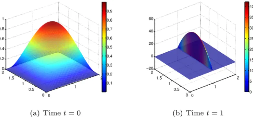
In case (iv), even if the initial condition is smooth, the magnetic advection with normally discontinuous collisional velocity yields the formation of a shock along the discontinuity (Figure11(b)) until complete blow up. An analogous behavior of the numerical magnetic potential obtained from the stabilized scheme can be reported in the case (ii), where instantaneous blow up of the solution along the discontinuity is observed. However, we expect a blow-up of the solution in these situations: the observed behavior of the numerical solution is not engendered by instabilities produced within the numerical scheme, but accurately reflects “physical reality”.
0 1 2 0 0.5 1 1.5 2 0 0.2 0.4 0.6 0.8 1 0.1 0.2 0.3 0.4 0.5 0.6 0.7 0.8 0.9 (a) Time t = 0 0 1 2 0 0.5 1 1.5 2 −20 0 20 40 60 0 5 10 15 20 25 30 35 40 (b) Time t = 1
Figure 11. First component of the numerical solution obtained from the stabilized scheme (cf as in (15)) with ⇤1h(Th) = Q1⇤1(Th) and Heun
method (⌧ = 0.1h), for collisional velocity and smooth initial condition as in (iv). 0 1 2 0 0.5 1 1.5 2 −1 −0.5 0 0.5 1 −0.8 −0.6 −0.4 −0.2 0 0.2 0.4 0.6 0.8 (a) Time t = 0.25 0 0.5 1 1.5 2 0 1 2 −1 −0.5 0 0.5 1 −0.6 −0.4 −0.2 0 0.2 0.4 0.6 (b) Time t = 0.75 0 1 2 0 0.5 1 1.5 2 −2 −1 0 1 2 x 10⁻⁹ −1 −0.5 0 0.5 1 x 10⁻⁹ (c) Time t = 2
Figure 12. First component of the magnetic potential obtained from the stabilized scheme (cf as in (15)) with ⇤1h(Th) =Q1⇤1(Th) and Heun
method (⌧ = 0.1h), for collisional velocity and smooth initial condition as in (iii).
6.4. Orszag-Tang benchmark. As last numerical experiment, we rely on a widely used two dimensional benchmark problem, the so-called Orszag-Tang vortex sys-tem [34], which describes the transition to supersonic turbulence in the MHD equa-tions. The development of shock waves and the complex interaction between various shocks with di↵erent speed which characterized the solution, makes the Orszag-Tang benchmark a challenging test for numerical methods.
Let us consider the two dimensional magnetic advection problem in ⌦ = [0, 2]2 with periodic boundary conditions at the boundary @⌦. The time interval is I = [0, 1] with uniform time step ⌧ = 5· 10 3. The initial condition is the smooth vector field u0(x, y) = (sin(2⇡x), sin(⇡y))>and the velocity field is piecewise constant with respect to the mesh. In particular, it is given at each time step as the outcome of a second order Finite Volume simulation of the full MHD system (from [33] and [21]). Note that even if the initial velocity is smooth, complex structures such as shocks and shock interactions develop in time. Concerning the discretization, the numerical scheme has been implemented on a tensor product mesh with 200⇥ 200 elements and H(curl, ⌦)-conforming lowest order rotated Raviart-Thomas elements ⇤1h(Th) =Q1⇤1(Th) have been used for the spatial discretization, while a second order two-stage Runge-Kutta timestepping is deployed in order to exploit the mild