HAL Id: hal-01062853
https://hal.archives-ouvertes.fr/hal-01062853
Preprint submitted on 12 Sep 2014
HAL is a multi-disciplinary open access
archive for the deposit and dissemination of
sci-entific research documents, whether they are
pub-lished or not. The documents may come from
teaching and research institutions in France or
abroad, or from public or private research centers.
L’archive ouverte pluridisciplinaire HAL, est
destinée au dépôt et à la diffusion de documents
scientifiques de niveau recherche, publiés ou non,
émanant des établissements d’enseignement et de
recherche français ou étrangers, des laboratoires
publics ou privés.
Schwarz methods for solving the time-harmonic Maxwell
equations
Mohamed El Bouajaji, Victorita Dolean, Martin J. Gander, Stéphane Lanteri,
Ronan Perrussel
To cite this version:
Mohamed El Bouajaji, Victorita Dolean, Martin J. Gander, Stéphane Lanteri, Ronan Perrussel.
Discontinuous Galerkin discretizations of optimized Schwarz methods for solving the time-harmonic
Maxwell equations. 2014. �hal-01062853�
SCHWARZ METHODS FOR SOLVING THE TIME-HARMONIC MAXWELL EQUATIONS
M. EL BOUAJAJI˚, V. DOLEAN:, M.J. GANDER; AND S. LANTERI˚, R. PERRUSSEL;
Abstract. We show in this paper how to properly discretize optimized Schwarz methods for the time-harmonic Maxwell equations using a discontinuous Galerkin (DG) method. Due to the multiple traces between elements in the DG formulation, it is not clear a priori how the more sophisticated transmission conditions in optimized Schwarz methods should be discretized, and the most natural approach does not lead at convergence of the Schwarz method to the mono-domain DG discretization, which implies that for such discretizations, the DG error estimates do not hold when the Schwarz method has converged. We present an alternative discretization of the transmission conditions in the framework of a DG weak formulation, and prove that for this discretization the multidomain and mono-domain solutions for the Maxwell’s equations are the same. We illustrate our results with several numerical experiments of propagation problems in homogeneous and heterogeneous media.
Key words. computational electromagnetism, time-harmonic Maxwell’s equations, Discontin-uous Galerkin method, optimized Schwarz methods, transmission conditions.
AMS subject classifications. 65M55, 65F10, 65N22
1. Introduction. Discontinuous Galerkin (DG) methods have received a lot of
attention over the last decade, since they combine the best of both finite element and finite volume methods. The approximation of each field is done locally at the level of each mesh element, by using a local basis of functions, and the discontinuity between neighboring elements is treated using a finite volume flux. A richer representation of the solution is given, at the price of increasing the total number of degrees of freedom as a result of the decoupling of the elements. The literature on these methods applied to different types of equations is rich and we will focus on contributions concerning Maxwell’s equations. A complete historical introduction with a large panel of references can be found in the milestone book on DG methods by Hesthaven and Warburton [24].
Theoretical results on DG methods applied to the time-harmonic Maxwell equa-tions have been obtained by several authors. Most of these use the second order formulation of the Maxwell equations. An alternative is to use the first order formu-lation as in [21, 22, 23], based on the theory of the Friedrichs systems. In a large part of the literature on time-harmonic problems, a mixed formulation is used (see [31, 26]), but DG methods on the non-mixed formulation like interior penalty techniques [25, 6] and local discontinuous Galerkin methods [6] have also been studied. A numerical convergence study of discontinuous Galerkin methods based on centered and upwind fluxes and nodal polynomial interpolation applied to the first-order time-harmonic Maxwell system in the two-dimensional case can be found in [12].
˚INRIA SOPHIA ANTIPOLIS-MÉDITERRANÉE, 06902 SOPHIA ANTIPOLIS CEDEX,
FRANCE.
:UNIV. DE NICE SOPHIA-ANTIPOLIS, LABORATOIRE J.-A. DIEUDONNÉ, NICE,
FRANCE. DOLEAN@UNICE.FR
;SECTION DE MATHÉMATIQUES, UNIVERSITÉ DE GENÈVE, CP 64, 1211 GENÈVE,
MARTIN.GANDER@MATH.UNIGE.CH
˚INRIA SOPHIA ANTIPOLIS-MÉDITERRANÉE, 06902 SOPHIA ANTIPOLIS CEDEX,
FRANCE.
;CNRS, UNIVERSITÉ DE TOULOUSE, LABORATOIRE PLASMA ET CONVERSION
D’ÉNERGIE, 31071 TOULOUSE CEDEX 7, FRANCE 1
Like for all other discretizations of the time-harmonic Maxwell equations, it is also difficult to solve linear systems obtained by DG discretizations with iterative methods. Due to the indefinite nature of the problems, classical iterative solvers fail as in the Helmholtz case [19]. Després defined in [9] a first provably convergent domain decomposition algorithm for the Helmholtz equation. This algorithm was extended to Maxwell’s equations in [10]. Even better transmission conditions were proposed in [7, 8, 20], based on optimized Schwarz theory, with an application to the second order Maxwell system in [1]. An entire hierarchy of optimized Schwarz methods for the first order Maxwell’s equations can be found in [15], with complete asymptotic results for the optimization. First DG discretizations of optimized Schwarz methods for time-harmonic Maxwell’s equations were proposed in [17] and [4]. Classical finite-element based non-overlapping and non-conforming domain decomposition methods for the computation of multiscale electromagnetic radiation and scattering problems can be found in [27, 30, 28, 32, 33, 29].
This paper is organized as follows: in Section 2 we present the time-harmonic Maxwell equations as a first order system, and introduce the notation for what fol-lows. In Section 3 we show the classical and optimized Schwarz algorithm at the continuous level for the first order Maxwell system. In Section 4, we introduce a weak formulation for the first order system, and then use a DG approximation to obtain discrete subdomain problems. We then show that while the DG discretization of the classical Schwarz method is very natural, optimized transmission conditions are more tricky to discretize, and we present a discretization for which we prove that the monodomain and multidomain formulations are equivalent. We then show in Section 5 several numerical experiments for both homogeneous and heterogeneous propagation problems to illustrate the performance of the optimized Schwarz methods as solvers for DG discretized Maxwell equations. Section 6 contains a brief conclusion.
2. The Time Harmonic Maxwell System. The time-harmonic Maxwell
equa-tions in a homogeneous medium are given by
iωεE´ curl H ` σE “ 0, iωµH` curl E “ 0, (2.1)
where the positive real parameter ω is the pulsation of the harmonic wave, σ is the electric conductivity, ε is the electric permittivity, µ magnetic permeability and the unknown complex-valued vector fields E and H are the electric and magnetic fields. In the homogeneous case to simplify the notation we can rewrite equation 2.1 as
i˜ωE´ curl H ` ˜σE “ 0, i˜ωH` curl E “ 0, (2.2)
where ˜ω :“ ω?εµ and ˜σ :“ σaµε. Collecting the variables into one big vector
W:“ pE, Hq, we can rewrite (2.2) as a first order system,
G0W` GxBxW` GyByW` GzBzW“ 0, (2.3) where G0:“ ˆ p˜σ ` i˜ωqI3ˆ3 03ˆ3 03ˆ3 i˜ωI3ˆ3 ˙ , and Gx:“ ˆ 03ˆ3 Nx NT x 03ˆ3 ˙ , Gy :“ ˆ 03ˆ3 Ny NT y 03ˆ3 ˙ , Gz:“ ˆ 03ˆ3 Nz NT z 03ˆ3 ˙ ,
with Nx:“ ¨ ˝ 0 0 0 0 0 1 0 ´1 0 ˛ ‚, Ny:“ ¨ ˝ 0 0 ´1 0 0 0 1 0 0 ˛ ‚, Nz:“ ¨ ˝ 0 1 0 ´1 0 0 0 0 0 ˛ ‚. For a general vector n“ pnx, ny, nzq, we can define the matrices
Gn:“ ˆ 03ˆ3 Nn NT n 03ˆ3, ˙ and Nn:“ ¨ ˝ 0 nz ´ny ´nz 0 nx ny ´nx 0 ˛ ‚.
The skew-symmetric matrix Nnallows us to define the cross product between a vector
Vand the vector n,
Vˆ n “ NnVand nˆ V “ NnTV. (2.4)
Moreover, if the vector n is normalized, we have also N3
n “ ´Nn. Using these
no-tations, the matrices Gl with l standing for tx, y, zu are in fact Gl “ Gel, where
el, l“ 1, 2, 3 are the canonical basis vectors.
We consider here a total field formulation, that is we are interested in the unknown
vector W“ Winc` Wscwhere Wincrepresents the incident field and Wscrepresents
the scattered field over an obstacle with boundary Γmor in an inhomogeneous medium.
Our goal is to solve the boundary-value problem whose strong form is given by
G0W` ÿ lPtx,y,zu GlBlW “ 0, in Ω, pMΓm´ GnqW “ 0 on Γm, pMΓa´ GnqpW ´ Wincq “ 0 on Γa. (2.5)
Here the matrices MΓm and MΓa are used for taking into account the boundary
conditions of the problem imposed on the metallic boundary Γm and the absorbing
boundary Γa, MΓm “ ˆ 03ˆ3 Nn ´NT n 03ˆ3 ˙ and MΓa“ |Gn|“ ˆ NnNnT 03ˆ3 03ˆ3 NnTNn ˙ .
We will use in what follows the matrices G`n and G´n which denote the positive and
negative parts of Gn according to its diagonalization. We note that |Gn|“ G`n´ G´n
and the definition of the G`n and G´n can be deduced from those of Gn and |Gn|,
G´n “ 1 2pGn´ |Gn|q and G ` n “ 1 2pGn` |Gn|q. (2.6)
3. Continuous classical and optimized Schwarz algorithms. We
decom-pose the computational domain Ω into two non-overlapping subdomains Ω1 and Ω2.
We denote by Σ the interface between Ω1and Ω2, by Wj the restriction of W to the
subdomain Ωj and by n the unit outward normal vector to Σ pointing from Ω1to Ω2.
Schwarz algorithms compute at each iteration step n“ 0, 1, 2, ... a new approximation
Wn`1
j from a given approximation Wjn, j“ 1, 2 by solving
G0Wn`11 ` ÿ lPtx,y,zu GlBlWn`11 “ 0, in Ω1, pG´ n` S1G`nqWn`11 “ pGn´` S1G`nqW2n, on Σ, G0Wn`12 ` ÿ lPtx,y,zu GlBlWn`12 “ 0, in Ω2, pG` n` S2G´nqWn`12 “ pGn`` S2G´nqW1n, on Σ, (3.1)
where S1 and S2 are differential operators. When S1 and S2 are equal to zero, the
algorithm is called classical Schwarz algorithm and it uses classical transmission con-ditions. It has been shown in [15] that these classical conditions have the meaning of imposing Dirichlet conditions on characteristic (incoming) variables in each subdo-main. Since G´n “ ˆ ´NnNnT Nn NT n ´NnTNn ˙ “ ˆI 3ˆ3 ´NT n ˙ ` ´NnNnT Nn ˘ , (3.2) G`n “ ˆ NnNnT Nn NT n NnTNn ˙ “ ˆ I3ˆ3 NT n ˙ ` NnNnT Nn ˘ , (3.3)
the classical transmission conditions are also equivalent to imposing impedance con-ditions, G´nW n`1 1 “ G´nW2n ðñ BnpE1n`1, Hn1`1q “ BnpEn2, Hn2q, G`nWn`12 “ G`nW1n ðñ B´npEn`12 , Hn`12 q “ B´npEn1, Hn1q, (3.4) where the impedance operator is given by
BnpE, Hq :“ NnNnTE´ NnH, (3.5)
and for subdomain Ω2we have used the fact that G`n “ ´G´´n. The classical Schwarz
algorithm has been thoroughly tested in [16] for the solution of the three-dimensional time-harmonic Maxwell equations discretized by low order DG methods.
In the second order formulation of Maxwell’s equation, the classical Schwarz method uses the impedance condition
˜
BnpEq “ p∇ ˆ E ˆ nq ˆ n ` i˜ωEˆ n, (3.6)
see [11]. This impedance condition is equivalent to using the condition ˜
BnpEq “ p∇ ˆ E ˆ nq ´ i˜ωnˆ pE ˆ nq, (3.7)
which is just a rotation by 90 degrees of (3.6), but is more adapted to variational formulations, see for example [5]. Condition (3.7) is equivalent to (3.5) if we replace
Hfrom Maxwell’s equation as a function of ∇ˆ E. The equivalence between the first
and second order formulation has been illustrated in [13] and [14]. As in (3.4), we also have the equivalences
pG´ n ` S1G`nqWn1`1“ pG´n` S1G`nqWn2 ðñ pBn` ˜S1B´nqpEn1`1, H n`1 1 q “ pBn` ˜S1B´nqpEn2, Hn2q, pG` n ` S2G´nqWn`12 “ pG`n` S2G´nqWn1 ðñ pB´n` ˜S2BnqpEn`12 , Hn`12 q “ pB´n` ˜S2BnqpEn1, Hn1q. (3.8)
Here ˜S1 and ˜S2 denote differential operators which are approximations of the
trans-parent operators and S1 and S2 are defined to guarantee the above equivalence. In
[18], an entire hierarchy of optimized algorithms, defined by the choice of ˜Sj, j“ 1, 2,
was obtained from the transparent operators. Using (3.2) and (3.3), the optimized transmission conditions (3.8) become
NnNnTE1n`1´ NnHn1`1` ˜S1pNnNnTEn1`1` NnHn1`1q
“ NnNnTEn2´ NnHn2` ˜S1pNnNnTEn2` NnHn2q,
NnNnTE2n`1` NnHn2`1` ˜S2pNnNnTEn2`1´ NnHn2`1q
“ NnNnTEn1` NnHn1` ˜S2pNnNnTEn1´ NnHn1q.
4. Discontinuous Galerkin approximation. We now present a weak formula-tion and a DG discretizaformula-tion of the Schwarz algorithms (3.1), and show how optimized transmission conditions are properly discretized in a DG framework.
4.1. Weak Formulation. We denote by Th a triangulation of the domain Ω,
by Γ0
, Γmand Γa the sets of purely internal, metallic and absorbing faces, by K an
element of Thand by F “ K X ˜Kthe face shared by two neighboring elements K and
˜
K. On each face F , we define the averagetWu and the tangential trace jump JWK of
Wby
tWu :“ 1
2pWK` WK˜q and JWK :“ GnKWK` GnK˜WK˜.
For two vector valued functions U and V inpL2
pDqq6 , we denote by pU, VqD:“ ż D U¨ V dx, if D is a domain of R3, and by xU, VyF “ ż F U¨ V ds,
if F is a two-dimensional face. For simplicity, we will skip the index for Th, i.e. we
write in what follows
p¨, ¨q :“ p¨, ¨qTh “
ÿ
KPTh
p¨, ¨qK.
On the boundaries we define
MF,K :“ $ ’ & ’ % ˆ ηFNnKNnTK NnK ´NT nK 03ˆ3 ˙ with ηF ‰ 0, if F belongs to Γm, |GnK| if F belongs to Γa.
We thus obtain a weak formulation of the problem,
pG0W, Vq ` ¨ ˝ ÿ lPtx,y,zu GlBlW, V ˛ ‚´ ÿ FPΓ0 xJWK, tVuyF` ÿ FPΓ0 B 1 2JWK, JVK F F ` ÿ FPΓmYΓa B 1 2pMF,K´ GnKqW, V F F “ ÿ FPΓa B 1 2pMF,K´ GnKqWinc, V F F . (4.1) 4.2. Discretization of the Subdomain Problems and Classical Schwarz
Algorithm. Let PppDq denote the space of polynomial functions of degree at most p
on a domain D. For any element KP Th, let DppKq ” pPppKqq6. The discontinuous
finite element spaces we use are then defined by Dp h“ VP pL 2 pΩqq6 | V|K P DppKq, @K P Th ( .
Approximate solutions W and test functions V for the discretized problem will be taken in the space Dph.
Let ΓΣbe the set of faces on the interface Σ, Γj0be the set of faces in the interior of
each subdomain Ωj, and Γjbbe the set of faces for each subdomain which lie on the real
boundaryBΩ. For any face F “ K X ˜K, note also that G2
nK “ G 2
nK˜ “ |GnK|“ |GnK˜|.
Then for each subdomain Ω1 and Ω2, the weak form can be written as
pG0W1, V1q ` ˜ ÿ l GlBlW1, V1 ¸ `ÿ Γ1 0 ˛ `ÿ Γ1 b ˛ ` ÿ FPΓΣ B 1 2p|GnK|´GnKq pW1´ W2q, V1 F F “ 0, pG0W2, V2q ` ˜ ÿ l GlBlW2, V2 ¸ `ÿ Γ2 0 ˛ `ÿ Γ2 b ˛ ` ÿ FPΓΣ B 1 2 ` |GnK˜|´GnK˜ ˘ pW2´ W1q, V2 F F “ 0, (4.2)
where, for simplicity, we have replaced some terms on the faces that do not play any
particular role in what follows by a ˛. For any face F “ K X ˜K on Σ, if n denotes
the normal on Σ directed from Ω1towards Ω2, and K and ˜Kare elements of Ω1and
Ω2, we have nK“ n “ ´nK˜.
The classical algorithm, which uses characteristic transmission conditions, corre-sponds in this DG formulation to a simple relaxation of the coupling flux terms in the
coupled formulation (4.2): starting from initial guesses W0
1 and W
0
2, it computes the
iterates Wn`1j from Wn
j, j“ 1, 2 by solving on Ω1 and Ω2the subproblems
` G0Wn`11 , V1 ˘ ` ˜ ÿ l GlBlWn`11 , V1 ¸ `ÿ Γ1 0 ˛ `ÿ Γ1 b ˛ ` ÿ FPΓΣ @ G´npW n`1 1 ´ Wn2q, V1 D F “ 0, ` G0Wn`12 , V2 ˘ ` ˜ ÿ l GlBlWn`12 , V2 ¸ `ÿ Γ2 0 ˛ `ÿ Γ2 b ˛ ` ÿ FPΓΣ @ G`npWn2`1´ Wn1q, V2 D F “ 0, (4.3)
where we used again (2.6) to simplify the notation. The relaxation in (4.3) is com-pletely natural in the context of a DG discretization: we simply replaced the
occur-rence of the flux G´nWn1`1 from outside the subdomain by the flux from the
neigh-boring subdomain G´nWn2 at the previous iteration, and vice versa, the occurrence of
G`nW2n`1by G`nWn1. This corresponds precisely to using the transmission conditions
in (3.1) with Sj “ 0, j “ 1, 2, namely
G´nWn1`1 “ G´nW2n
G`nWn`12 “ G`nW1n,
(4.4) and thus naturally guarantees at convergence of the associated classical Schwarz al-gorithm that the mono-domain DG solution is obtained. Such a simple replacement
is however not possible for optimized transmission conditions, Sj ‰ 0, and the
variables available in each subdomain, namely G´nW n`1 1 ` S1G`nW n`1 1 “ G´nW2n` S1G`nW2n, G`nWn`12 ` S2G´nWn`12 “ G`nW1n` S2G´nW1n, (4.5) leads to a DG solution obtained at convergence of the Schwarz algorithm which is different from the mono-domain DG solution, and thus for this different solution none of the DG error estimates hold. The solver should however never change the solution sought, and such a discretization is therefore to be avoided. We show in the next section how to properly discretize optimized transmission conditions in the framework of DG discretizations.
4.3. Discretization of Optimized Transmission Conditions. In order to
correctly introduce optimized transmission conditions (3.1) with non-zero Sj into the
DG discretization, we first write explicitly what transmission conditions the classical relaxation in (4.3) corresponds to. To do so, the subdomain problems solved in (4.3) are not allowed to depend on variables of the other subdomain anymore, since the coupling will be performed with the transmission conditions, and we thus need to introduce additional unknowns, namely Wn2,Ω1`1 on Ω1 and Wn1,Ω2`1 on Ω2, in order to
write the classical Schwarz iteration with local variables only, i.e. ` G0Wn`11 , V1 ˘ ` ˜ ÿ l GlBlWn`11 , V1 ¸ `ÿ Γ1 0 ˛ `ÿ Γ1 b ˛ ´ ÿ FPΓΣ A G´npW n`1 1 ´ W n`1 2,Ω1q, V1 E F “ 0, ` G0Wn`12 , V2 ˘ ` ˜ ÿ l GlBlWn`12 , V2 ¸ `ÿ Γ2 0 ˛ `ÿ Γ2 b ˛ ` ÿ FPΓΣ A G`npW2n`1´ W n`1 1,Ω2q, V2 E F “ 0. (4.6)
Comparing with the classical Schwarz algorithm (4.3), we see that in order to obtain the same algorithm, the transmission conditions for (4.6) need to be chosen as
G´nWn2,Ω1`1 “ G´nWn2, G`nW1,Ω2n`1 “ G`nW1n, (4.7)
which we have already seen when explicitly stating the relaxation as a replacement in (4.4). But one has to be careful when keeping these variables, since they represent the outside traces at the interface, not the inside traces of the elements! The transmission condition (4.7) implies that in the limit, when the algorithm converges, the so called coupling conditions
G´nW2,Ω1 “ G´nW2, G`nW1,Ω2 “ G`nW1, (4.8)
will be verified, where we dropped the iteration index to denote the limit quantities. These are the conditions which imply the same converged solution as the mono-domain DG solution. When using the Schwarz algorithm (4.6) with optimized transmission conditions (3.1), we therefore propose to use DG discretizations of the strong relations
G´nW n`1 2,Ω1` S1G`nW n`1 1 “ G´nWn2 ` S1G`nWn1,Ω2, G`nWn`11,Ω2` S2G ´ nWn`12 “ G`nW1n` S2G´nWn2,Ω1, (4.9)
which are substantially different from the transmission conditions (4.5), since they use
additional variables W2,Ω1 and W1,Ω2 which in principle belong to the traces at the
interface Σ of the neighboring subdomain, and are not available in the formulation (4.5). We will now prove that with the transmission conditions (4.9), at convergence of the associated Schwarz algorithm the same coupling conditions as (4.8) hold, and thus the optimized Schwarz method converges to the mono-domain solution of the DG discretization chosen. First, from (3.2) and (3.3), note that relation (4.8) is equivalent to # NnNnTE2,Ω1´ NnH2,Ω1 “ NnNnTE2´ NnH2, NnNnTE1,Ω2` NnH1,Ω2 “ NnN T nE1` NnH1. (4.10) We now introduce the auxiliary variables
Λ2,Ω1:“ NnNnTE2,Ω1´ NnH2,Ω1, Λ2:“ NnNnTE2´ NnH2,
Λ1,Ω2:“ NnNnTE1,Ω2` NnH1,Ω2, Λ1:“ NnNnTE1` NnH1. (4.11)
These variables represent traces belonging to a traced finite-element space Mhp“ ηP pL2pΣqq3 | η|F P pPppF qq3, pη ¨ nq|F “ 0, @F P Σ
(
. (4.12)
Note that Mhpconsists of vector-valued functions whose normal component is zero on
any face F P Σ. At convergence of the classical Schwarz algorithm, and hence for the
mono-domain DG solution, we see from (4.8) that these trace variables have to satisfy
Λ2,Ω1 “ Λ2, Λ1,Ω2 “ Λ1. (4.13)
From (4.9) and (4.13), we have to find for optimized transmission conditions a suitable DG discretization of the relations
Λ2,Ω1` ˜S1Λ1“ Λ2` ˜S1Λ1,Ω2, Λ1,Ω2` ˜S2Λ2“ Λ1` ˜S2Λ2,Ω1. (4.14)
In [18], it was shown that the optimized operators ˜Sj, j “ 1, 2, are second order
operators (see Table 4.1) where ˜ Qsj “ „ Bτ1τ1´ Bτ2τ2´ ˜σsj 2Bτ1τ2 2Bτ1τ2 Bτ2τ2´ Bτ1τ1´ ˜σsj ,
and the division by|k|2
indicates an integral operation. Note that the operator ˜Qsj
can be re-written as ˜ Qsj “ „ Bτ1τ1 Bτ1τ2 Bτ1τ2 Bτ2τ2 ` „ ´Bτ2τ2 Bτ1τ2 Bτ1τ2 ´Bτ1τ1 ´ ˜σsjId “ ∇loomoonτ∇τ¨ ST M ` ∇looooomooooonτˆ ∇τˆ ST E ´˜σsjId,
where Id denotes the identity operator, τj, j“ 1, 2 are two independent vectors in the
tangent plane to the interface, ∇τ denotes the gradient in the tangent plane to the
interface, ∇τ¨ is the divergence in the tangent plane and ∇τˆ is the two-dimensional
curl operator in the tangent plane. The operators ST M and ST E verify the remarkable
relation
Algorithm Fp ˜Sjq 1 0 2 s´i˜ω ps`i˜ωqp|k|2 `s˜σqFp ˜Qsq, sP C 3 1 |k|2 ´2˜ω2 `2i˜ω ˜σ`p2i˜ω`˜σqsFp ˜Qsq, sP C 4 psj`i˜ωsjqp|k|´i˜ω2 `sjσ˜qFp ˜Qsjq, sj P C 5 1 |k|2 ´2˜ω2 `2i˜ω ˜σ`p2i˜ω`˜σqsjFp ˜Qsjq, sjP C
Table 4.1: Symbols of the different operators
where ∆τ is the Laplace-Beltrami operator, and they act mainly on the transverse
electric and transverse magnetic part of the solution, see [13] and [14] for more details. To avoid an integral relation in the transmission condition, one has to multiply the entire transmission conditions by the operator symbol in the denominator, and then obtains second order differential transmission conditions. These second order dif-ferential transmission conditions are equivalent to the transmission conditions (4.14), and are of the form
˜
P1pΛ2,Ω1´ Λ2q “ ˜Qs1pΛ1,Ω2´ Λ1q,
˜
P2pΛ1,Ω2´ Λ1q “ ˜Qs2pΛ2,Ω1´ Λ2q,
(4.15) where for example for the Algorithms 2 and 4 indicated in Table 4.1 we have
˜ Pj:“
sj` i˜ω
sj´ i˜ωp´∆τ` ˜σsjqId,
sjP C, (4.16)
and for the Algorithms 3 and 5 we have ˜
Pj : “ p´∆τ´ 2˜ω2` 2i˜ω˜σ` 2i˜ωsj` ˜σsjqId
“ ST E´ ST M ` p´2˜ω2` 2i˜ω˜σ` 2i˜ωsj` ˜σsjqId, sj P C.
(4.17)
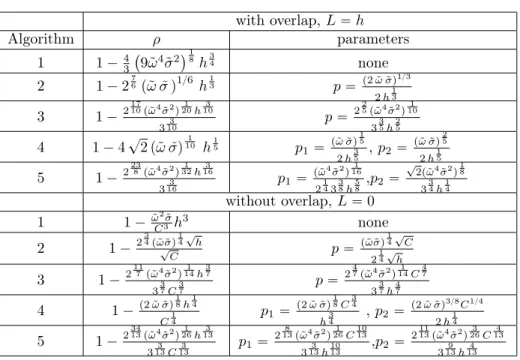
Here the parameters sj, j “ 1, 2 can be chosen to optimize the performance of the
method, see Table 4.2 for asymptotically optimized values.
Letpηjqj be a basis of Mhp. We define on the interface Σ the matrices
pMΣqi,j:“ ÿ FPΣ xηi, ηjyF, pKΣqi,j:“ ÿ FPΣ x∇τˆ ηi,∇τˆ ηjyF` x∇τ¨ ηi,∇τ¨ ηjyF ` ÿ ePBΣ ż e αh´1 ÿ kPt1,2u JJηi¨ τkKKJJηj¨ τkKK ´ ÿ ePBΣ ż ett∇ τ¨ ηiuu JJηj¨ ne,τKK´ JJηi¨ ne,τKK ∇τ¨ ηj (( ´ ÿ ePBΣ ż e tt∇τˆ ηiuu ¨ JJηjˆ ne,τKK´ JJηiˆ ne,τKK¨ ∇τˆ ηj (( ,
with overlap, L“ h Algorithm ρ parameters 1 1´4 3 ` 9˜ω4 ˜ σ2˘18 h34 none 2 1´ 276p˜ω ˜σq1{6 h 1 3 p“p2 ˜ω ˜σq 1{3 2 h 1 3 3 1´2 17 10p˜ω4σ˜2 q201h 3 10 3 3 10 p“ 2 2 5p˜ω4˜σ2 q101 3 3 5h 2 5 4 1´ 4?2p˜ω ˜σq101 h 1 5 p1“ p˜ω ˜σq 1 5 2 h 3 5 , p 2“ p˜ω ˜σq 2 5 2 h 1 5 5 1´2 23 8p˜ω4σ˜2q321h 3 16 3 3 16 p1“p˜ω 4 ˜ σ2q161 2 1 43 3 8h 5 8 ,p 2“ ? 2p˜ω4σ˜2q18 3 3 4h 1 4 without overlap, L“ 0 1 1´ω˜2 ˜ σ C3 h 3 none 2 1´2 3 4p˜ω ˜σq 1 4?h ? C p“ p˜ω ˜σq14?C 2 1 4?h 3 1´2 11 7 p˜ω4σ˜2q141h 3 7 3 3 7C 3 7 p“ 2 4 7p˜ω4σ˜2q141 C 4 7 3 3 7h 4 7 4 1´p2 ˜ω ˜σq 1 8h 1 4 C14 p1“p2 ˜ω ˜σq 1 8C 3 4 h34 , p 2“ p2 ˜ω ˜σq 3{8C1{4 2 h14 5 1´2 34 13p˜ω4σ˜2 q261h 3 13 3 3 13C 3 13 p 1“ 2 8 13p˜ω4σ˜2 q261C 10 13 3 3 13h 10 13 ,p 2“ 2 11 13p˜ω4σ˜2 q263C 4 13 3 9 13h 4 13
Table 4.2: Asymptotic convergence factor and optimal choice of the parameters in the transmission conditions. and pAΣqi,j :“ ÿ FPΣ x∇τˆ ηi,∇τˆ ηjyF ´ x∇τ¨ ηi,∇τ¨ ηjyF ` ÿ ePBΣ ż e αh´1 ÿ kPt1,2u JJηi¨ τkKKJJηj¨ τkKK ` ÿ ePBΣ ż ett∇ τ¨ ηiuu JJηj¨ ne,τKK´ JJηi¨ ne,τKK ∇τ¨ ηj (( , ´ ÿ ePBΣ ż ett∇ τˆ ηiuu ¨ JJηjˆ ne,τKK´ JJηiˆ ne,τKK¨ ∇τˆ ηj (( ,
where the positivity of the discretized operator is guaranteed for sufficiently large
α, BΣ denotes the set of interior edges of Σ, JJ¨KK and tt¨uu denote the jump and
the average at an edge e between values of the neighboring triangles, and ne,τ is
the outward normal on e in the tangent plane. Then matrix KΣ comes from the
discretization of´∆τ using a symmetric interior penalty approach [3, 2]. Note that
the´∆τ operator has to be taken in “vector” form, since it is applied topΛ2, ˜Ω1´ Λ2q,
which is a discretization of a vector quantity. MΣ is an interface mass matrix with
the same dimensions as the interface stiffness matrix KΣ, and AΣ represents the
discretization of the operator „
Bτ1τ1´ Bτ2τ2 2Bτ1τ2
2Bτ1τ2 Bτ2τ2´ Bτ1τ1
.
Then the DG discretization of (4.15) for the Algorithms 2 and 4 is s1` i˜ω s1´ i˜ωpK Σ` ˜σs1MΣqpΛ2,Ω1´ Λ2q “ pAΣ´ ˜σs1MΣqpΛ1,Ω2´ Λ1q, s2` i˜ω s2´ i˜ωpK Σ` ˜σs2MΣqpΛ1,Ω2´ Λ1q “ pAΣ´ ˜σs2MΣqpΛ2,Ω1´ Λ2q, (4.18)
and for the Algorithms 3 and 5 we get
pKΣ` α1MΣqpΛ2,Ω1´ Λ2q “ pAΣ´ ˜σs1MΣqpΛ1,Ω2´ Λ1q,
pKΣ` α2MΣqpΛ1,Ω2´ Λ1q “ pAΣ´ ˜σs2MΣqpΛ2,Ω1´ Λ2q,
(4.19) where αj “ 2i˜ωpi˜ω` ˜σq ` 2i˜ωsj` ˜σsj. In the following theorem we will only treat the
case of Algorithms 3 and 5, similar techniques can be applied for Algorithms 2 and 4.
Theorem 4.1 (DG discretization of Algorithms 3 and 5). If s1 and s2 are
such that sj “ pjp1 ` iq with pj a strictly positive real number for j “ 1, 2, and
˜
σpp1´ p2q “ 0, then the relations (4.13) and (4.19) are equivalent.
Proof. We first see that ℑαj“ 2˜ω˜σ` 2˜ωpj` ˜σpją 0. Let us denote by
U1“ Λ1,Ω2´ Λ1, U2“ Λ2,Ω1´ Λ2.
Multiplying the first relation in (4.19) on the left by ¯UT
2 and the second by ¯UT1 and
summing them, we get ¯
UT2pKΣ`α1MΣqU2` ¯UT1pKΣ`α2MΣqU1“ ¯UT2pAΣ´˜σs1MΣqU1` ¯UT1pAΣ´˜σs2MΣqU2.
(4.20)
Since KΣis symmetric and non-negative, MΣis symmetric and positive definite, and
AΣ is symmetric, all the quantities ¯UTjMΣUj, ¯UTjKΣUj and ¯UT1AΣU2` ¯UT2AΣU1
are real. In this case, by taking the imaginary part of the previous relation we get ℑα1U¯T2MΣU2` ℑα2U¯T1MΣU1` ˜σℑps1U¯T2MΣU1` s2U¯T1MΣU2q “ 0. (4.21)
In order to simplify the notation, using that MΣ is symmetric positive definite, we
introduce the norm}U}2
MΣ :“ ¯UTMΣU, which is induced by the hermitian product
pU1, U2qMΣ“ ¯UT2MΣU1. Since by definitionpU2, U1qMΣ “ ĞpU1, U2qMΣ, we see that
ℑp ¯UT
2MΣU1q “ 2i1ppU1, U2qMΣ´ pU2, U1qMΣq “ ´ℑp ¯UT1MΣU2q,
ℜp ¯UT
2MΣU1q “ 12ppU1, U2qMΣ` pU2, U1qMΣq “ ℜp ¯UT1MΣU2q,
ℑps1U¯T2MΣU1q “ p1pℜpU1, U2qMΣ` ℑpU1, U2qMΣq,
ℑps2U¯T1MΣU2q “ p2pℜpU2, U1qMΣ` ℑpU2, U1qMΣq “ p2pℜpU1, U2qMΣ´ ℑpU1, U2qMΣq.
Also let p1“ p ` δ and p2“ p ´ δ and suppose δ ě 0. Then (4.21) becomes
2˜ωp˜σ ` p1q}U2}2MΣ` 2˜ωp˜σ ` p2q}U1}2MΣ` ˜σpp ` δq}U2}2MΣ` ˜σpp ´ δq}U1}2MΣ
`˜σpp ` δqpℜpU1, U2qMΣ` ℑpU1, U2qMΣq `˜σpp ´ δqpℜpU1, U2qMΣ´ ℑpU1, U2qMΣq “ 0 ô 2˜ωp˜σ ` p1q}U2} 2 MΣ` 2˜ωp˜σ ` p2q}U1} 2 MΣ `˜σpp}U2} 2 MΣ` }U1} 2 MΣ` 2ℜpU1, U2qMΣq `˜σδp}U2}2MΣ´ }U1} 2 MΣ` 2ℑpU1, U2qMΣq “ 0,
ô 2˜ωp˜σ ` p1q}U2}2MΣ` 2˜ωp˜σ ` p2q}U1}2MΣ` ˜σp}U1` U2}2MΣ
`˜σδp}U2} 2 MΣ´ }U1} 2 MΣ` 2ℑpU1, U2qMΣq “ 0. (4.22)
We thus see that if ˜σ “ 0 or δ “ 0, which means p1 “ p2 (Algorithm 3 from Table
4.2), then the last form of (4.22) leads to the conclusion that Uj “ 0, since all the
4.4. Two-dimensional case. Like in the three-dimensional case, we can rewrite (4.9) and (4.8) by introducing the auxiliary variables (see [4] for more details)
Λ2,Ω1 :“ E2,Ω1´ NnH2,Ω1, Λ2:“ E2´ NnH2,
Λ1,Ω2 :“ E1,Ω2` NnH1,Ω2, Λ1:“ E1` NnH1,
(4.23)
belonging to the trace space Mhp “ ηP L2
pΣq | η|F P PppF q, @F P Σ
(
. Then (4.8) becomes
Λ2,Ω1 “ Λ2 and Λ1,Ω2 “ Λ1. (4.24)
From (4.9) and (4.23), we see that we have to find for optimized transmission condi-tions a suitable DG discretization of the relacondi-tions
Λ2,Ω1` ˜S1Λ1“ Λ2` ˜S1Λ1,Ω2 and Λ1,Ω2` ˜S2Λ2“ Λ1` ˜S2Λ2,Ω1. (4.25)
If we focus on the second order transmission conditions, (4.25) becomes p´B2 τ` i˜ω˜σ´ 2˜ω 2 ` 2i˜ωs1qpΛ2,Ω1´ Λ2q ` p´Bτ2` i˜ω˜σqpΛ1,Ω2´ Λ1q “ 0, p´B2 τ` i˜ω˜σ´ 2˜ω 2 ` 2i˜ωs2qpΛ1,Ω2´ Λ1q ` p´Bτ2` i˜ω˜σqpΛ2,Ω1´ Λ2q “ 0. (4.26)
Letpηjqj be a basis of Mhp. We define the matrices
pMΣqi,j :“ ÿ FPΣ xηi, ηjyF, pKΣqi,j :“ ÿ FPΣ xBτηi,BτηjyF` ÿ nPΣ0 αnh´1rrrrηissssnrrrrηjssssn ´ ÿ nPΣ0 ttBτηiuunrrrrηjssssn´ rrrrηissssnttBτηjuun,
where positiveness is guaranteed for sufficiently large αn, Σ0denotes the set of interior
nodes of Σ,rrrr¨ssssnandtt¨uundenotes the jump and the average at a node n between
values of the neighboring segments. The matrix KΣcomes from the discretization of
´B2
τ using a symmetric interior penalty approach [2].
The DG discretization of (4.26) is then
pKΣ` α1MΣqpΛ2,Ω1´ Λ2q “ p´KΣ´ i˜ω˜σMΣqpΛ1,Ω2´ Λ1q,
pKΣ` α2MΣqpΛ1,Ω2´ Λ1q “ p´KΣ´ i˜ω˜σMΣqpΛ2,Ω1´ Λ2q,
(4.27) with αj“ ´2˜ω2` ip˜ω˜σ` 2˜ωpjq. As in the three-dimensional case, KΣ is symmetric
and non-negative definite, and MΣis symmetric and positive definite. A similar result
to Theorem 4.1 can be obtained also in 2d:
Theorem 4.2 (DG discretization for the second order conditions in 2d). If s1
ands2are such thatsj “ pjp1 ` iq with pj a strictly positive real number forj “ 1, 2,
then the relations (4.24) and (4.27) are equivalent.
Proof. We first note that ℑαj“ ˜ω˜σ` 2˜ωpj ą 0. Setting
U1“ Λ1,Ω2´ Λ1, U2“ Λ2,Ω1´ Λ2,
and multiplying the first relation in (4.27) on the left by ¯UT
2, the second by ¯UT1, and
adding them, we obtain by taking the imaginary part
p˜ω˜σ` 2˜ωpjqp ¯UT1MΣU1` ¯UT2MΣU2q “ ´˜ω˜σp ¯UT2MΣU1` ¯UT1MΣU2q
By re-arranging the terms and using the norm notation we get 2˜ωpjp}U1}2MΣ` }U2}MΣ2 q ` ˜ω˜σ}U1` U2}2MΣ “ 0.
From this last equation, we see that Uj “ 0, since all the terms are positive, which
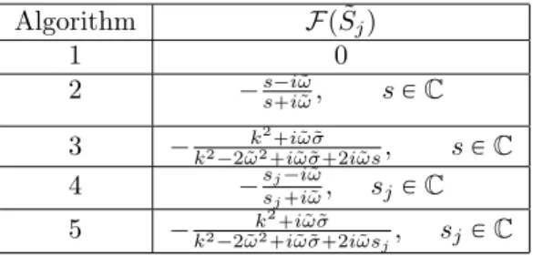
Algorithm Fp ˜Sjq 1 0 2 ´s´i˜ω s`i˜ω, sP C 3 ´ k2 `i˜ω ˜σ k2 ´2˜ω2 `i˜ω ˜σ`2i˜ωs, sP C 4 ´sj´i˜sj`i˜ωω, sj P C 5 ´ k2 `i˜ω ˜σ k2 ´2˜ω2 `i˜ω ˜σ`2i˜ωsj, sj P C
Table 5.1: Symbols of the different operators
without overlap Algorithm ρ parameters 1 1´ω˜2 ˜ σ C3 h 3 none 2 1´2 3 4p˜ω ˜σq 1 4?h ? C p“ p˜ω ˜σq14?C 2 1 4?h 3 1´2 11 7p˜ω4σ˜2 q141 h 3 7 3 3 7C 3 7 p“2 4 7p˜ω4σ˜2 q141 C 4 7 3 3 7h 4 7 4 1´p2 ˜ω ˜σq 1 8h 1 4 C14 p1“ p2 ˜ω ˜σq 1 8C 3 4 h34 , p2“ p2 ˜ω ˜σq3{8C1{4 2 h14 5 1´2 34 13p˜ω4˜σ2q261h 3 13 3 3 13C 3 13 p 1“ 2 8 13p˜ω4σ˜2q261C 10 13 3 3 13h 10 13 ,p 2“ 2 11 13p˜ω4σ˜2q263C 4 13 3 9 13h 4 13
Table 5.2: Asymptotic convergence factor and optimal choice of the parameters in the transmission conditions.
5. Numerical results. We illustrate the performance of the optimized Schwarz
algorithms discretized using a DG method in two dimensions. We consider the TM
formulation of Maxwell’s equations, i.e. E“ p0, 0, EzqT and H“ pHx, Hy, 0qT. We
can then rewrite the algorithm (3.1) by using that now W“ pEz, Hx, HyqT, and the
corresponding G-matrices are
G0“ ˆ ˜ σ` i˜ω 01ˆ2 02ˆ1 i˜ωI2ˆ2 ˙ , Gx“ ˆ 0 Nex NT ex 0 ˙ , Gy“ ˆ 0 Ney NT ey 0 ˙ , where Nn“ pny,´nxqT. We give in Table 5.1 the corresponding Fourier symbols of ˜Sj
in the two-dimensional case, which were derived from the 3d results given in [18]. The parameters s“ pp1 ` iq, s1“ p1p1 ` iq and s2“ p2p1 ` iq are solutions of specific
min-max problems solved in [18], and their asymptotic behavior in the homogeneous non-overlapping case is shown in Table 5.2, together with the corresponding convergence
factors and the constant C is defined such that kmax “ Ch is the highest numerical
frequency that can be represented by the discretization method on a mesh with mesh size h.
The Fourier symbols of the operators in Algorithms 1, 2 and 4 are constants, therefore their expression is the same in physical space. In this case (3.8) can be written in the 2d situation considered here as
#
E1n`1´ NnHn1`1` ˜S1pE1n`1` NnH1n`1q “ E2n´ NnHn2 ` ˜S1pE2n` NnHn2q,
E2n`1` NnHn`12 ` ˜S2pE2n`1´ NnHn`12 q “ E1n` NnHn1 ` ˜S2pE1n´ NnHn1q.
This is not the case for algorithms 3 and 5, where second order transmission conditions
result, because k2 appears in the corresponding Fourier symbols. As in the 3d case,
we need to rewrite the transmission conditions: the ˜Sj are operators whose Fourier
symbol can be written as Fp ˜Sjq “
qjpkq
rjpkq
with qjpkq “ ´pk2` i˜ω˜σq, rjpkq “ k2´ 2˜ω2` i˜ω˜σ` 2i˜ωsj.
We see that for the numerator and denominator separately, F´1pqjq and F´1prjq are
partial differential operators in the tangential direction, F´1qj “ Bτ τ´ i˜ω˜σ,F´1rj “ ´Bτ τ ´ 2˜ω
2
` i˜ω˜σ` 2i˜ωsj.
In this case, we multiply the transmission conditions on both sides by the denominator, and the interface iteration (5.1) can then be re-written as
$ ’ ’ & ’ ’ % F´1r 1pE1n`1´ NnHn`11 q ` F´1q1pE1n`1` NnHn`11 q “ F´1r1pEn 2 ´ NnHn2q ` F´1q1pE2n` NnHn2q, F´1r2pEn`1 2 ` NnHn2`1q ` F´1q2pE2n`1´ NnHn2`1q “ F´1r2pEn 1 ` NnHn1q ` F´1q2pE1n´ NnHn1q, (5.2) similarly to the general 3d case we explained in (4.15).
5.1. Plane wave in a homogeneous conductive medium. We consider first
the propagation of a plane wave in a homogeneous conductive medium. The
compu-tational domain is Ω“ p0, 1q2
, and ˜σ“ 0.5. We use DG discretizations with several
polynomial orders, denoted by DG-Pk, with k“ 1, 2, 3, 4, and impose on BΩ “ Γa an
incident wave Winc“ ¨ ˚ ˚ ˚ ˝ ky ˜ ω ´kx ˜ ω 1 ˛ ‹ ‹ ‹ ‚e ´ik¨x, and k“ ˆ kx ky ˙ “ ¨ ˝˜ω c 1´ iσ˜ ˜ ω 0 ˛ ‚. (5.3)
The domain Ω is decomposed into two subdomains Ω1 “ p0, 0.5q ˆ p0, 1q and Ω2 “
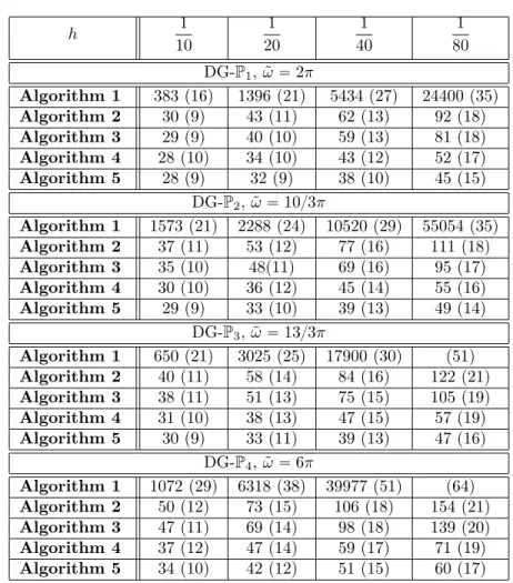
p0.5, 1q ˆ p0, 1q. The goal of this first test problem is to retrieve numerically the asymptotic behavior of the convergence factors of the optimized Schwarz methods when discretized using DG, and to compare with the theoretical convergence factors shown in Table 5.2. The iteration numbers to reduce the relative residual by six orders of magnitude are given in Table 5.3, where also the iteration numbers are given in parentheses for the use of the Schwarz methods as preconditioners for a Krylov method, which is BiCGStab in our case. We clearly see that there is a hierarchy of faster and faster algorithms, and their asymptotic behavior corresponds well to the analysis, as one can see from Figure 5.1.
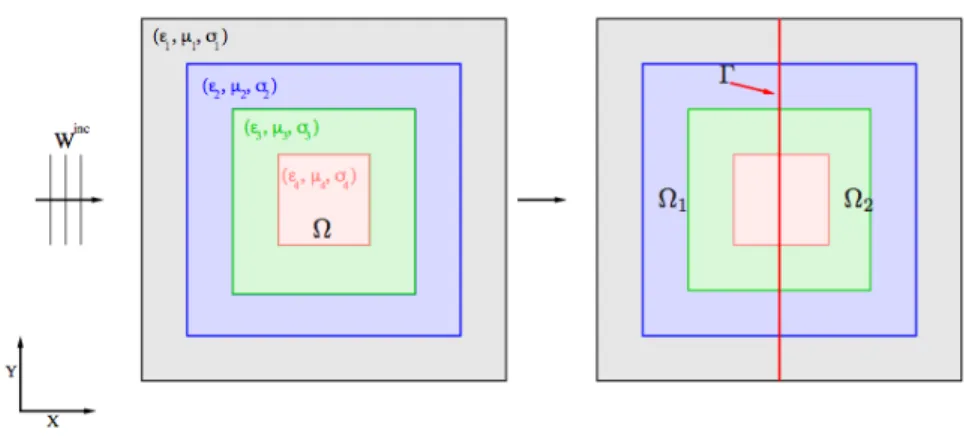
5.2. Plane wave in a multi-layer heterogeneous medium. We study now
the performance of the optimized Schwarz algorithms in the case of a heteroge-neous propagation medium. The model problem we consider is the propagation of a plane wave in a multi-layer conductive medium, as shown in Figure 5.2 on the
left. We decompose the computational domain Ω “ p´1, 1q2 into two subdomains
Ω1“ p0, 0.5q ˆ p0, 1q and Ω2“ p0.5, 1q ˆ p0, 1q, as shown in Figure 5.2 on the right.
10ï1 102 h Iterations Alg. 2 O(hï1/2) Alg. 3 O(hï3/7) Alg. 4 O(hï1/4) Alg. 5 O(hï3/13) 10ï1 102 h Iterations Alg. 2 O(hï1/2) Alg. 3 O(hï3/7) Alg. 4 O(hï1/4) Alg. 5 O(hï3/13) 10ï1 102 h Iterations Alg. 2 O(hï1/2) Alg. 3 O(hï3/7) Alg. 4 O(hï1/4) Alg. 5 O(hï3/13) 10ï1 102 h Iterations Alg. 2 O(hï1/2) Alg. 3 O(hï3/7) Alg. 4 O(hï1/4) Alg. 5 O(hï3/13)
Fig. 5.1: Asymptotic behavior of the iteration numbers from Table 5.3 as a function
of the mesh size h for the DG-P1, DG-P2, DG-P3,and DG-P4 discretizations.
Fig. 5.2: Domain configuration for the model problem of scattering of a plane wave in a multi-layer domain.
h 1 10 1 20 1 40 1 80 DG-P1, ˜ω“ 2π Algorithm 1 383 (16) 1396 (21) 5434 (27) 24400 (35) Algorithm 2 30 (9) 43 (11) 62 (13) 92 (18) Algorithm 3 29 (9) 40 (10) 59 (13) 81 (18) Algorithm 4 28 (10) 34 (10) 43 (12) 52 (17) Algorithm 5 28 (9) 32 (9) 38 (10) 45 (15) DG-P2, ˜ω“ 10{3π Algorithm 1 1573 (21) 2288 (24) 10520 (29) 55054 (35) Algorithm 2 37 (11) 53 (12) 77 (16) 111 (18) Algorithm 3 35 (10) 48(11) 69 (16) 95 (17) Algorithm 4 30 (10) 36 (12) 45 (14) 55 (16) Algorithm 5 29 (9) 33 (10) 39 (13) 49 (14) DG-P3, ˜ω“ 13{3π Algorithm 1 650 (21) 3025 (25) 17900 (30) (51) Algorithm 2 40 (11) 58 (14) 84 (16) 122 (21) Algorithm 3 38 (11) 51 (13) 75 (15) 105 (19) Algorithm 4 31 (10) 38 (13) 47 (15) 57 (19) Algorithm 5 30 (9) 33 (11) 39 (13) 47 (16) DG-P4, ˜ω“ 6π Algorithm 1 1072 (29) 6318 (38) 39977 (51) (64) Algorithm 2 50 (12) 73 (15) 106 (18) 154 (21) Algorithm 3 47 (11) 69 (14) 98 (18) 139 (20) Algorithm 4 37 (12) 47 (14) 59 (17) 71 (19) Algorithm 5 34 (10) 42 (12) 51 (15) 60 (17)
Table 5.3: Wave propagation in a homogeneous medium. Iteration count as a func-tion of h when the optimized Schwarz methods are used as iterative solvers, and in parentheses when used as preconditioners.
Layer i εi σ˜i µi DG-Pi
1 1.0 0.0 1 1
2 2.25 0.1 1 2
3 3.5 0.2 1 3
4 5.3 0.5 1 4
Table 5.4: Characteristic parameters of the medium for the model problem of scat-tering of a plane wave in a multi-layer domain.
We test here the method DG-P1,2,3,4 where the interpolation degree is fixed for
each element of the mesh according to the local wavelength, see the last column in Table 5.4. We show again the iteration numbers we obtain from the various optimized Schwarz algorithms to reduce the relative residual by 6 orders of magnitude in Table 5.5, and the corresponding iteration numbers when the Schwarz methods are used as
h 1 20 1 40 1 80 1 160 Algorithm 1 727 (31) 2974 (41) 11973 (52) (70) Algorithm 2 108 (21) 153(25) 220 (30) 315 (33) Algorithm 3 101 (20) 138 (23) 197 (27) 267 (30) Algorithm 4 87 (18) 103 (22) 128 (25) 157 (28) Algorithm 5 84 (16) 96 (20) 113 (22) 140 (25)
Table 5.5: Scattering of a plane wave in a multi-layer domain. Iteration count as a function of h when the optimized Schwarz methods are used as iterative solvers, and in parentheses when used as preconditioners.
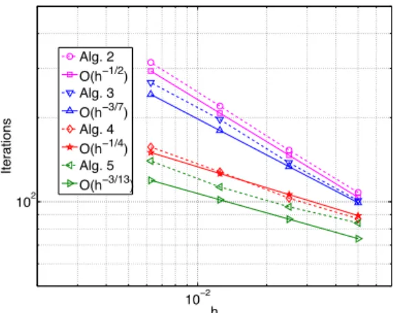
10ï2 102 h Iterations Alg. 2 O(hï1/2) Alg. 3 O(hï3/7) Alg. 4 O(hï1/4) Alg. 5 O(hï3/13)
Fig. 5.3: Asymptotic behavior of the iteration numbers from Table 5.5 as a function of the mesh size h.
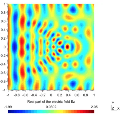
preconditioners in parentheses. In Figure 5.3, we plot these iteration numbers as a function of the mesh size, and also the corresponding theoretical asymptotic iteration number counts, which shows that even in such a layered medium, where our analysis is not valid any more, the Schwarz algorithms still behave asymptotically as the constant medium theory indicates. We finally show in 5.4 the real part of the electric field for this scattering problem.
5.3. Scattering of a plane wave by a conductive dielectric cylinder. The final model problem we consider is the scattering of a plane wave by a dielectric
conductive cylinder with radius r0“ 0.6 m. The computational domain is obtained by
artificially restricting the domain to a cylinder with radius r“ 1.6 m, and using the
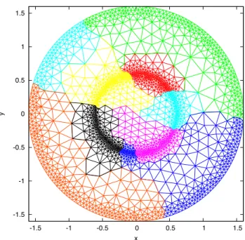
Silver-Müller condition on the artificial boundary. We use a non-uniform triangular mesh which consists of 2078 vertices and 3958 triangles, see Figure 5.5. The relative
permittivity of the inner cylinder is set to εr “ 2.25 and its electric conductivity to
˜
σ “ 0.01, while vacuum is assumed for the rest of the domain. The frequency we
consider is F=300 MHz. Numerical simulations are performed using decompositions into 4 and 16 subdomains, for an example see Figure 5.5. We show the iteration numbers for the various optimized Schwarz methods to reduce the relative residual by
Fig. 5.4: Real part of the electric field for the scattering of a plane wave in a multi-layer domain.
6 orders of magnitude in Table 5.6. Here, DG-P1,2,3,4 stands for a non-uniform order
DG discretization, i.e. the interpolation order is defined on an elementwise basis: small elements use low order shape functions, and large elements use high order ones. We note that the optimized algorithms improve substantially the convergence of the classical Schwarz algorithm (Algorithm 1 in the table) and also that the gain between both the optimized and the classical algorithms seems to slightly increase with the interpolation order. Finally, we also observe, as could be expected, a dependence of the iteration count on the number of subdomains, since we are not using any coarse grid correction in these experiments.
6. Conclusions. We have shown in this paper how optimized Schwarz methods
can be properly discretized in the framework of DG-methods, such that at conver-gence, the result of the underlying DG mono-domain solution is recovered. The key idea is to introduce additional trace variables on each subdomain interface represent-ing the DG-traces of the neighborrepresent-ing subdomain interface traces, and then to use both traces appropriately to discretize the optimized transmission conditions. We have tested the performance of the DG-discretized Schwarz methods on many numer-ical scattering experiments, both for homogeneous and heterogeneous media, and in various physical configurations and for various decompositions. Our numerical results indicate that the asymptotic performance of these algorithms obtained at a theoretical level for homogeneous media and constant coefficients well predicts the performance
-1.5 -1 -0.5 0 0.5 1 1.5 -1.5 -1 -0.5 0 0.5 1 1.5 y x
Fig. 5.5: Mesh and subdomain decomposition for the scattering problem of a plane wave by a dielectric conductive cylinder.
Method Algo 1 Algo 2 Algo 3 Algo 4 Algo 5 #of domains
DG-P1 76 33 32 29 28 4 - 104 50 47 45 42 16 DG-P2 99 40 38 36 33 4 - 145 62 57 53 50 16 DG-P3 124 50 46 44 40 4 - 168 66 62 58 55 16 DG-P4 134 52 48 42 39 4 - 203 81 75 70 76 16 DG-P1,2,3,4 78 34 31 29 28 4 - 105 51 48 46 44 16
Table 5.6: Scattering of a plane wave by a dielectric conductive cylinder. Iteration count vs. mesh size.
of the algorithms when discretized using DG-discretizations, both in homogeneous and heterogeneous media, and for very general decompositions.
REFERENCES
[1] A. Alonso-Rodriguez and L. Gerardo-Giorda. New nonoverlapping domain decomposition meth-ods for the harmonic Maxwell system. SIAM J. Sci. Comput., 28(1):102–122, 2006. [2] D. Arnold, F. Brezzi, B. Cockburn, and L. Marini. Unified analysis of Discontinuous Galerkin
[3] D. N. Arnold. An interior penalty finite element method with discontinuous elements. SIAM Journal on Numerical Analysis, 19(4):pp. 742–760, 1982.
[4] M. E. Bouajaji, V. Dolean, M. J. Gander, S. Lanteri, and R. Perrussel. DG discretization of optimized Schwarz methods for Maxwell’s equations. In J. Erhel, M. J. Gander, L. Halpern, T. Sassi, and O. Widlund, editors, Proceedings of the 21st international domain decompo-sition conference. Springer LNCSE, 2013.
[5] A. Buffa, M. Costabel, and D. Sheen. On traces for H(curl, Ω) in Lipschitz domains. Journal of Mathematical Analysis and Applications, 276(2):845–867, 2002.
[6] A. Buffa and I. Perugia. Discontinuous Galerkin approximation of the Maxwell eigenproblem. SIAM J. Numer. Anal., 44(5):2198–2226, 2006.
[7] P. Chevalier and F. Nataf. An OO2 (Optimized Order 2) method for the Helmholtz and Maxwell equations. In 10th International Conference on Domain Decomposition Methods in Science and in Engineering, pages 400–407, Boulder, Colorado, USA, 1997. AMS. [8] P. Collino, G. Delbue, P. Joly, and A. Piacentini. A new interface condition in the
non-overlapping domain decomposition for the Maxwell equations. Comput. Methods Appl. Mech. Engrg., 148:195–207, 1997.
[9] B. Després. Décomposition de domaine et problème de Helmholtz. C.R. Acad. Sci. Paris, 1(6):313–316, 1990.
[10] B. Després, P. Joly, and J. Roberts. A domain decomposition method for the harmonic Maxwell equations. In Iterative methods in linear algebra, pages 475–484, Amsterdam, 1992. North-Holland.
[11] B. Després, P. Joly, and J. E. Roberts. A domain decomposition method for the harmonic Maxwell equations. In Iterative methods in linear algebra (Brussels, 1991), pages 475–484, Amsterdam, 1992. North-Holland.
[12] V. Dolean, H. Fol, S. Lanteri, and R. Perrussel. Solution of the time-harmonic Maxwell equa-tions using discontinuous Galerkin methods. J. Comput. Appl. Math., 218(2):435–445, 2008.
[13] V. Dolean, M. J. Gander, S. Lanteri, J.-F. Lee, and Z. Peng. Optimized Schwarz methods for curl-curl time-harmonic Maxwell’s equations. In J. Erhel, M. J. Gander, L. Halpern, T. Sassi, and O. Widlund, editors, Proceedings of the 21st international domain decompo-sition conference. Springer LNCSE, 2013.
[14] V. Dolean, M. J. Gander, J.-F. Lee, and Z. Peng. Effective Transmission Conditions for Domain Decomposition Methods applied to the Time-Harmonic Curl-Curl Maxwell’s equations. submitted, 2014.
[15] V. Dolean, L. Gerardo-Giorda, and M. J. Gander. Optimized Schwarz methods for Maxwell equations. SIAM J. Scient. Comp., 31(3):2193–2213, 2009.
[16] V. Dolean, S. Lanteri, and R. Perrussel. A domain decomposition method for solving the three-dimensional time-harmonic Maxwell equations discretized by discontinuous Galerkin methods. J. Comput. Phys., 227(3):2044–2072, 2008.
[17] V. Dolean, S. Lanteri, and R. Perrussel. Optimized Schwarz algorithms for solving time-harmonic Maxwell’s equations discretized by a discontinuous Galerkin method. IEEE. Trans. Magn., 44(6):954–957, 2008.
[18] M. El Bouajaji, V. Dolean, M. J. Gander, and S. Lanteri. Optimized Schwarz methods for the time-harmonic Maxwell equations with dampimg. SIAM J. Scient. Comp., 34(4):2048– 2071, 2012.
[19] O. Ernst and M. Gander. Why it is difficult to solve Helmholtz problems with classical iterative methods. In I. Graham, T. Hou, O. Lakkis, and R. Scheichl, editors, Numerical Analysis of Multiscale Problems, pages 325–363. Springer Verlag, 2012.
[20] M. J. Gander, F. Magoulès, and F. Nataf. Optimized Schwarz methods without overlap for the Helmholtz equation. SIAM J. Sci. Comput., 24(1):38–60, 2002.
[21] P. Helluy. Résolution numérique des équations de Maxwell harmoniques par une méthode d’éléments finis discontinus. PhD thesis, Ecole Nationale Supérieure de l’Aéronautique, 1994.
[22] P. Helluy and S. Dayma. Convergence d’une approximation discontinue des systèmes du premier ordre. C. R. Acad. Sci. Paris, 319:1331–1335, 1994.
[23] P. Helluy, P. Mazet, and P. Klotz. Sur une approximation en domaine non borné des équa-tions de Maxwell instationnaires: comportement asymptotique. La Recherche Aérospatiale, 5:365–377, 1994.
[24] J. Hesthaven and T. Warburton. Nodal Discontinuous Galerkin methods: algorithms, analysis and applications. Springer, 2008.
[25] P. Houston, I. Perugia, A. Schneebeli, and D. Schötzau. Interior penalty method for the indefinite time-harmonic Maxwell equations. Numer. Math., 100(3):485–518, 2005.
[26] P. Houston, I. Perugia, A. Schneebeli, and D. Schötzau. Mixed discontinuous Galerkin approxi-mation of the Maxwell operator: the indefinite case. ESAIM: Math. Model. Numer. Anal., 39(4):727–753, 2005.
[27] S.-C. Lee, M. Vouvakis, and J.-F. Lee. A non-overlapping domain decomposition method with non-matching grids for modeling large finite antenna arrays. J. Comput. Phys., 203(1):1– 21, 2005.
[28] Z. Peng and J.-F. Lee. Non-conformal domain decomposition method with second-order trans-mission conditions for time-harmonic electromagnetics. J. Comput. Phys., 229(16):5615– 5629, 2010.
[29] Z. Peng and J.-F. Lee. A scalable nonoverlapping and nonconformal domain decomposition method for solving time-harmonic maxwell equations in rˆ3. SIAM Journal on Scientific Computing, 34(3):A1266–A1295, 2012.
[30] Z. Peng, V. Rawat, and J.-F. Lee. One way domain decomposition method with second order transmission conditions for solving electromagnetic wave problems. J. Comput. Phys., 229(4):1181–1197, 2010.
[31] I. Perugia, D. Schötzau, and P. Monk. Stabilized interior penalty methods for the time-harmonic Maxwell equations. Comput. Methods Appl. Mech. Engrg., 191(41-42):4675–4697, 2002. [32] V. Rawat. Finite Element Domain Decomposition with Second Order Transmission Conditions
for Time-Harmonic Electromagnetic Problems. PhD thesis, Ohio State University, 2009. [33] V. Rawat and J.-F. Lee. Nonoverlapping domain decomposition with second order transmission
condition for the time-harmonic Maxwell’s equations. SIAM J. Sci. Comput., 32(6):3584– 3603, 2010.