Fertility in the absence of self-control

HAL Id: halshs-00565321

https://halshs.archives-ouvertes.fr/halshs-00565321

Submitted on 11 Feb 2011

HAL is a multi-disciplinary open access archive for the deposit and dissemination of sci-entific research documents, whether they are pub-lished or not. The documents may come from

L’archive ouverte pluridisciplinaire HAL, est destinée au dépôt et à la diffusion de documents scientifiques de niveau recherche, publiés ou non, émanant des établissements d’enseignement et de

Fertility in the absence of self-control

Bertrand Wigniolle

To cite this version:

Documents de Travail du

Centre d’Economie de la Sorbonne

Fertility in the absence of self-control

Bertrand WIGNIOLLE

Fertility in the absence of self-control

Bertrand Wigniolle

January 27, 2011

Abstract

This paper studies the quantity-quality trade-o¤ model of fertility, under the assumption of hyperbolic discounting. It shows that the lack of self-control may play a di¤erent role in a developed economy and in a developing one. In the …rst case, characterized by a positive investment in quality, the lack of self control may tend to reduce fer-tility. In the second case, it is possible that the lack of self-control leads to both no investment in quality and a higher fertility rate. It is also proved that if parents cannot commit on their investment in quality, a small change of parameters may lead to a jump in fertility and education.

JEL classi…cation: D91, J13, O12

Keywords: endogenous fertility, quasi-hyperbolic discounting.

I thank participants to Public Economic Theory conference in Seoul (2008), where a preliminary version of this paper was presented. I have also bene…ted from helpful comments at the EQUIPPE seminar in the University of Lille 1.

y_{Paris School of Economics and University of Paris 1. Address: C.E.S., Maison des} Sciences Economiques, 106-112, boulevard de l’hôpital, 75647 Paris Cedex 13, France. Tel: +33 (0)1 44 07 81 98. Email : wignioll@univ-paris1.fr.

1

Introduction

From the seminal articles of Becker and Lewis (1973), and Becker and Tomes (1976), the benchmark theory of fertility decisions within the family is the quantity-quality trade-o¤ model. According to this model, the quality and quantity of children are both endogenous variables. Fertility behaviors and investments in children’s human capital are consciously and jointly deter-mined by parents. This theory explains fertility and education behaviors as an optimal choice of the household, depending on its income and on the costs of quality and quantity.

In this paper, I argue that this theory is founded on the implicit assump-tion of perfect self-control of the household. Indeed, as educaassump-tion decisions are taken after the fertility decision, it is not obvious that the education deci-sion ex-post is consistent with the education decideci-sion planned at the time of the fertility choice. This problem of self-control exists if agents are endowed with a non recursive utility function, for instance if the ‡ows of instantaneous utilities are discounted with (quasi)-hyperbolic discounting.

Recently, a growing literature has stressed the assumption of (quasi)-hyperbolic discount rates. It seems more consistent with laboratory experi-ments that …nd a negative relationship between discount rates and time delay (see e. g. Loewenstein, and Thaler (1989)). The consequences of quasi-hyperbolic discounting have been studied in various frameworks. Many arti-cles have been concerned with savings behavior, mainly Harris and Laibson (2001) and Laibson (1997). Diamond and Köszegi (2003) applied hyperbolic discounting to the early retirement pattern of workers. Barro (1999) intro-duced this assumption in a standard growth model. Wrede (2009) applies quasi-hyperbolic discounting to the timing and number of births, pointing out a possible postponement of births.

A recent article by Salanié and Treich (2006) has made a breakthrough in this literature. In discrete time, quasi-hyperbolic discounting is introduced in the intertemporal utility function of the consumer by adding an extra

pa-rameter 1 that represents the bias for the present. The instantaneous

‡ows of utility are weighted by the discount factors: 1; ; 2; 3;etc. The

standard assumption of exponential consumers is obtained for = 1:

Hyper-bolic consumers have a bias for the present < 1: In order to evaluate the

impact of self-control on behaviors, most articles have compared the results

obtained for < 1with that obtained for = 1: The point made by Salanié

and Treich is that this comparison is not appropriate to isolate the e¤ect

of a lack of self-control, as also modi…es the preferences of the consumer.

commitment power, and that of a consumer without this power.

In this paper I consider a simple model in which parents arbitrate be-tween the quantity and the quality of their children. The household’s utility depends on the ‡ows of instantaneous utility obtained during three periods. These ‡ows are discounted with a quasi-hyperbolic discount factor. In the …rst period, self 1 chooses the quantity of children. Each Child entails a cost in time for the household (mainly for the wife) and implies a reduction of income. This cost comes from child rearing and the primary education given inside the family. In the second period, self 2 chooses the quality level (the education level) given to each child. The education cost is proportional to the number of children and to the level of quality. Finally, in the third period the ‡ow of utility depends positively on both quantity and quality levels. This last assumption can be interpreted as the altruistic feeling of parents that value both the number and the quality of their children. It could also be viewed as the total gain received from children, if they are altruistic towards their parents and make them a gift.

Following Salanié and Treich, the commitment solution (C in abbrevi-ated form) for fertility and education is compared to the solution without commitment, obtained as the Nash equilibrium reached by selves 1 and 2 in their game. I call this last solution the temporary consistent solution (TC in

abbreviated form)1_{. Two cases are studied. In the …rst one, interpreted as}

the case of a developed economy, both C and TC solutions lead to a positive investment in quality. The impact of the absence of self control depends on the elasticity of substitution of preferences. In the case of an elasticity of substitution greater than one, the absence of self control implies a smaller

fertility. The investment in quality is also lower for close to 1; but higher

for a small value of :

The second case corresponds to a situation for which the investment in quality cancels out along the TC solution, whereas it is positive for the

C-solution. This case is thinkable for a developing economy2_{. It leads to a}

higher fertility rate for the TC solution than for the C solution. It means that if the household could commit on its future education investment, it would choose a lower fertility level. For instance, a policy that imposes compulsory attendance at school for children can be viewed as a commitment technology, which is expected to reduce fertility.

1_{In the literature, the temporary consistent behavior is often named the "sophisticated} solution".

2_{A third case with no investment in quality for both solutions is not studied as it is not} interesting. Indeed, for no investment in quality in both solutions, TC and C solutions give the same value of fertility.

The in‡uence of di¤erent parameters is considered. The wife’s income w0

in the model can be viewed as the opportunity cost of fertility. Considering

the TC solution and starting from a low value of w0, the fertility level is

high and no education investment occurs. An increase of w0 reduces fertility.

At some threshold value, the household begins to invest in quality. At this value, fertility undergoes a jump downward and continues to decrease as

w0 increases. A second parameter of interest is the cost of education :

Starting from a high value, the economy features a high fertility level with no education investment. As long as no investment in quality occurs, a

decrease in has of course no impact on fertility. At some threshold level,

the household starts to invest in quality. At this value, fertility undergoes a

jump downward and continues to decrease as decreases3_.

This model o¤ers two novel features with respect to the existing litera-ture. In other words, two characteristics make it di¢ cult to infer directly the impact of self-control on fertility and education from preceding studies of savings, retirement behaviors, etc. The …rst characteristic is the non-linearity of the budget constraint deriving from the quantity-quality trade-o¤. The cost of education is the product of quality time quantity. The second charac-teristic comes from the property that no investment in quality is a possible solution. This solution represents the case of a developing economy, for which no investment in education is provided to children, except primary education. Concerning the non-linearity of the budget constraint, one consequence is

that the lack of self-control may imply lower investment in quality for close

to 1; but higher investment for a small value of . This result comes from the property that the cost of quality depends on quantity, and quantity increases

with : In a model with a linear budget constraint, the lack of self-control

would have a monotonic impact.

The second novel feature comes from the case for which no investment in quality is reached along the TC solution. When the quality level chosen by self 2 cancels out, the optimal response for self 1 corresponds to a jump in fertility. In other words, fertility is not continuous at the point for which quality cancels out. This property is interesting, as it means that in the neighborhood of this point, a small change in some parameters can lead to a big change in fertility. For example, a small increase in the opportunity cost of quantity can lead to a big reduction in fertility. This result can be explained considering the objective function of self 1, along the TC solution. When quality cancels out, the response function of self 2 undergoes a discontinuity of its derivative. Whereas this derivative is negative for a positive investment

3_{For a high elasticity of substitution in the household preferences, it is possible that} the evolution of fertility becomes non-monotonic with .

in quality (quality is a decreasing function of quantity), the derivative is equal to zero when quality cancels out. As there is a discrepancy between the objective functions of selves 1 and 2, the derivative of the self 1 objective function undergoes a jump when quality cancels out. For this reason, two levels of fertility may exist that are local maxima of the objective function of self 1. If the change of a parameter leads to a jump from one local maximum to the other one, there is a high variation in fertility at this point.

Few studies have been devoted to this property, that a continuous change in some parameter can induce a jump of an endogenous variable, under quasi-hyperbolic discounting. It can be true in all models in which the decision of a self is subject to a constraint. Laibson (1997) was the …rst to point out the existence of discontinuous optimal strategies with quasi-hyperbolic discounting, in a model of savings with imperfect capital markets. To avoid the di¢ culties related to the non-convexity of the problem, he introduced a restriction on the labor income process that ruled out the possibility of corner solutions and discontinuous equilibrium strategies. Harris and Laib-son (2002) have provided the most detailed study of this question. They give an intuition of such pathologies. They present the results of numeri-cal simulations, and conclude that such pathologies do not arise when the model is calibrated with empirically sensible parameter values. Wigniolle (2010) remarks that the calibrations in Harris and Laibson that can

elimi-nate the discontinuous strategies (a value of close to 1, a small value for

the elasticity of substitution) are also those that make negligible the impact of hyperbolic discounting. In other words, when hyperbolic discounting mat-ters, it is necessary to deal with such pathologies. He provides a detailed study of such discontinuous strategies in a simple framework that allows a complete characterization.

These di¤erent studies point out the role of : if can depart signi…cantly

from 1; the existence of discontinuous strategies may occur. The value of may depend on the time horizon of decisions. If the frequency of decisions is high, a value close to 1 is expected. If the interval of time between two

decisions is high, a low value of may be relevant. For decisions concerning

fertility and education, it is reasonable to assume a low frequency and a

small value of : Therefore, it seems relevant to expect a strong impact of

quasi-hyperbolic discounting on decisions and the occurrence of discontinuous strategies cannot be ignored.

Section 2 presents the model. Section 3 gives the fertility decisions for developed and developing economies. Section 4 studies how fertility and ed-ucation decisions respond to changes in their costs. Section 5 concludes. A …nal appendix gives the proofs.

2

The model

2.1

Basic assumptions

A simple model is presented, for a household living during three periods and endowed with a quasi-hyperbolic discounting factor. In period 1, self 1 preferences are given by the utility function:

u [w1+ w0(1 m)] + u [w2 mq] + 2u [m(q0 + q)]

with

u(x) = x

1 1

1 1 (1)

and > 0: m is the number of children and q the quality of each child. w1,

w0, ; ; ; w2; and q0 are positive parameters. Child quantity m is chosen

in period 1 by self 1, whereas child quality q is a decision of self 2. As usual in this literature, m is considered as a continuous variable. Moreover, it is assumed that parents choose the same level of quality for each child.

In period 1, the family income consists of two parts: a constant part w1;

and a variable part w0(1 m) that depends on child quantity m. w1 can

be viewed as husband’s income, whereas w0 is wife’s income. Giving birth

and raising one child takes a fraction of wife’s time. Therefore, w0 is

the opportunity cost for each child. The resulting consumption level of the

household is w1+ w0(1 m):

In period 2, the family income is w2: is the unit cost for one unit of

quality for one child. Therefore mq is the cost of providing a quality q to

each of the m children, and w2 mqthe resulting second period consumption

level of the household.

In period 3, the total revenue earned by children is assumed to be equal

to m(q0+ q): q0 is the human capital level of an uneducated agent. Parents

care about the total revenue of their children. This assumption can represent either intergenerational altruism or implicit concern about potential support by children in old age.

Finally, and are two positive coe¢ cients not greater than 1.

In period 2, self 2 preferences are given by:

u [w2 mq)] + u [m(q0+ q)]

The discount factor between period 3 and period 2 is if it is computed by

self 1, and if it is computed by self 2. The parameter indicates whether

Following Salanié and Treich (2006), the time-consistent solution is com-pared to the commitment solution. The time-consistent solution (TC) is the non cooperative equilibrium obtained from the game played by selves 1 and 2. More precisely, self 2 chooses q; m being given. Self 1 chooses m; taking into account the best response function of self 2. The commitment solution (C) is obtained by assuming that self 1 can choose both m and q:

2.2

Investment in quality

The best response function of self 2 for the TC solution

Self 2 takes m as given and chooses q following his best response function:

qT C_{(m) = arg max}

(q)

u [w2 mq] + u [m(q0+ q)]

s. t. q 0

The solution to this program can be interior (q > 0) or not. De…ning the threshold

mT C ( = ) w2

q0

the best response function of self 2 is:

qT C(m) = 8 > < > : ( = ) w2_m q0 1+( ) 1 0 if m mT C if m mT C (2) qT C(m) is a non-increasing function of m:

The commitment solution

Assume that self 1 can commit in period 1 on a choice of q in period 2. To compare this solution with the preceding one, it is useful to split the resolution in two steps: …rstly the optimal choice of q for m given, secondly the optimal value of m; in taking into account the e¤ect of m on the optimal choice of q: For m given, de…ning a new threshold

mC ( = ) w2

q0

the optimal value of q if self 1 can commit on it in period 1 is:

qC(m) = 8 < : ( = ) w2_m q0 1+ 1 0 if m mC if m mC (3)

qC_{(m) is a non increasing function of m: It is clear that, for m given,}

qC_{(m) q}T C_{(m)with a strict inequality when q}C_{(m) > 0: For a given value}

of fertility, self 10_{s optimal investment in quality is higher than that chosen}

by self 2:

Remark 1 As usual, the fertility rate is assumed to be a continuous variable.

This simplifying assumption leads to meaningless results for m tending toward

0: Indeed, qC(m) and qT C(m) tend to be in…nite when m tends toward 0; with

a discontinuity in m = 0: Thus, it will be appropriate to eliminate parameter values leading to fertility rates close to 0.

3

Fertility decisions under quasi-hyperbolic

discounting

This section studies the impact of quasi-hyperbolic discounting on fertility and education decisions. The time-consistent solution is compared to the commitment solution. Two cases are analyzed. In the case of a developed economy, both solutions are associated with a positive investment in edu-cation. In the case of a developing economy, investment in education may cancel out. It is shown that the lack of self-control may have opposite results on fertility in these two cases: it decreases fertility in the developed econ-omy, while it increases fertility in the developing one. Finally, a complete characterization of these two cases is provided related to parameter values.

3.1

The developed economy

This part compares the time-consistent solution with the commitment solu-tion, when both are interior solutions: q > 0.

The time-consistent solution

Along the time-consistent solution, self 1 chooses m; taking into account the best response function of self 2 given by equation (2). By assumption, m

is such that qT C_{(m) > 0 for a developed economy. Self 1’s program is:}

max m 0u [w1+ w0(1 m)] + u w2 mq T C_{(m) +} 2_{u m(q} 0 + qT C(m)) De…ning A( ) 1 + 1 1 (1 + 1 ₎ 1 (4) B q0 w0 (5)

the time-consistent solution is:

mT C = ( ) A( )B (w1+ w0) w2

q0+ w0( ) A( )B

(6)

This solution is valid only if mT C _{> 0; which is satis…ed if}

H( ) ( ) A( )B > w2

w1+ w0

(7) Following the preceding remark, the parameter values will be restricted in such a way that (7) will hold in what follows.

The commitment solution

Along the commitment solution, self 1 chooses both m and q: This solution

can be obtained using equation (3) with qC_{(m) > 0 by assumption. The}

program is: max

m 0u [w1+ w0(1 m)] + u w2 mq

C_{(m) +} 2

u m(q0 + qC(m))

The commitment solution is

mC = ( ) A(1)B (w1 + w0) w2

q0+ w0( ) A(1)B

(8)

This solution is valid only if mC _{> 0; which gives the condition}

( ) A(1)B > w2

w1+ w0

(9)

Comparison between TC and C solutions

The only di¤erence between the two expressions (6) and (8) is the term

A( ) in place of A(1): As m is increasing with respect to A; mT C _{< m}C _if

and only if A( ) < A(1): It is easy to …nd: d ln [A( )]

d =

( 1) 1 2(1 )

1 + 1 1 (1 + 1 ₎

As < 1; A( ) < A(1)₍₎ > 1:

If > 1, mT C _{< m}C _{: the time-consistent solution leads to a lower}

fertility. As self 2 does not invest enough in education from the point of view of self 1, and as education choice decreases with fertility, self 1’s best response is a reduction in fertility. If self 2 could commit on a higher level

of quality (for instance, if he could commit on the behavior qC(m)), self 1

In the opposite case < 1; the result is reversed. As self 2 under-invests in quality, self 1 increases quantity with respect to the commitment solution. This result is close to the one obtained by Salanié and Treich (2006), in a model in which the decision variable of agents is savings. Applying their results to a CES utility function (1), they …nd that the time-consistent

solution leads to undersavings i¤ > 1:

In the case < 1; the lack of self control leads to higher fertility mT C _>

mC_{: Therefore, it also leads to a lower quality investment : as m}T C _{> m}C_;

qC_(mC_{) > q}C_(mT C_{) > q}T C_(mT C_{): The absence of commitment implies more}

quantity and less quality.

In the case > 1; it is not so easy to conclude on quality. Indeed, qC_(m)

and qT C_{(m) are decreasing functions, with q}C_{(m) > q}T C_{(m) for a given}

level of fertility m. But, as mT C _{< m}C_{; it is not possible yet to conclude}

if qC_(mC₎ ? qT C_(mT C_{): Proposition 1 proves that parents under-invest in}

quality when is close to 1, but they over invest for a low value of :

The di¤erent results are summarized in the following proposition:

Proposition 2 Assuming an interior solution for m and q (m and q > 0),

In the case < 1; the lack of self control leads to higher fertility mT C _>

mC _{and lower investment in education q}C _{> q}T C_:

In the case > 1; the lack of self-control leads to lower investments

in quantity mT C _{< m}C_{: The investment in quality is also lower for}

close to one, but higher for a low :

Proof. See Appendix 1

Assumption: > 1:

The assumption > 1 is retained in what follows. It corresponds to the

case favored by Salanié and Treich (2006), in which the lack of self-control

leads to under-savings. As a consequence of Proposition 1, for > 1 and

close to 1; every commitment mechanism on a higher investment in quality increases fertility. For instance, a public policy in favor of commitment such as compulsory schooling will lead to a higher fertility level. But for a low

value of ; there is over investment in quality. The intuition behind this

result is that, for a low value of ; as mT C _{becomes weak, the cost of quality}

is very low. This result is due to the non linearity of the cost of education which depends also on quantity. This non linearity is a particular feature of the quantity-quality trade-o¤ model of fertility.

Another consequence of the case > 1is that the constraint (9) is weaker

Existence of an interior solution

The time-consistent and commitment solutions must satisfy the following

inequalities: 0 < mT C _{< m}T C_{, 0 < m}C _{< m}C_{: As m}T C _{< m}C_{; only three}

inequalities must be considered: 0 < mT C_{, m}T C _{< m}T C _{and m}C _{< m}C_.

Condition mT C _{> 0 is given by (7).}

The inequality mT C _{< m}T C _gives:

Z( ) < w2

w1+ w0

(10) with Z de…ned as:

Z( ) 1 w0 q0 + ( w0) ( q0) ( ) 1+ 1 1+ 1 1

Finally, the inequality mC < mC gives:

G( ) < w2 w1+ w0 (11) with G( ) 1 w0 q0 + ( w0) ( q0) ( ) (12) It is straightforward to see that G( ) < Z( ): Therefore there remain two necessary conditions for the existence of an interior solution of the household program: (7) and (10).

3.2

The developing economy

This part focuses on the case in which the time-consistent solution is a corner

solution with no investment in quality (qT C _{= 0). If the commitment solution}

is also associated with no education investment (qC _{= 0), it is straightforward}

to see that the fertility level will be the same for the two solutions C and TC. Therefore, this case is not interesting as the lack of self-control has no impact on decisions.

More interesting is the case in which the commitment solution is

asso-ciated with some positive education investment (qC _{> 0). In this case, the}

lack of commitment in‡uences education, and thus fertility behaviors. The time-consistent solution without investment in quality

Considering the TC behavior in the corner solution with qT C _{= 0; the}

fertility level mT C _{is given by the …rst order condition:}

w0[w1 + w0(1 m)] 1= + 2m 1= q

1 1= 0 = 0

The solution is denoted by ~mT C _{and is equal to:} ~ mT C = 2 _{( w} 0) q0 1(w1+ w0) 1 + 2 ( w0) 1 q₀ 1 (13)

Using (2), condition ~mT C _{> m}T C _{ensuring that q}T C _{= 0 gives the following}

inequality: w2 w1+ w0 < D( ) (14) with D( ) _w 1 0( ) q0 + ( w0) ( q0) ( ) (15)

Comparison with the commitment solutions

By assumption, the commitment solution is associated with some positive

education investment (qC _{> 0). Therefore, m}C _{is still given by (8), and}

condition (11) must be ful…lled. The comparison between ~mT C _{given by}

(13), and mC given by (8) gives the following result:

Proposition 3 When the lack of self-control leads to no investment in

qual-ity for the time-consistent solution and to a positive investment for the com-mitment solution, the fertility level is higher for the …rst time-consistent

so-lution: ~mT C _{> m}C_.

Proof. From (13) and (8), the inequality ~mT C _{> m}C _{is equivalent to}

G( ) < w2

w1+ w0

This condition holds by assumption, as it corresponds to (11), which was

obtained in writing the inequality mC _{< m}C_.

This proposition shows that the lack of self-control has a di¤erent im-pact in the developing economy, as it tends to increase fertility. If self 2 could commit on some positive investment in quality, self 1 would invest less in quantity. In a developed country, a policy measure that favors commit-ment increases fertility. In a developing economy, such a measure will reduce fertility.

How to understand this result? For the TC solution, while qT C remains

positive, self 1 gives birth to fewer children in order to obtain more investment

in quality by self 2. But, when qT C _{cancels out, decreasing fertility has no}

more impact on quality. The optimal response of self 1 is now to increase his fertility level.

Conditions for a positive investment in quality

Considering the TC behavior, two solutions have been found: one interior solution associated with a positive investment in quality and one constrained solution with no investment in quality. The …rst one must satisfy the

con-dition Z( ) < w2

w1+w0 and the second one

w2

w1+w0 < D( ). It is easy to check

that Z( ) < D( ): Therefore, three cases may exist. If w2

w1+w0 > D( );only

the interior solution exists. If w2

w1+w0 < Z( ) only the constrained solution

exists. If Z( ) < w2

w1+w0 < D( ); the problem is to choose between the two

solutions.

To understand this point, it is useful to consider the …rst order condition of the program of self 1. Self 1 chooses the optimal value of m; taking into

account the best response function of self 2 qT C_(m):

0 = w0u0[w1+ w0(1 m)] qT C(m) u0 w2 mqT C(m) + 2(q0+ qT C(m))u0 m(q0+ qT C(m)) + mdq T C_(m) dm u 0 _w 2 mqT C(m) + u0 m(q0+ qT C(m))

For the commitment solution, the …rst order condition is the same, except

that qT C(m) is replaced by qC(m): But, for the commitment solution, the

expression u0 _w

2 mqC(m) + u0 m(q0+ qC(m)) cancels out by

de…-nition of qC_{(m): For the time-consistent solution, the expression}

u0 _w

2 mqT C(m) + u0 m(q0+ qT C(m)) is positive, as qT C(m) is

implicitly de…ned by u0 _w

2 mqT C(m) + u0 m(q0+ qT C(m)) = 0:

This is the consequence of the discrepancy between the objective functions of

self 1 and self 2. For the derivative dqT C(m)=dm; there is a discontinuity in

mT C _{: this derivative is negative to the left of m}T C_{; and is zero to the right.}

The consequence of this analysis is that the derivative of self 1’s objec-tive function is always continuous for the commitment solution. But, for the time-consistent solution, the derivative of self 1’s objective function is

discon-tinuous at the point mT C_{; with a higher value to the right of m}T C_{:It is then}

possible that self 1 objective function admits two local maxima. The

func-tion is concave on each interval 0; mT C _{and m}T C_{; +}

1 and continuous,

but the derivative is discontinuous in mT C_:

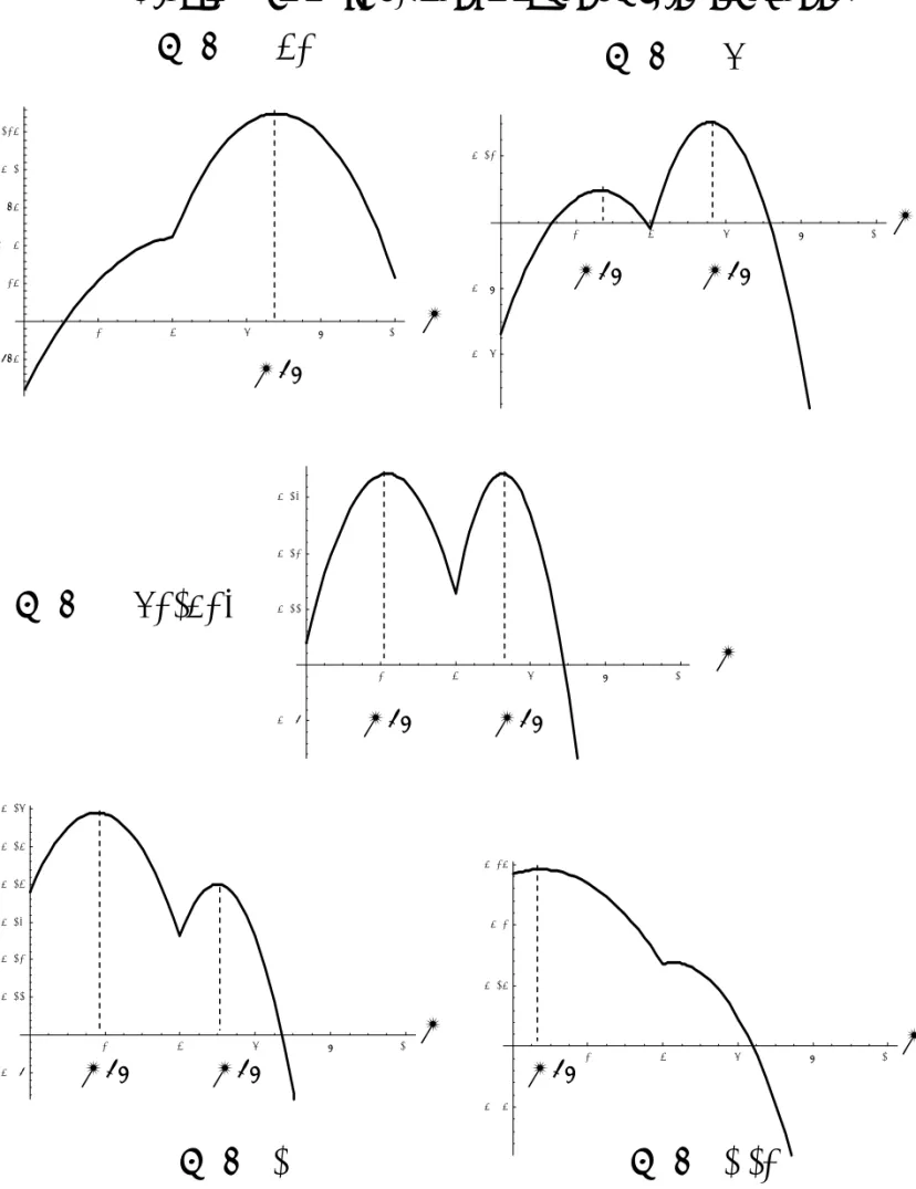
Figure 1 presents a numerical simulation with the following values of

parameters: = 2; = 0:5; = 0:17; = 0:5; = 1; w2 = 2; q0 = 0:5 and

w1 = 1:The di¤erent curves are obtained for di¤erent values of the parameter

w04. The objective function of self 1 with respect to m is drawn. The value

4_{The same type of analysis could be carried out with respect to another parameter} than w0:

w0 = 0:951856is such that the two local maxima give the same value to the

utility. For w0 smaller than this value, the optimal behavior is to give birth

to many children ( ~mT C_{) and to not invest in their education. For w}

0 higher

than this value, the optimal behavior is to have a small number of children

(mT C_{) and to invest in their quality.}

Considering self 1’s objective function, under the condition Z( ) < w2

w1+w0 <

D( ), this function of m has two local maxima: one associated with a

posi-tive investment in education (mT C_{) and one for which education cancels out}

( ~mT C_{). Therefore it is necessary to compare the utility levels obtained for}

each local maximum. UT C _{denotes the indirect utility level when q}T C _is

pos-itive and ~UT C _{the utility level when q}T C _{is zero. The following lemma shows}

that the equality UT C _{= ~U}T C _{implicitly de…nes a function V ( ) such that}

w2

w1+w0 = V ( ) , U

T C _{= ~U}T C_{:Moreover, U}T C _{> ~U}T C

, w2

w1+w0 > V ( ):

Lemma 1 Assume that Z( ) < w2

w1+w0 < D( ): The condition U T C _{> ~U}T C holds i¤: w2 w1+ w0 w0 q0 + 1 1 1= " 1 + w0 q0 1 ( ) A( ) #1= (16) > " 1 + w0 q0 1 2 #1= + w2 w1+ w0 1 1=

This inequality implicitly de…nes a function V ( ) such that

UT C > ~UT C _, w2

w1+ w0

> V ( ); (17)

and this function satis…es:

Z( ) < V ( ) < D( ):

Proof. See Appendix 2.

This lemma allows characterizing the optimal solution for w2

w1+w0 2 [Z( ); D( )] :

If w2

w1+w0 > V ( ); the optimal TC-solution is such that q

T C _{> 0: If} w2

w1+w0 <

V ( ); the optimal TC-solution is such that qT C _{= 0:}

3.3

Existence of the di¤erent regimes

This part provides a characterization of the existence of the di¤erent regimes with respect to the parameter : It is based on a technical lemma:

Lemma 2 H( ) is an increasing function of ;and when goes from

0 to 1; H( ) goes from 0 to ( q0) ( w0) (1 + 1 ) > D(1):

More-over, for every ; H( ) > Z( ):

G; Z; V _{and D are such that: 8 2 (0; 1) ;}

G( ) < Z( ) < V ( ) < D( ) and

G(1) = Z(1) = V (1) = D(1) = ( q0) ( w0)

1 + q₀ 1 2 ( w0)1

G increases with and D decreases with .

Proof. The proof results from straightforward calculations.

This lemma allows a complete characterization of the di¤erent cases.

Pa-rameters are restricted to be such that (7) holds, or w2=(w1+ w0) < H( ):

In this zone, the preceding analysis has shown that the functions G( ) and

V ( ) are the pertinent frontiers. The set of parameters can be divided into

3 sub-zones A; B and C. The following proposition gives for each zone the corresponding expressions of fertility and education. A numerical

illustra-tion (see Figure 2) is provided for the following values of parameters : = 2;

= 0:5; = 0:17; = 1; q0 = 0:5:

Proposition 4 The plan ( ; w2=(w1+ w0)) can be separated into three

zones:

Zone A = f( ; w2=(w1 + w0)); w2=(w1 + w0) < G( )g,

Zone B = f( ; w2=(w1+ w0)); G( ) < w2=(w1+ w0) < V ( )g ;

Zone C = f( ; w2=(w1+ w0)); V ( ) < w2=(w1 + w0)g.

Assuming that parameters are such that w2=(w1+ w0) < H( );

in zone A; qC _{= q}T C _{= 0 and ~m}C _{= ~m}T C_;

in zone B; qT C _{= 0; q}C _{> 0 and ~m}T C _{> m}C_;

in zone C; qT C _{> 0; q}C _{> 0 and m}T C _{< m}C_:

In zone A, the optimal behavior in both cases leads to no investment in quality. When investment in quality cancels out, both solutions are associ-ated with the same level of fertility.

In zone B, the time consistent solution leads to a higher level of fertility than the commitment solution, and to no investment in children’s quality. If self 2 could commit on a higher investment in education, self 1 would invest less in quantity.

Zone C corresponds to the developed economy with a positive investment in quality. The temporary consistent solution leads to lower investment in quantity. If self 2 could commit on a higher investment in education, self 1 would invest more in quantity.

For a given value of w2=(w1+ w0);it is possible that all three zones A; B

and C are successively reached depending on the value of :

Two cases may happen. In the case w2=(w1+ w0) < G(1);zone A appears

for close to 1; zone B for such that G( ) < w2=(w1+ w0) < V ( );zone C

appears only if there exist values of such that V ( ) < w2=(w1+w0) < H( ):

In the case w2=(w1 + w0) > G(1); only zones B and C may exist because

G( ) is always smaller than G(1) < w2=(w1 + w0): These results show that

the impact of on the investments in quality can be ambiguous for the TC

solution. Indeed, an increase of has a twofold e¤ect. For a given level of

fertility, increasing rises the investment in quality. But an increase in

also rises the investment in quantity, which has a negative impact on the investment in quality.

4

Impact of the costs of fertility and

educa-tion

This section studies how fertility and education behaviors respond to changes

of w0 and :

4.1

E¤ect of

w

w0 play a crucial role in education and fertility. An increase of w0 has a

twofold impact: …rst it increases the opportunity cost of the quantity of children; second, for a given level of fertility, it increases the …rst period income of the family. The …rst e¤ect (e¤ect on the price) is expected to dominate the second one (e¤ect on the revenue), as in the standard trade-o¤

model between consumption and leisure. Therefore, the increase of w0 is

In writing equation (6) under the form: mT C = ( ) A( )( q0) (w1+w0) w0 w2( w0) 1 q0( w0) 1+ ( ) A( )( q0)

it is straightforward that mT C is a decreasing function of w0 as the numerator

is decreasing and the denominator is increasing. Using the same argument,

mC _{given by (8) is also decreasing with respect to w}

0:Finally, when education

cancels out, equation (13) can be written again as ~ mT C = 2 _q 1 0 (w1+w0) w0 ( w0) 1+ 2 q0 1

which is decreasing with w0:

In all cases, fertility decreases with respect to w0: A change of w0 can

also result in a change of regime, and a drop in fertility. Starting from the

fertility level without education ~mT C; an increase of w0 implies a decrease

in fertility. This change of w0 may induce such a decrease in fertility that it

becomes optimal to invest in quality. At this point, there is a discontinuity in

fertility that experiences a fall between ~mT C and mT C: In the neighborhood

of the frontier value of w0;a small increase of w0 induces a great drop in

fer-tility. This jump is the consequence of the discrepancy between the objective functions of self 1 and self 2. Figure 3 gives a numerical illustration for the

following values of parameters : = 2; = 0:5; = 0:17; = 0:5; = 1;

w2 = 2; q0 = 0:5; w1 = 1:Parameters are such that for w0 = 0:951856 there

is the discontinuity in fertility.

The frontiers between the di¤erent regimes can be characterized with

re-spect to w0:They cannot be deduced from Figure 2, as the di¤erent functions

H; V and G depend on w0:The characterization is made in the plan (w0; w1):

As before, parameters are constrained in such a way that mT C _{> 0; which}

corresponds to condition (7). This constraint de…nes in the plan (w0; w1) a

zone such that w1 > WH(w0); with WH a function de…ned in Appendix (3).

The same method is used for condition (11): a function WG_(w

0) is

intro-duced, such that the condition holds i¤ w1 < WG(w0): Finally, the function

WV(w0)is introduced, such that condition (17) holds i¤ w1 < WV(w0):The

three functions WH_(w

0); WG(w0) and WV(w0) allow to obtain a

character-ization of the di¤erent regimes in the plan (w0; w1): This characterization

is equivalent to the one given in section 3.3 in the plan ; w2

w1+w0 ; but it

shows the role of w0 in the existence of the di¤erent regime.

The following proposition gives the complete characterizations of the

dif-ferent regimes in the plan (w0; w1); using the frontiers de…ned by the three

functions WH_(w

Proposition 5 It is possible to de…ne three functions WH_(w

0); WG(w0)

and WV_(w

0) that are non-decreasing functions of w0; and for all w0;

WG_(w

0) > WV(w0):

The plan (w0; w1) can be separated in three zones:

Zone A = (w0; w1) ; w1 > WG(w0) ,

Zone B = (w0; w1) ; WV(w0) < w1 < WG(w0) ;

Zone C = (w0; w1) ; w1 < WV(w0) .

Assuming that parameters are such that w1 > WH(w0);

in zone A; qC _{= q}T C _{= 0 and ~m}C _{= ~m}T C_;

in zone B; qT C = 0; qC > 0 and ~mT C > mC;

in zone C; qT C _{> 0; q}C _{> 0 and m}T C _{< m}C_:

Proof. See Appendix 3.

Zone A is obtained for a low value of w0; qC = qT C = 0 and ~mC = ~mT C.

As the opportunity cost of children is small, fertility is high and parents do not invest in quality.

In zone B; qT C = 0but qC > 0and ~mT C > mC. For an intermediate value

of w0; the TC behavior leads to no investment in quality, whereas parents

invest in quality along the commitment solution. Fertility is lower for the commitment solution.

In zone C; qT C _{and q}C _{are both positive and m}T C _{< m}C_{. For a high value}

of w0; the TC and C solutions are associated with a positive investment in

quality, and fertility is higher for the commitment solution.

A consequence of these results for the TC behavior is that fertility

ex-periences a strong discontinuity for w0 = WV

1

(w1) w0l: In the

neigh-borhood of this value wl

0, a small increase of w0 leads to a large drop in

fertility.

Figure 4 shows a numerical simulation of the di¤erent zones in the plan

(w0; w1); for the same values of parameters as Figure 3. For w1 = 1; fertility

experiences a discontinuity at the value w0 = 0:951856.

The discontinuity in the optimal strategy of self 1 is a particular feature of the model with quasi-hyperbolic discounting. In the model with exponential discounting, a change in the value of some parameter results in a continuous e¤ect on the choices of the agent. In the model with quasi-hyperbolic dis-counting, it is possible to observe jumps that are related to the non-concavity

of self one’s objective. This property introduces a qualitative di¤erence in the two models that may have important empirical consequences. If the model with quasi-hyperbolic discounting is relevant, fertility behaviors may undergo large changes for some critical values of the parameters. This may have consequences for the empirical analysis of fertility and for the dynamics of demographic transitions.

4.2

E¤ect of

The parameter is the cost of education. An increase of changes the

optimal trade-o¤ between quality and quantity. The following proposition

summarizes the e¤ect of on fertility and education.

Proposition 6 mC _{increases when the cost of education increases,}

and qC_decreases.

If is small enough, i.e. < 1=(1 ); mT C increases when the cost

of education increases, and qT C_(mT C_{) decreases. If > 1=(1 );}

mT C _{can be a non monotonic function of :}

There exists a threshold ; with > 1=(1 ); such that if < ;

qT C_(mT C_{) decreases with :}

Proof. See Appendix 4.

For the commitment solution, an increase of reduces the investment in

education, and increases fertility. This result is standard in the basic model of quantity-quality trade-o¤. For a given level of fertility, an increase of reduces the investment in education q. As q is lower, the cost of fertility decreases and fertility increases. For the TC-solution, the same e¤ect is

obtained for a small value of : But if is very high, can have a non

monotonic e¤ect.

As for w0; there exists a threshold level l such that education cancels

out for > l_{. At this point} l_{, fertility is not continuous and jumps to a}

higher value, as education falls to zero. Figures 5 and 6 show how fertility

may evolve with respect to : Figure 5 uses the preceding values for the

di¤erent parameters: = 2; = 0:17; = 0:5; = 1; q0 = 0:5; w0 = 1;

w1 = 1; w2 = 2: The threshold level from which education cancels out is

l _{= 0:516066:}

Figure 6 is an example of parameters leading to a non-monotonic

evo-lution of fertility for a high value of . = 4; = 0:28; = 0:5; = 1;

An increase of also in‡uences the existence of the di¤erent regimes. This

question is studied in the plan ( ; w2=(w1+ w0)) ;considering how the

di¤er-ent frontiers G( ) and V ( ) are modi…ed. For given, it is straightforward

from (12) that G( ) in an increasing function of : As could be expected,

the region A in which no education occurs increases with : Consequently

there is less space for regions B and C. The frontier between regions B and

C is de…ned with the function V ( ): Appendix 5 shows that V ( ) increases

with . A numerical experiment is provided in Figure 7, with the following

parameters = 2; = 0:17; = 1; q0 = 0:5, = 0:5 and = 0:7:The case

= 0:7 is presented with bold lines.

5

Conclusion

This paper has studied the quantity-quality fertility model under the as-sumption of quasi-hyperbolic discounting. The impact of the absence of self control is isolated through the comparison between the TC solution (sophis-ticated behavior) and the C solution (commitment solution). The lack of self control may have di¤erent impact on fertility in a developed economy and in a developing one. In a developed economy characterized by a positive investment in quality, the lack of self control tends to reduce fertility. In a developing economy, the lack of self-control may lead to both no investment in quality and a higher fertility rate. It is also proved that if parents cannot commit on their investment in quality, a small change of parameters may lead to a jump in fertility and education.

This paper could be extended in di¤erent directions. First, the robust-ness of the results could be studied if the model was enriched by additional assumptions: access to capital markets for the households, imperfect capital markets through borrowing constraints, collective choice within the house-hold, etc. Secondly, a technical improvement could be made by introducing more than three periods and more than two decisions.

References

[1] Robert J. Barro, (1999), "Ramsey Meets Laibson In The Neoclassical Growth Model," The Quarterly Journal of Economics, vol. 114(4), pages 1125-1152, November.

[2] Becker, G. S. and Lewis, H. G. (1973) ’Interaction between Quantity and Quality in Children’. Journal of Political Economy, 81, S279-S288.

[3] Becker, G. S. and Tomes, N. (1976) ’Child Endowments and the Quan-tity and Quality of Children’. Journal of Political Economy, 84, S143-S162.

[4] Diamond, Peter & Koszegi, Botond, (2003), "Quasi-hyperbolic discount-ing and retirement," Journal of Public Economics, vol. 87(9-10), pages 1839-1872, September.

[5] Harris, Christopher & Laibson, David, (2001), "Dynamic Choices of Hyperbolic Consumers," Econometrica, vol. 69(4), pages 935-57, July. [6] Harris, Christopher and David Laibson. (2002), "Hyperbolic

discount-ing and consumption". Mathias Dewatripont, Lars Peter Hansen, and StephenTurnovsky, editors. Advances in Economics and Econometrics: Theory and Applications, Eighth World Congress (1)258-298.

[7] Laibson, David, (1997), "Golden Eggs and Hyperbolic Discounting," The Quarterly Journal of Economics, MIT Press, vol. 112(2), pages 443-77, May.

[8] Loewenstein, George & Thaler, Richard H, (1989). "Intertemporal Choice," Journal of Economic Perspectives, vol. 3(4), pages 181-93, Fall. [9] Salanié, Francois & Treich, Nicolas, 2006. "Over-savings and hyperbolic discounting," European Economic Review, Elsevier, vol. 50(6), pages 1557-1570, August.

[10] Wrede Matthias (2009) Hyperbolic discounting and fertility. Journal of Population Economics, Online publication date: 9-Oct-2009.

[11] Wigniolle Bertrand (2010), "Hyperbolic discounting and discontinuous savings strategies", mimeo, University of Paris 1.

6

Appendixes

6.1

Appendix 1

The comparison between mT Cand mC is made in the text. In the case < 1;

the comparison between qC_(mC_{)and q}T C_(mT C_{)is simple and is made in the}

text. It remains to compare qC_(mC_{)and q}T C_(mT C_{)when > 1:}

qT C(mT C) + qo = ( = ) w2 mT C + q0 1 + ( ) 1 and qC(mC) + qo = ( = ) w2 mC + q0 1 + ( ) 1 From (6), is obtained: w2 mT C + q0 = ( ) A( )B [ q0(w1+ w0) + w2 w0] ( ) A( )B (w1+ w0) w2 (18) From (8), is obtained: w2 mC + q0 = ( ) A(1)B [ q0(w1+ w0) + w2 w0] ( ) A(1)B (w1+ w0) w2 (19) As A(1) = 1 + 1 _{; it follows:} qT C(mT C) + qo < qC(mC) + qo , ( ) 1 + ( ) 1 A( ) ( ) A( )B (w1+ w0) w2 < 1 ( ) A(1)B (w1+ w0) w2 (20) After rearranging and using the expression (4) of A( ); it is possible to write this inequality: 0 < B (w1+ w0) w2f ( ) (21) with f ( ) 1+ 1 + 1 1 1

Firstly the inequality (21) is studied in a neighborhood of = 1: In

setting x = ; a function g is introduced such that:

g(x)

1+x 1

x1= _+x 1 1

1 x = f ( )

The limit of g when x tends toward 1 is equal to the limit of f in = 1:

De…ning a function h(x) such that:

h(x) 1 + x

1

this limit is equal to h0_{(1): Taking the derivative of the logarithm of h in} x = 1; it is obtained: h0(1) = h0(1)=h(1) = 1 1 + 1 1 + 1 1 + 1 = 1 1 + 1

Thus, with = 1; (21) becomes:

0 < B (w1+ w0)

w2

1 + 1

which is satis…ed as it corresponds to (9) with = 1: It is then proved that

qT C _{< q}C _{in a neighborhood of = 1:}

Secondly, the inequality (21) is studied for a low value of : When tends

toward 0; f ( ) tends to be in…nite, the inequality (21) cannot be satis…ed,

and qT C _{> q}C_{: close to 0 is not possible as it implies negative values for}

mT Cand mC:The smallest possible value of corresponds to the constraint

(7) ensuring mT C _{> 0: When tends to this value, the left-hand side of (20)}

tends to be in…nite. Thus, when is low enough, (21) cannot be satis…ed,

and qT C > qC:

6.2

Appendix 2

In this appendix, a new notation x is introduced for the expression w2

w1+w0:

Assume that Z( ) < x < D( ): The equality UT C _{= ~U}T C _{implicitly de…nes}

x as a function of : f (x; ) = 0 with f (x; ) 1 UT C U~T C 1 (w1+ w0)1 1= = x w0 q0 + 1 1 1= " 1 + w0 q0 1 ( ) A( ) #1= " 1 + w0 q0 1 2 #1= x1 1=

First, it is proved that @f =@x > 0: The condition @f =@x > 0 is equivalent to: w0 q0 x w0 q0 + 1 1= " 1 + w0 q0 1 ( ) A( ) #1= > x 1=

which is equivalent to x > 1 w0 q0 ( ) + w0 q0 [A( ) 1] ( )

From this inequality, as by assumption x > Z( ); if Z( ) > ( ); the

property x > ( ) will be satis…ed and @f =@x > 0.

Z( ) > ( )is equivalent to: w0 q0 A( ) 1 ( ) 1 + w0 q0 ( ) 1 1 + ( ) 1 A( ) > 0

From the de…nition of A( ); A( ) > 1 + ( ) 1

, 1 + 1 1 _>

1 + ( ) 1 _{which is true for < 1:}

Finally the property @f =@x > 0 is proved.

The next step is to prove that f (Z( ); ) < 0 and f (D( ); ) > 0: These two inequalities with the property @f =@x > 0 will ensure the existence and

uniqueness of x as a function V ( ) of :

After tedious calculations, it is possible to write f (Z( ); ) < 0 under the form 1 + w0 q0 1 2 + 1 1 + 1 1 < " 1 + w0 q0 1 2 #1= " 1 + w0 q0 1 2 + 1 1 + 1 #1 1=

The following notations are introduced:

a = w0 q0 1 2 y( ) = + 1 1 + 1

It is possible to write the preceding inequality:

[1 + ay( ) 1]

[1 + ay( ) ] 1 < 1 + a (22)

As a function of y; the expression

[1 + ay 1_]

[1 + ay ] 1

is strictly increasing when y goes from 0 to 1; and is equal to 1 + a for y = 1: By these two properties, it is proved that (22) is satis…ed.

The condition f (D( ); ) > 0 can be written after some calculations " 1 + w0 q0 1 1 + 1 #1 1= " 1 + w0 q0 1 ( + 1 ₎ (1 + 1 ₎ 1 #1= > 1 + w0 q0 1 + 1

The following notations are introduced:

b = w0

q0

1

= 1 + 1

= + 1

By de…nition, with a strict inequality for < 1: It is possible to write

the preceding inequality:

1 + b ₁ > (1 + b )

(1 + b ) 1 (23)

De…ning the function g:

g( ) = 1 + b ₁ (1 + b )

(1 + b ) 1

it is easy to check that it is strictly decreasing for _{2 [0; ] ; with g( ) = 0:}

Therefore, it is proved that (23) is satis…ed, and f (D( ); ) > 0.

6.3

Appendix 3

Condition (11) can be written under a condition on w0and w1:The inequality

w2 w1+w0 > G( ) is equivalent to: w1 < w2 q0 1 w0+ w2( w0) ( q0) ( ) (w0)

The right-hand side member of this inequality is a function of w0 such that:

if w2

q0 > 1; is strictly increasing; if

w2

q0 < 1; is U-shaped, …rst

decreasing and then increasing. As w1 cannot be negative, the negative part

of does not play any role. The function WG _{is de…ned a}

WG(w0) = maxf (w0); 0g

By de…nition, either WG(w0) is strictly increasing, or it is …rst equal to 0;

and then strictly increasing.

For condition (10), the inequality w2

w1+w0 > Z( )is equivalent to: w1 < w2 q0 1 w0+ w2( w0) ( q0) 1 + 1 + 1 #(w0)

As for the preceding example, a function WZ _{is de…ned as}

WZ(w0) = maxf#(w0); 0g

By de…nition, WZ(0) = 0; either WZ(w0) is strictly increasing, or it is …rst

equal to 0; and then strictly increasing.

For condition (14), the inequality w2

w1+w0 < D( ) is equivalent to: w1 > w2 q0 1 w0+ w2( w0) ( q0) (w0)

As for the preceding examples, a function WD is de…ned as

WD(w0) = maxf (w0); 0g

By de…nition, WD_{(0) = 0; either W}Z_(w

0) is strictly increasing, or it is …rst

equal to 0; and then strictly increasing. Finally condition (7) can be written:

w1 >

w2( w0)

( q0) ( )

(1 + 1 ) 1

1 + 1 1 w0 (w0)

As for the preceding examples, a function WH _{is de…ned as}

WH(w0) = maxf (w0); 0g

By de…nition, WH_(w

Lemma 4 with Appendix 2 allow to de…ne a function V ( ) such that

w2

w1+w0 = V ( ) , U

T C _{= ~U}T C_{: This function V ( ) depends on di¤erent}

parameters of the model including w0;but does not depend on w1:Therefore,

it is clear that it can be expressed under the form:

w1 =

w2

V ( ) w0

A function WV _{is de…ned as:}

WV(w0) = max

w2

V ( ) w0; 0

As Z( ) < V ( ) < D( ); it implies that: WD(w0) < WV(w0) < WZ(w0):

To …nd how WV_(w

0) evolves with w0; it is useful to come back to the

de…nition. When w1 = WV(w0)is positive, the function is implicitly de…ned

by the relation UT C U~T C = 0: The derivative is implicitly given by:

dWV_(w 0) dw0 = @(UT C _U~T C₎ @w0 @(UT C _U~T C₎ @w1 If@(U T C _U~T C₎

@w0 6= 0; it will prove that W

V_(w

0)is monotonic. As WD(w0) <

WV(w0) < WZ(w0); with WD(w0) and WZ(w0) two increasing functions

tending to +1 when w0 ! +1; the only possibility will be that WV(w0)is

monotonically increasing.

It is possible to prove that @(U

T C _U~T C₎

@w0 > 0: U

T C _{is the maximum value}

of self 1’s objective function when qT C_{(m) > 0: ~U}T C _{is the maximum value of}

self 1’s objective function when qT C_{(m) = 0:The derivatives can be obtained}

using the envelope theorem:

@UT C @w0 = (1 mT C) w1+ w0(1 mT C) 1 @ ~UT C @w0 = (1 m~T C) w1+ w0(1 m~T C) 1 As > 1; the function x [w1+ w0x] 1

is an increasing function of x; as its logarithmic derivative is

w1+ ( 1)w0x

Consequently, the function (1 m) [w1+ w0(1 m)]

1

is a decreasing

function of m: As ~mT C > mT C; it is obtained that,

@UT C

@w0

> @ ~U

T C

@w0

which implies that the function WV_(w

0)is increasing.

6.4

Appendix 4

From (8), mC _{can be written:}

mC = x( ) (w1+ w0)

w2

q0

1 + w0x( )

with x( ) ( ) q₀ 1( w0) ( 1+ s):Taking the derivative of mC with

respect to ; it is obtained that the sign of this derivative is the sign of the expression: x0( ) (w1+ w0) + w2 2_q 0 [1 + w0x( )] x( ) (w1+ w0) w2 q0 [ w0x0( )] = x0( ) (w1+ w0) + w0 w2 q0 + w2 2_q 0 [1 + w0x( )] > 0

Thus, mC _{is an increasing function of :}

From (3), the quality level q is such that:

q0 + q( + ) =

w2

mC

If increases, as mC _{increases, q must decrease.}

From (6), the time-consistent solution can be written:

mT C = y( ) (w1+ w0)

w2

q0

1 + w0y( )

with y( ) ( ) q₀ 1( w0) 1A( ): If y0( ) > 0; it is known from the

preceding calculation that mT C increases with : Therefore, it remains to

check if 1_{A( ) increases with : After some calculations, it is obtained}

that

d ln [ 1_{A( )]}

d = ( 1)

1 [ (1 ) 1] 1 1

If (1 ) < 1; y0_{( ) > 0 and m}T C _{increases with : If (1 ) > 1; it is}

not possible to achieve a general conclusion.

Assuming that mT C _{increases with ; from (2), the quality level q is such}

that:

q0 + q( + ( ) ) = ( )

w2

mT C

If increases, as mT C _{increases, q must decrease.}

Considering now qT C(mT C); Appendix 1 has shown that

qT C(mT C) + qo = ( = ) w2 mT C + q0 1 + ( ) 1 or qT C(mT C) + qo = ( ) [ q0(w1+ w0) + w2 w0] + ( ) ( ) A( )B ( ) A( )B (w1+ w0) w2

It is easy to check that the …rst term

( ) [ q0(w1+ w0) + w2 w0]

+ ( ) =

( ) q0(w1+ w0) + w2 w0

1_{+ ( )}

is a decreasing function of as > 1:

De…ning z( ) = ( ) A( )B; the second term can be written

z( )

z( ) (w1+ w0) w2

This is a decreasing function with respect to z( ): Therefore, if z( ) increases

with ; it will be obtained that qT C_(mT C_{)is a decreasing function of :}

z( ) can be written:

z( ) = ( ) q0

w0

+ 1

( + ) 1

The sign of z0_{( )=z( ) is given by the sign of:}

2 1₊ 1 2_{(1 ) + (2 ) + +} 2 2 1

A su¢ cient condition to have z0_{( ) > 0is that} 2_{(1 )+(2 ) + > 0:}

Considering this second degree equation in ; the property z0_{( ) > 0will hold}

if

< 2 +

p

4 3 2

2(1 )

6.5

Appendix 5

This appendix proves that V ( ) increases with : This function has been

de…ned in Appendix 2 as the solution x implicitly de…ned by the equation:

f (x; ) = 0 with x = w2

w1+w0 and

f (x; ) = 1 UT C U~T C 1

(w1+ w0)1 1=

From this de…nition, it appears that @V ( ) @ = @f @ @f @x

In Appendix 2, it was shown that @f_@x > 0: It remains to prove that @f_@ < 0;

which is equivalent to prove that: @(U

T C _U~T C₎

@ < 0: U

T C _{is the maximum}

value of self 1’s objective function when qT C_{(m) > 0: ~U}T C _{is the maximum}

value of self 1’s objective function when qT C_{(m) = 0: The derivatives can be}

obtained using the envelope theorem:

@UT C @w0 = mT CqT C w2 mT CqT C) 1 @ ~UT C @w0 = 0 Therefore, @(U T C _U~T C₎

2 4 6 8 10 4.975 5.025 5.05 5.075 5.1 5.125 2 4 6 8 10 5.06 5.08 5.12 2 4 6 8 10 5.09 5.11 5.12 5.13 5.14 5.15 5.16 2 4 6 8 10 5.05 5.15 5.2 5.25

Figure 1: self 1’s objective function with respect to

m

m

m

m

_m

w

= 0.75

_w

_{= 0.9}

w

= 1

w

= 1.15

w

= 0.951856

m

m

_m

m

_m

m

m

_m

~

~

~

~

m

0 . 2 0 . 4 0 . 6 0 . 8 1 0 . 5 1 1 . 5 2

E

w

+ w

w

H(

_E

)

G(

_E

)

V(

_E

)

Zone A

Zone B

Zone C

Figure 2

ı = 2, IJ = 0.5, ij = 0.17, į = 1, q

= 0.5

ı = 2, IJ = 0.5, ij = 0.17, į = 1, q

= 0.5, w

= 2, w

= 1

m

m

0.2 0.4 0.6 0.8 1 1.2 1.4 0.5 1 1.5 2 2.5 3

Figure 4

w

W

W

W

w

Zone A

_{Zone B}

Zone C

w

ı = 2, IJ = 0.5, ij = 0.17, į = 1, q

= 0.5, w

= 2

m

m

ı = 2, E = 0.5, ij = 0.17, į = 1, q

= 0.5, w

= 1, w

= 2, w

= 1

W

W

m

m

Figure 6

ı = 4, E = 0.5, ij = 0.28, į = 1, q

= 1.5, w

= 2, w

= 1

IJ = 0.5 and IJ = 0.7, ı = 2, ij = 0.17, į = 1, q

= 0.5

H(

_E

)

V(

_E

)

G(

_E

)

Zone C

Zone B

Zone A

w

+ w

w