HAL Id: halshs-01318131
https://halshs.archives-ouvertes.fr/halshs-01318131
Submitted on 19 May 2016HAL is a multi-disciplinary open access archive for the deposit and dissemination of sci-entific research documents, whether they are pub-lished or not. The documents may come from teaching and research institutions in France or abroad, or from public or private research centers.
L’archive ouverte pluridisciplinaire HAL, est destinée au dépôt et à la diffusion de documents scientifiques de niveau recherche, publiés ou non, émanant des établissements d’enseignement et de recherche français ou étrangers, des laboratoires publics ou privés.
What does it take to grow out of recession? An
error-correction approach towards growth convergence
of European and transition countries
Olivier Damette, Mathilde Maurel, Michael A. Stemmer
To cite this version:
Olivier Damette, Mathilde Maurel, Michael A. Stemmer. What does it take to grow out of recession? An error-correction approach towards growth convergence of European and transition countries. 2016. �halshs-01318131�
Documents de Travail du
Centre d’Economie de la Sorbonne
What does it take to grow out of recession? An error-correction approach towards growth convergence of European and transition countries
Olivier DAMETTE, Mathilde MAUREL, Michael A. STEMMER
What does it take to grow out of recession? An error-correction
approach towards growth convergence of European and
transition countries
by
Olivier Damettea, Mathilde Maurelb , Michael A. Stemmerc
April, 2016
Abstract
Consequences from the subsiding 2008 financial crisis on long-run economic growth are widely debated. Existing literature on previous recessions, such as Cerra and Saxena (2008), emphasizes the long-term loss inflicted on per capita GDP levels. This paper concentrates on typical business cycles in advanced European and transition countries and assumes that lower than normal growth during recessions is followed by a recovery period with above normal growth until the economy reaches its pre-crisis level. The objective is to assess the capacity to rebound, the speed of convergence towards a normal growth path as well as potential nonlinearities. Through exploiting the cointegration relationships among variables in long-run growth regressions and by employing a variety of panel error-correction models, results show a strong evidence of error-correction and different linear speed in the convergence process with the transition economies outpacing Western European countries. Our analysis is further extended into a Panel Smooth Transition Error-Correction Model (PSTR-ECM) to account for different regimes in convergence patterns according to a selection of transition variables. Whereas the velocity of convergence for European core countries exhibits a nonlinear pattern and differs with respect to price and flexibility, transition countries remain linear in their return to the growth trend. Ultimately, our results suggest that internal adjustments remain the key factors for both European and transition countries to recover from negative economic growth shocks.
Keywords: Economic growth, business cycles, transition economies, error-correction models, panel cointegration, smooth-transition models
JEL Classification Codes: C23, C50, E32, F43, O40
We are grateful to Michael Funke, our discussant Michael Graff at the Makroökonomik und Konjunktur Workshop at the ifo Dresden and Valerio Scalone for their helpful comments. Remarks from participants in seminars at Université Paris 1 Panthéon-Sorbonne, the Paris School of Economics, Université de Lorraine, the Conference on the Imperative of Economic Growth in the Eurozone in Brno and the Annual Macroeconometric Workshop at the DIW have been highly appreciated. All remaining errors remain our own.
a Université de Lorraine, BETA-CNRS and LEF INRA Agroparitech, and IXXI – “Complex Systems Institute” –
ENS Lyon, email: olivier.damette@univ-lorraine.fr;
b Correspondance to: CES, Université Paris 1 Panthéon-Sorbonne, Fondation pour les Études et Recherches sur
le Développement International (FERDI), email: mathilde.maurel@univ-paris1.fr;
“… a key fact is that recessions are followed by rebounds. Indeed, if periods of lower-than-normal growth were not followed by periods of higher-than-normal growth, the unemployment rate would never return to normal.”
Council of Economic Advisors of President Obama, February 28th, 2009
1. Introduction
The consequences of the subsiding 2008-09 financial crisis on long-run economic growth and the policy implications that can be drawn from it have become widely debated. For many, the recovery in both the United States and Europe has been unusually sluggish and has been characterized by persistently high unemployment rates. (Bordo and Haubrich, 2012; Beyer and Stemmer, 2016). The 2012 conference of the Federal Reserve Bank of Boston on “Long-Term Effects of the Great Recession” was, for instance, exclusively devoted to this topic. In the accompanying conference issue, Papell and Prodan (2012) find evidence of a full recovery in the US not until late 2016 but no lasting effect on long-term potential GDP.
Yet, this has not always been the case. Covering crises earlier and elsewhere, Cerra and Saxena (2005), for instance, provide evidence that the banking crisis in Sweden in the early nineties explains why the country has incurred a permanent loss in its long term GDP per capita level. Coricelli and Maurel (2011), by focusing on transition countries which have switched from planned to market economies and experienced severe transitional recessions, show that the transitional recession is particularly deep with long term consequences, and argue that the capacity to rebound, proxied by the depth and length of the crisis, depends foremost on the quality of the financial institutions and trade liberalization.
However, studies on financial crises cover in many respects only the extreme versions of cyclical downturns and recessions. In this work we move beyond the mere focus on economic crises and concentrate instead on typical business cycle swings, which may have a permanent effect on long-term average growth. As an assumption we follow the conventional view that lower than normal growth during a recession is followed by a recovery period with above normal growth rates. Once the economy reaches its potential output (and full employment), growth continues to follow its normal equilibrium trend. Consequently, the primary objective of this paper is first to assess whether a convergence towards this normal growth path exists and at what speed such a return is happening. Second, we further analyze potential non-linearity of this convergence process and control for factors impacting such a behavior. In contrast to a majority of the literature, which is concentrating on the US, we focus in the following analysis on European core countries and the Eastern European transition economies. Our analysis is structured as follows: initially, we test for time series properties and estimate long-term (cointegration vector) growth models to check for long-run relationships and growth determinants of our country samples. As a next step linear error-correction models are employed to assess potential differences in adjustment velocity towards
the long-run growth trend, thereby also controlling carefully for slope heterogeneity and cross-sectional dependence among countries. In order to account for potential non-linearity and different regimes in growth convergence behavior, we additionally estimate nonlinear Panel Smooth Threshold Regression-Error Correction Models, which allow for a determination of different regimes according to a selection of transition variables.
Results show that the error-correction terms from the linear models, i.e. the speed of convergence towards normal growth, are highly significant and that they are larger for transition countries. Moreover, as for non-linearity in the process found, convergence to the equilibrium varies only for EU-core countries with respect to the degree of price and wage flexibility. Typically, the more flexible an advanced EU country is, the faster the catching-up process it will experience. Moreover, not flexible enough countries may fail to converge to their long run average output growth.
The rest of the paper is structured as follows: Section 2 presents previous literature on the topic and sets the theoretical underpinning for the analysis thereafter. Subsequently in Section 3, the overall estimation design is briefly outlined and thereafter data is explained. Section 5 focuses on the technical specificities of the linear estimations where part one covers the dynamic long-term growth models including the undertaken tests for unit roots and co-integration in the variables as well as error-correction models. The analysis of non-linearity by describing in detail estimations with the Panel Smooth Threshold Regression-Error Correction Model follows in the penultimate part. Eventually Section 7 concludes.
2. Related Literature and Theoretical Underpinning
From 2008 to 2012 the Great Recession as well as the European debt crisis revealed the different adjustment strategies to a crisis. EMU membership prohibited depreciation as a quick remedy for the adjustment of unit labour costs to regain international competitiveness. The loss of independent monetary policy made price and wage adjustments necessary, which magnified the recession and provoked different policy responses. Whereas Ireland (like the Baltic countries and Bulgaria) embarked on drastic reforms in the private and public sector, in Greece political resistance delayed reforms and paved the way to the recent political crisis. This situation is reminiscent of a discussion during the world economic crisis in the 1930s. Whereas Keynes (1936) called for a depreciation to provide a short-term growth impulse, Hayek (1937) stressed the need of price and wage adjustment. While the former emphasised the need for a timely anti-cyclical macroeconomic impulse, the latter believed in the self-stabilizing forces of the market. In the same vein, Mundell (1961) assumes that countries need to preserve the exchange rate as an adjustment mechanism, even more if prices and wages are not flexible, while Hayek (1937) and Schumpeter (1911) insist on declining prices and wages as the prerequisites for a robust recovery after a crisis. According to them, whatever the policy needed, there is no need to make a strong distinction between the long run and the short run growth.
In contrast to those historical insights, the most recent literature on growth dynamics after a negative economic shock focuses on the detection of depth and length of a recession or crisis as well as the associated capacity to rebound.1 As documented by Kim and Nelson (1999), US recessions were usually followed by periods of high growth. High recovery periods have also been behind several other papers that find evidence of trend stationarity in GDP, such as Campbell and Mankiw (1987) or Cheung and Chinn (1999)2. More recently, Cerra and Saxena (2008) examined a variety of country groups and found varying degrees of persistence of output loss following different financial and socioeconomic crises. The argue that most of the time, crisis are not neutral on long run average growth, and the return to the latter depends upon a range of institutional features. Papell and Prodan (2012) reach a different conclusion. They analyse the length and structure of slumps, defined as a contraction and part of an expansion until the economy reaches its long-run growth rate, across a cross-section of several countries. They find that most recessions associated with financial crises in advanced countries do not cause permanent reductions in potential GDP. The situation is different for emerging countries where potential GDP is only restored in two out of six cases analysed. Beyond the divide developed versus emerging countries, Coricelli and Maurel (2011) demonstrate that more flexible financial institutions diminish the length and depth of crisis. They highlight the importance of reform complementarity, particularly in financial sector reform.
Another complementary strand of research focuses on explicit policy measures and country characteristics that exert influence on a recovery and its persistence. Bicaba et al. (2014), for example, focus on policy measures that influence stability periods between financial crises. Cerra et al. (2013) investigate macroeconomic policies that can influence the speed of recovery and mitigate the persistence of such shocks for different groups of industrialized and developing countries. Monetary expansion is thus a powerful tool in industrialized countries, yet only to rebound from recession and not during regular expansion years. Expansionary fiscal policy is found to have a positive impact for recovery in both industrialized and non-Sub-Saharan countries. Floating exchange rate regimes perform best in facilitating a growth rebound from recession and are also the preferred regime for industrialized countries to support recoveries. The opposite holds for developing countries, where a fixed regime is associated with highest rates of growth over an entire expansion. During recovery years, real appreciation deteriorates growth perspectives, impacting in particular developing countries. A clear distinction between the short and the long run was formalised in the nineties, where endogenous growth theorists show (both at the theoretical and empirical level) that there is a relation between short-term economic instability and long-run growth. According to Aghion and Saint-Paul (1993), this relation can be positive or negative, depending on whether the
1 The separate emphasis on crisis on the one hand and long-run growth on the other reflects a strong tradition
among macroeconomists, which consists in studying business cycles and long-term growth as two separate phenomena. For business cycle theorists, long-term growth is a fundamentally exogenous trend, while for growth theorists, short-term shocks are neutral on the long-run growth rate of the economy.
2 Such high growth recoveries for the US were particularly observed before the Great Moderation. Camacho et
al. (2009), however, observe since 1984 a loss of this so-called “plucking effect“ with the effect of recessions becoming more permanent.
activity that generates growth in productivity is a complement or a substitute to production. For Aghion and Saint Paul (1991), they are substitutes, which implies that a larger amplitude of business cycle fluctuations has a positive effect on long run. For Stadler (1990) and Martin and Rogers (2000), they are complementary: if growth is generated via learning by doing, a negative correlation between short and long run growth will hold, particularly in developing and emerging countries. In a similar vein, Comin and Gertler (2006) examine medium-term business cycles in the US post-war period, which are found to be more variable and persistent than conventional cycles. They find that fluctuations feature significant procyclical movements in technological change with productivity swings as a central element to the persistence of cycle fluctuations. Bianchi and Kung (2014) approach the link between business cycle shocks and long-run growth through a medium-sized DSGE framework. Apart from knowledge accumulation which links business cycle shocks and long-run growth, shocks to the marginal efficiency of investment help to explain a large share in overall macroeconomic volatility. This debate finds an echo in Fatas and Mihov (2006), who argue in a slightly different policy setting that there are two forces at work: fiscal discretion, which should reduce volatility, and responsiveness of fiscal policy, which might amplify the business cycle. At the empirical level and for the sample of 48 American states, they show that a more restrictive fiscal policy leads to less volatility in output.3
The recent work by Kocenda et al. (2013) is one of the most recent empirical papers belonging to this tradition, by disentangling long-term and short-term effects of exchange rate flexibility on growth and arguing that short run growth can be painful in the long run. On a panel of 60 emerging and developing countries the authors find that exchange rate adjustments stimulate growth in the short-term, but hamper it on the long run. Confirming the results of Maurel and Schnabl (2012), long-term growth should therefore be achieved via price and wage flexibility and stable exchange rates. Moreover, monetary expansion and depreciation as a recovery strategy from a crisis may bring short-term relief, but long-term pain.
This paper aims to contribute to this debate by initially analysing convergence speeds towards the long-term growth trend via long-run growth regressions and panel error-correction models. It thus adds some profound empirical evidence to the recent theoretical attempts of Bianchi and Kung (2014) of studying economic growth and business cycles in a more unified setting within a European context. It also contributes to the more general discussion on whether recessions have exerted a more lasting effect on long-term output during recent decades. By further assessing the non-linearity of factors that drive economic growth along business cycles and demonstrating that price flexibility affects the speed of growth convergence processes, it also blends well with the recent discussion initiated by Blanchard (2014), who emphasizes the importance of accounting for nonlinearities in the growth process, particularly in light of the recent crisis period. To our knowledge of the existing literature, we are the first to analyse the non-linearity in the present context.
3 If we consider fiscal policy as a driver of the business cycle, this result can be interpreted as evidence that fiscal
3. Estimation Design
Our empirical analysis begins by estimating endogenous long-term growth models in order to single out drivers of economic growth in the long run4. This behavior hails from nonstationary
variables, which form, if cointegrated, long-run equilibrium relationships. Hence in this paper, we set the following basic growth model:
𝑦!,! = 𝛼! + 𝛽!𝑇!+ 𝛽!𝑋′!,!+ 𝑍𝜖!,!, (1)
where 𝑦!,! is the endogenous variable that is the growth proxy, 𝑇! is a time trend, 𝑋′!,! is the vector of all long-run growth drivers (supposedly cointegrated) variables, and the vector 𝑍 comprises all exogenous variables that are not cointegrated.
For this purpose, we employ a number of estimators, which are able to cope with non-stationarity of variables (and unobserved processes) and also potential cross-sectional correlation across panel units (countries). If these issues are not properly accounted for, spurious regressions and misspecification problems may arise. The biasedness of the standard two-way fixed-effects estimator in the presence of non-stationary variables is well known. Two homogeneous estimators we first employ, the FMOLS and DOLS, which were introduced by Pedroni (2000), are able to cope with this problem and have been used throughout the literature (e.g. Kao and Chiang, 2000)5. We further introduce the CCEMG estimator developed by Pesaran (2006), which was extended to nonstationary variables in Kapetanios et al. (2011), and the alternative AMG estimator recently developed by Bond and Eberhardt (2009) and Eberhardt and Teal (2010) as a robustness check. These novel heterogeneous estimators will be further compared with the MG estimator of Pesaran and Smith (1995), which does not allow for cross-sectional correlation in the data.
We subsequently estimate linear error-correction models, in which the residuals from the previous long-run regressions serve as error-correction terms to examine convergence behavior in more detail. As recently well explained by Eberhardt and Presbitero (2015), employing an error correction model (ECM) representation in macro panels offers three advantages over static models and restricted dynamic specifications: (i) readily distinguishing short-run from long-run behaviours; (ii) investigating the error correction term and deducing the speed of adjustment for the economy to the long-run equilibrium; and (iii) testing for
4 Note that the use of the term ‘long run’ for our purpose is considered as an econometric rather than a
macroeconomic definition. The econometric definition encompasses the notion of persistency in the evolution of output – a long-run equilibrium – which may also entail firm-level productivity analysis in panels à la, for instance, Blundell and Bond (2000) over a couple of years. The macroeconometric literature usually attempts the same through long-run growth models and error-correction specifications as employed here. The long run thus refers to the range of years in the sample, rather than some macroeconomic principle extending over several generations.
5 Abbreviations for estimators hereafter: 2FE, 2-way Fixed-Effects; FMOLS, Fully Modified Ordinary Least
Squares; DOLS, Dynamic Ordinary Least Squares (Kao and Chiang, 2000); MG, Mean Group estimator (Pesaran and Smith, 1995); CCEMG, Common Correlated Effects Mean Group estimator (Pesaran, 2006); AMG, Augmented Mean Group estimator (Bond and Eberhardt, 2009; Eberhardt and Teal, 2010); PSTR, Panel Smooth Transition Regression model (González et al., 2005).
cointegration in the ECM by closer investigating the statistical significance of the error term. As an additional check, we again employ the MG, CCEMG, and AMG estimators from the previous estimation step.
Moreover, we consider non-linearity in the convergence process through the estimation of PSTR models following González et al. (2005), including as before the residuals as error-correction terms from the long-run growth equation estimations. All aforementioned estimators will be briefly explained throughout the paper in order of appearance. Note that we always estimate both subsamples separately to account for a different economic structure and economic development in both country blocks.
4. Data
The selection of growth determinants is based on the theory and empirical results laid out in the relevant growth literature. Even though Durlauf et al. (2005) have identified 140 growth regressors, the number of growth determinants in our equations, however, has been kept rather limited due to several reasons. A more parsimonious approach is advocated by Ciccone and Jarocinski (2010) and Moral-Benito (2012)6. They find that the fewer variables are included in the regressions, the less sensitive are results. Another reason is a limitation in data availability for the Eastern European transition countries. Moreover, Durlauf et al. (2008) find consistent significance for canonical neoclassical growth variables independent of the underlying growth theory followed.
We include the investment to output ratio, which is a typical Solow-type determinant and has been found to have a positive effect on economic growth (see e.g. DeLong and Summers, 1991; Sala-i-Martin, 1997). It represents the increasing relationship between capital accumulation, i.e. investment, and economic growth. We further employ the size of the labor force, defined here as the amount of people in employment compared to overall population (see e.g. Aghion and Howitt, 1992). In their endogenous theory growth benefits from a larger scale in the population for inventing new products and production techniques. Trade integration in terms of exports and imports as a share of GDP contributes to economic growth through increased opportunities for profitable investments (Levine and Renelt, 1992). Government consumption as a ratio to GDP represents distortional effects through taxation or government expenditure and has thus a negative impact on growth (Barro, 1997; Sachs and Warner, 1995). Average inflation, constructed as the average quarterly year-on-year changes of the consumer price index, controls for (detrimental) growth effects originating in macroeconomic instability (Bruno and Easterly, 1998). We also tried other usually employed variables such as the domestic credit to GDP ratio as a measure of financial development, which, however, does not turn out to be significant.
6 The authors use Bayesian averaging techniques to address both model uncertainty and endogeneity issues when
We use an original dataset of quarterly frequency that is partly borrowed from Kocenda et al. (2013) and has been extended to include the recent crisis. For most of the series, it covers a period from 1995Q1 to 2010Q4, thus the panel is unbalanced across countries. The sample coverage starts in 1995 because we want to exclude the beginning of the 1990s. For most of the Central, Eastern and Southeastern European countries the early nineties implied a transition pattern different from the business cycles framework in normal market economies, which is used in this paper. As this paper wants to single out different long-term drivers for economic growth and analyze convergence behavior of Eastern European and transition countries, the original dataset includes 15 European core countries (henceforth EU-core) and 15 Eastern European transition countries plus Turkey7. For some countries certain series were not available on a quarterly frequency and have therefore been linearly interpolated from annual data8. Detailed descriptive statistics of the data can be found in the Appendix.
The data come from the IMF’s International Financial Statistics. Missing or inconsistent data have been completed and crosschecked with national statistics, mainly at national central banks. Series used in estimations were, where necessary, seasonally adjusted9. Quarterly real GDP growth rates and inflation rates are calculated as year-over-year quarterly growth rates to filter out seasonal patterns and lower the erratic volatility of the series (𝑥!" = 𝑙𝑛 𝑋!,! − 𝑙𝑛 𝑋!,!!! ). The measure of quarterly de facto exchange rate flexibility and, in an analogue manner, of changes in the producer price index (PPI) as a measure for price and wage flexibility are computed as the quarterly arithmetic average of monthly percent exchange rate changes10. The exchange rate variable is calculated against the euro (the Deutsch mark before 1999) or the dollar, depending on the respective anchor currency. Once a country has entered the EMU the proxy for exchange rate flexibility is set to zero (see Kocenda et al., 2013). Before embarking on the results section with the estimation of the long-run relationships, we test for stationarity of the included variables via several panel unit-root tests and need to confirm whether our variables are indeed cointegrated. We further control for cross-sectional dependence among the countries in our subsamples.
7 EU-core countries: Austria, Belgium, Denmark, Finland, France, Germany, Greece, Ireland, Italy,
Luxembourg, Netherlands, Portugal, Spain, Sweden, United Kingdom
Transition countries: Albania, Bosnia-Herzegovina, Bulgaria, Croatia, Czech Republic, Estonia, Hungary, Latvia, Lithuania, Macedonia, Poland, Romania, Slovak Republic, Slovenia, Serbia, Turkey
8 Data on real GDP and government consumption for Albania and Bosnia-Herzegovina have been linearly
interpolated from annual WDI data.
9 For seasonal adjustment the X12-ARIMA package provided by the US Census Bureau was used.
10 The quarterly arithmetic average (μ) has been introduced by Ghosh et al. (2003) and combined with the
standard deviation of quarterly percent exchange rate changes of the respective quarter (σ) to form the z-score 𝑧 = 𝜎!+ 𝜇!. This measure has further been employed by Schnabl (2009) and Maurel and Schnabl (2012).
5. Estimation Results
5.1. Cross-Sectional Dependence, Panel Unit-Root and Cointegration Tests
In order to avoid spurious regressions and to provide a robust analysis, we initially employ a battery of panel unit-root tests (PURT) on each variable, using the Levin, Lin, and Chu (2002) (LLC) test, the Im, Pesaran, and Shin (2003) test, and the Fisher-type ADF test (Maddala and Wu, 1999). The literature has shown that Maddala and Wu (1999) exhibit the best size properties.
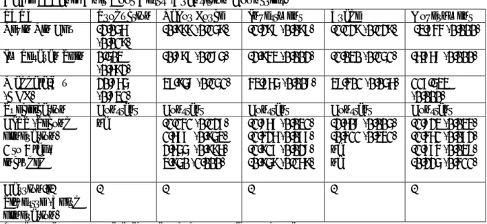
Table 1: Panel Unit Root Tests (EU-Core Countries)
PURT Production Labor Force Investment Trade Government
Levin Lin Chu 0.341 (0.633) -0.967 (0.167) -1.361 (0.087) -0.907 (0.182) 1.055 (0.854) Im Pesaran Shin 0.882 (0.811) 1.016 (0.845) -6.453 (0.000) 0.016 (0.507) -0.038 (0.485) Maddala-Wu (ADF) 30.575 (0.437) 31.614 (0.386) 125.495 (0.000) 26.366 (0.656) 33.980 (0.282)
Specification Constant and Trend
Constant Constant Constant Constant
CIPS (Second generation) 1 to 4 lags included 0.062 (0.525) 0.757 (0.775) 2.340 (0.990) 1.837 (0.967) -1.278 (0.101) 0.268 (0.606) 0.476 (0.683 ) 1.661 (0.048) -2.141 (0.016) 0.086 (0.534) 0.294 (0.616) 1.131 (0.871) 0.514 (0.696) 1.069 (0.857) 2.267 (0.988) 1.124 (0.870) 0.497 (0.690) 1.164 (0.878) 2.267 (0.988) 2.645 (0.996) Carrion-i-Silvestre (Third generation) - - 6.138 (0.000) 5.845 (0.000) - -
Remarks: AIC selection is used to perform first panel generation tests. Carrion-i-Silvestre’s test assumes as the null hypothesis stationarity; it is performed considering a maximum of two structural breaks.
Table 2: Cross-Section Dependence Tests (EU-Core and Transition Countries)
Variable CD test p-Value Correlation Absolute
Correlation Production 33.98 0.00 0.487 0.553 Investment 32.47 0.00 0.470 0.474 Gov Consumption 42.74 0.00 0.617 0.626 Trade 39.60 0.00 0.566 0.591 Labor 59.15 0.00 0.843 0.843
Variable CD test p-Value Correlation Absolute
Correlation Production 26.94 0.00 0.815 0.815 Investment 17.04 0.00 0.532 0.556 Gov Consumption 9.58 0.00 0.302 0.330 Trade 7.21 0.00 0.232 0.367 Labor 11.21 0.00 0.352 0.510
Remarks: The Pesaran (2004) CD test is distributed as a standard normal under the null hypothesis of no cross-sectional dependence and based on mean pair-wise correlation coefficients. It is valid for N and T going to infinity in any order and it is robust to possible structural breaks.
Concerning the EU-core countries (Table 1) and the first generation tests, we do find an integration of order 1 for labor force, trade openness, government consumption, and by construction, the trend. The inflation rate is stationary and will thus be added to the set of exogenous explanatory variables that are outside the cointegration vector. However, the case of investment leads to mixed results since only the LLC test shows no rejection of the null hypothesis of no unit root. As for the transition countries, the results of the first-generation PURT are in favor of the presence of a unit root in the dynamics of the series except again for investment as well as for the government expenditure variable.
Since we expect some contagion and common factor effects between the countries of each subsample – for instance, the core countries share the same monetary policy in the Euro Zone – we perform absolute values of the pairwise correlations and also the Pesaran (2004)11 cross-section dependence test (CD test). As shown in Table 2, not surprisingly we find evidence of significant cross-section dependence between our series. We thus reinvestigate the previous unit root testing and take into account common factors by using so-called second generation PURT from Pesaran (2007) named CIPS. Indeed, when the cross section independence assumption is not verified, the first-generation tests exhibit large size distortions.
Finally, considering that investment series may contain structural breaks that might lead to biased unit root tests results, we also perform the so-called third generation panelunit root test
11 Moscone and Tosetti (2009) evaluate other tests to assess cross-sectional dependence but none perform better
from Carrion-i-Silvestre et al. (2005) that extends a panel KPSS (or Hadri) specification introducing potential structural breaks.
Results from these tests (see the two last lines in Table 1) suggest that investment may be also considered as a nonstationary variable in core countries. The test from Carrion-i-Silvestre et al. (2005) clearly rejects the null of stationarity and all the CIPS results (except with a one-lag specification) are in favor of the unit root hypothesis. However, results are less clear-cut in the transition countries case and the presence of a cointegration relationship needs to be cautiously concluded.
Table 3: Panel Unit Root Tests (Transition Countries)
PURT Production Labor Force Investment Trade Government
Levin Lin Chu -2.056 (0.019) -0.999 (0.159) -1.298 (0.097) -1.129 (0.129) -3.744 (0.000) Im Pesaran Shin 0.503 (0.692) -0.897 (0.185) -2.943 (0.002) -1.030 (0.151) -6.768 (0.000) Maddala-Wu (ADF) 20.865 (0.831) 37.958 (0.151) 43.865 (0.008) 38.401 (0.056) 117.533 (0.000)
Specification Constant Constant Constant Constant Constant
CIPS (Second generation) 1 to 4 lags included na -1.141 (0.127) 1.677 (0.953) 2.655 (0.996) 3.950 (1.000) -1.867 (0.031) -1.426 (0.077) -1.917 (0.028) -0.959 (0.169) -2.608 (0.005) -0.411 (0.341) na na -1.823 (0.034) -1.461 (0.072) -1.774 (0.038) -0.225 (0.411) Carrion-i-Silvestre (Third generation) - - - - -
Remarks: na refers to not available statistics due to the lack of observations.
Regarding previous PURT tests, it should be reasonable to assume that all the variables exhibit I(1) or near I(1) properties, at least in the case of core countries. We thus assess in the next step the null hypothesis of a non-cointegrating relationship against the alternative of cointegration among these variables by relying on Pedroni’s (1999, 2004) as well as Westerlund’s (2007) panel cointegration techniques. The Pedroni first generation cointegration tests are residual tests extending the Engle and Granger methodology in a panel context. Pedroni introduced some heterogeneity in terms of cointegration vectors and developed some pooled (or panel) tests and also some group-mean (or heterogeneous) tests. The results in Table 4 show that four test statistics out of seven lead to reject the null of no cointegration regarding the core countries but only three in the case of transition countries12.
Considering potential cross-section dependence in the production dynamics, we also perform the Westerlund (2007) test based on an ECM approach and on bootstrap critical values robust to the presence of cross-section dependence. Results from the Westerlund test are clearly not in favor of cointegration. However, as the correlation is weak in the case of core countries –
12 Using a simulation study with T=200 and N superior to 5, Orsal (2009) find that the panel-t test has the best
size and size adjusted power properties. On the contrary, the group-p, panel-p and group-t tests have poor size-adjusted powers. Other studies show that Pedroni’s parametric tests perform best in terms of power.
the dependent variable (production) exhibits a correlation value inferior to 0.6 (see Hlouskova and Wagner (2006) and Table 2) - the cross-section dependence issue is of minor importance and we can thus follow the conclusions from Pedroni and argue in favor of a cointegration relationship in both sub-samples.
Note that there were no indications of major breaks in the production dynamics over the period 1995-2010; therefore there was no need to apply cointegration tests that account for structural breaks.
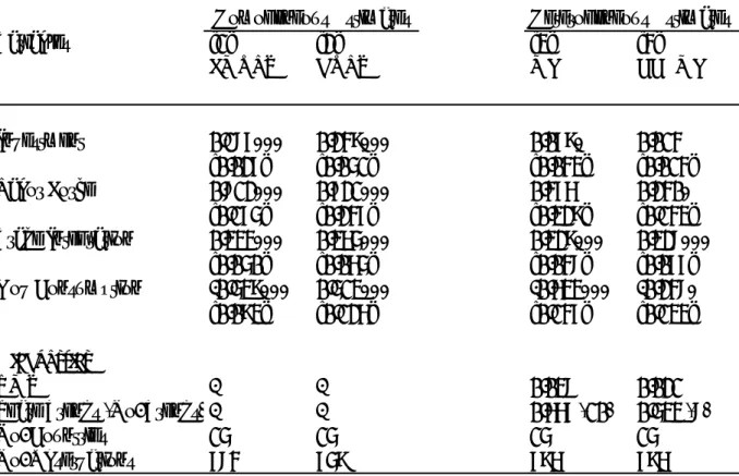
Table 4: Cointegration Tests
EU-Core Countries Transition Countries
Dimension Statistic Standardized
values (p-value) Statistic
Standardized values (p-value) Panel (Pooled) , vN T Z -0.2807 (0.6105) ZvN T, -0.4804 (0.6845) 1 , N T Zρ − -2.5776 (0.0050) ZρN T, −1 -0.5704 (0.2842) , tN T Z -3.809 (0.0000) ZtN T, -2.0309 (0.0211) * , tN T Z 1.4145 (0.9214) ZtN T*, -1.9783 (0.0239) Group (Heterogeneous) !Z ρN ,T−1 -2.3062 (0.0106) !ZρN ,T−1 0.8409 (0.7998) !ZtN ,T -3.9000 (0.0000) !ZtN ,T -1.9512 (0.0255) !ZtN ,T* 1.6485 (0.9504) !ZtN ,T* -1.0817 (0.3107) Westerlund ECM test 1.204 0.51 0.785 0.52 2.128 0.56 2.408 0.84 1.990 0 .77 0.536 0.51 2.024 0.82 1.002 0.63
Remarks: The seven statistics follow a N(0,1) under the null of no cointegration of the Pedroni (1999, 2004) tests. Specification with only a constant but no trend. Z-values and robust p-values with one lag are presented concerning the Westerlund (2007) test. Results with zero or two lags are similar in a qualitative manner.
5.2. Linear Long-Run Estimations
The above cointegration tests have confirmed that a long-run equilibrium relationship between the variables of interest seems to exist. Thus, although the results for the transition countries are not totally clear-cut, we initially employ the Fully Modified Least Squares (FMOLS) estimator, suggested by Pedroni (2000) that allows to profit from the non-stationarity and that corrects the regular pooled OLS estimator for cointegration between the different series and for endogeneity among covariates.
Although the series length should be long enough to avoid small sample bias13, we also estimate with Dynamic Ordinary Least Squares (DOLS), which shows slightly better finite-T handling in the presence of endogenous feedback (Kao and Chiang, 2000) and outperforms the previous FMOLS estimator. The DOLS estimator uses parametric adjustment to the errors by including leads and lags of the differenced I(1) regressors. It is obtained from the following equation:
𝑦!,! = 𝛼! + 𝛽!𝑇!+ 𝛽!𝑋′!,!+ !!!! 𝑐!"∆𝑋!,!!!+ 𝜖!,!
!!!!! , (2) where 𝑐!" is the coefficient of lead or lag values of the differenced explanatory variables 𝑋!,!
including Investment, Labor Force, Trade Integration and Government Consumption variables and 𝑇! represents a time trend. Inflation enters the regression as a deterministic regressor due to not being integrated. Leads and lags are based on the AIC criterion.
Considering the results of the previous cointegration tests in the spirit of Eberhardt and Presbitero (2015), we also employ more flexible estimators, specifically the MG estimator, which accounts for slope heterogeneity, and in light of positive cross-sectional correlation findings, the CCEMG and AMG estimators that allow for both characteristics. The general equation (1) will thus be denoted in the following form:
𝑦!,! = 𝛼!+ 𝛽!𝑇!+ 𝛽!𝑋′!,!+ 𝜖!,!, (3) where cross-sectional dependence arises from a multifactor error structure
𝜖!,! = 𝛼!,!+ 𝜆!𝑓!+ 𝑢!,! (4)
𝑋′!,! = 𝛼!,! + 𝜆!𝑓!+ 𝛾!𝑔!+ 𝜀!,! (5)
Above representation assumes that both the covariates and the error term contain a finite number of unobserved common factors ft, whose impact may differ across countries due to
heterogeneous factor loadings 𝜆!14. The factors ft and gt are allowed to be nonstationary and do
not necessarily remain linear over time. 𝑢!,! and 𝜀!,! are stochastic shocks. The estimators thus accommodate a limited number of strong factors representing global shocks, such as the recent global financial crisis, and an infinite number of weak factors, such as regional spillover effects due to cultural or geographic proximity (Chudik et al., 2011).
The standard MG estimator by Pesaran and Smith (1995) cannot explicitly consider cross-sectional dependence and either assumes the unobservables 𝜆! ft away or tries to catch them
13 Both EU core and transition countries have at least a sample length of 63 periods with a total of 486 panel
observations.
14 g
with a linear trend15. The estimated coefficients 𝛽! are then averaged across countries in the sample.
In order to account for these unobserved common factors in the estimation process, the CCEMG estimator adds as covariates to the regression a linear combination of cross-sectional panel averages of both the dependent and the independent variables (𝑦!, 𝑿!)16. These extra
regressors, however, cannot be interpreted in a meaningful way, but help to consistently estimate the model parameters in the presence of unobserved common factors. Pesaran (2006) demonstrates that the estimator has good finite sample properties and that it is able to control for serially and spatially correlated error terms. Moreover, various simulation studies (e.g. Coakley et al., 2006; Kapetanios et al., 2011) have shown that the CCEMG estimator also performs quite well in presence of non-stationary and cointegrated covariates, global and regional spillover and business cycle effects, as well as structural breaks (Eberhardt and Teal, 2013a, 2013b)17.
Regarding the AMG estimator, it provides a viable alternative to the CCEMG estimator, particularly in the context of cross-country production functions (Bond and Eberhardt, 2013). Whereas in the CCEMG estimator the unobserved common factors have been treated as nuisance, the AMG estimator introduces a “common dynamic process” in the group specific regression. This common dynamic process variable is constructed by taking the coefficients of the t-1 time dummies in a first stage OLS regression run in first differences. In the second step, the group-specific regression model is then augmented with these coefficients along with linear time trends to catch omitted idiosyncratic processes. We resort to including the common dynamic effect as an explicit variable rather than imposing it on each group member by subtracting the process from the dependent variable with a unit coefficient. Like in the MG and the CCEMG estimators, the group-specific model parameters enter the final regression as an average across panel members18 (Eberhardt, 2012). Note, however, that the estimation via AMG serves as robustness check to the CCEMG only, as due to shorter time series for the transition country, subsample estimations with AMG could be only performed for the EU core countries. Results can be found in the Appendix A1.
Table 5 and 6 below present the estimation results on the long-run economic growth relationships for the EU-core and transition subsamples computed with previously described estimators. Whereas estimates of FMOLS and DOLS in columns [1] and [2] imposing
15 Not explicitly controlling for cross-sectional correlation, the MG estimator can thus be considered as a fully
heterogenous estimator.
16 For an accessible study of heterogeneous parameter estimators containing unobserved common factors
consult, for example, Eberhardt et al. (2013).
17 In the presence of common factors, Bai et al. (2009) advocate the updated and fully modified bias corrected
estimators. Recent contributions by Bailey et al. (2012) and Westerlund and Urbain (2015) mark a preference for the CCEMG estimator on the basis of theoretical and computational easiness.
18 Like in the MG and the CCEMG estimators, the group-specific model parameters are averaged across the
panel, i.e. 𝛽!"#=!
! 𝛽! !
!!! . For all MG estimators we follow standard practice in the literature and regress the
parameter homogeneity across countries, the other two models in columns [3] and [4] allow for differential relationships.
Heterogeneous Estimates
[1] [2] [3] [4]
FMOLS DOLS MG CCEMG
Investment 0.187*** 0.249*** 0.079* 0.014 [0.027] [0.051] [0.043] [0.014] Labor Force 0.812*** 0.721*** 0.476 0.240* [0.175] [0.247] [0.329] [0.143] Trade Integration 0.334*** 0.365*** 0.329*** 0.328*** [0.050] [0.065] [0.048] [0.077] Gov Consumption -0.539*** 0.513*** -0.634*** -0.248* [0.093] [0.126] [0.147] [0.133] Diagnostics RMSE - - 0.038 0.021
Share Trends (No. Trends) - - 0.667 (10) 0.533 (8)
No. Countries 15 15 15 15
784 759 796 796
No. Observations
Table 5: Long-Run Determinants of Economic Growth (EU-Core Countries)
Variables
Homogeneous Estimates
Remarks: Estimations are based on FMOLS, DOLS, MG, and CCEMG estimators. Sample: EU core countries, quarterly data from 1995Q1 - 2010Q4. We report the cross-country mean of coefficients in the heterogeneous parameter models [3]-[4] according to Hamilton (1992); standard errors in brackets are non-parametrically constructed following Pesaran and Smith (1995). An intercept, a group-specific linear trend and the quarterly average of the inflation rate as an exogenous variable are included in all models, yet not reported (available upon request). RMSE is the root mean square error; Share Trends (No. Trends) reports the share (number) of group-specific trends significant at the 5% level. *, **, *** indicates significance at the 1%, 5%, or 10% level.
Heterogeneous Estimates
[1] [2] [3] [4]
FMOLS DOLS MG CCEMG
Investment 0.220*** 0.392*** 0.161*** 0.044 [0.022] [0.033] [0.048] [0.028] Labor Force 0.322** 0.233* 0.314 0.19 [0.140] [0.129] [0.313] [0.137] Trade Integration 0.024*** 0.012 0.243*** 0.046 [0.008] [0.008] [0.048] [0.067] Gov Consumption -0.269*** -0.098 -0.072 -0.172* [0.061] [0.081] [0.119] [0.096] Diagnostics RMSE - - 0.044 0.031
Share Trends (No. Trends) - - 1.000 (11) 0.545 (6)
No. Countries 11 11 11 11
502 486 518 518
No. Observations
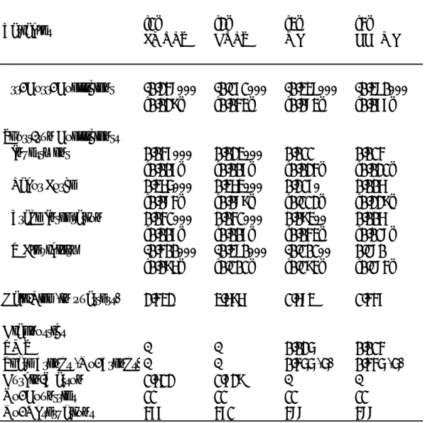
Table 6: Long-Run Determinants of Economic Growth (Transition Countries)
Variables
Homogeneous Estimates
Remarks: Estimations are based on FMOLS, DOLS, MG, and CCEMG estimators. Sample: 11 transition countries, quarterly data from 1995Q1 - 2010Q4. We report the cross-country mean of coefficients in the heterogeneous parameter models [3]-[4] according to Hamilton (1992); standard errors in brackets are non-parametrically constructed following Pesaran and Smith (1995). An intercept, a group-specific linear trend and the quarterly average of the inflation rate as an exogenous variable are included in all models, yet not reported (available upon request). RMSE is the root mean square error; Share Trends (No. Trends) reports the share (number) of group-specific trends significant at the 5% level. *, **, *** indicates significance at the 1%, 5%, or 10% level.
Regression output in both tables exhibits for all coefficients of the employed explanatory variables, according to theory, the expected signs and to a large extent significance19. By closer examining estimation results for EU core countries in Table 5, investment is shown to have a positive impact on long-run economic output, and is, with the exception of the CCEMG estimator, always significant. This is consistent with early results on growth determinants by Barro (1991) and Barro and Lee (1994). Along the lines of standard growth literature, the size of the labor force attracts the largest coefficients among all variables included. The positive and across all specifications pretty stable and highly significant coefficient of the trade integration variable is particularly for core members of the European Union not really surprising. The tight integration in trade of goods and services has since the early set-up of the European Economic Community fostered exports within the EU and has thus tremendously contributed to overall economic growth. The coefficient associated with government consumption is negative and even though more than halved under CCEMG, indicates a
19 This also holds for the AMG estimations of the EU-core subsample in Appendix 1, where the signs of
coefficients also fulfil expectations. However, only trade integration and the common dynamic process remains highly significant.
significant negative relationship between government expenditure and economic output (Fajnzylber et al., 2005; Loayza and Rancière, 2006; Lopez-Villavicencio and Mignon, 2011). High government expenditure can be considered a burden and may over time diminish a government’s “fiscal space”, for instance through having precommitted future budgetary resources to social insurance programs20 (Heller, 2005).
Comparing the results between the EU-core countries and their transition counterparts, we find in Table 6 a stronger contribution of investment to economic output in the transition countries regression. This result echoes the basic theory of decreasing marginal productivity in the growth literature, finding an ever-decreasing marginal impact of any extra unit of capital with respect to advancing economic development (Barro and Sala-i-Martin 2000). Hence, it represents the different levels of economic development in the country subsamples. Whereas the level of capital accumulation is apparently of higher importance for transition countries, labor force size seems to matter on average less for long-term economic output, whose impact is diminished by almost two thirds in the homogeneous estimates and also got diminished under the heterogenous estimators. These results follow two out of the seven stylized transition facts recorded by Campos and Coricelli (2002): that “labor moved”, not geographically but from activity to unemployment, inactivity, and from public to private sector, restoring its contribution to GDP growth, and that investment shrank, from a situation where it was abundant but completely inefficient. The reduction in significance and size of the trade openness variable compared to the EU core may point to some limitations in the unequivocal view of overall beneficent trade openness. Recent literature, for instance, finds a negative effect of export concentration, most likely the case for our transition countries (Lederer and Maloney, 2003). Others stress the importance of policy complementation in non-trade areas with regard to non-trade liberalization, particularly in emerging countries (Chang et al. 2009). For what regards transition countries, the trade collapse was caused by the dismantling of the Council for Mutual Economic Assistance (CMEA) and trade re-orientation. Trade is considered as the main factor, driving the initial huge output losses, and strong subsequent recoveries. Regarding government consumption, although with negative coefficient and significant at least in the FMOLS and to a lesser extent in the CCEMG specification, it seems to be less an issue for transition countries, probably driven by comparably lower Debt-to-GDP levels (Boone and Maurel, 1999).
5.3. Panel Cointegration Framework
As Engle and Granger (1987) pointed out in their seminal work, cointegration and error correction are mirror images of each other. We thus continue by estimating a standard linear Panel Error-Correction Model (Panel ECM) in order to inspect the different convergence forces working on economic growth in either the EU core or transition countries.
20 Defined according to Heller (2005) as “room in a government´s budget that allows it to provide resources for a
desired purpose without jeopardizing the sustainability of its financial position or the stability of the economy”.
Our equations include as short-run fundamentals the previously used variables in first differences and the Kocenda et al. (2013) exchange rate flexibility measure computed as the mean of percent exchange rate changes vis-à-vis the anchor currency Deutsch Mark/Euro. Government consumption as a short-run variable has been discarded21. The subsequent
equation has the following form:
Δ𝑦!,! = 𝜇!+ θ𝑧!,!!!+ 𝛽Δ𝑋′!,!+ 𝜀!,!, (6)
where 𝑧!,!!! represents the respective residuals of the previous long-run growth regressions lagged by one period. What we are most interested in is the respective coefficient 𝜃 that describes in a linear way the adjustment speed to the long-term equilibrium growth rate. ∆𝑋!,! is the vector of short-run controls with ∆ indicating the time series operator for a transformation into growth rates; 𝜀!,! is the i.i.d. residual term of the short-run equation. In addition, to check the robustness of our results and considering the mixed evidence in favor of cointegration – especially in the case of transition countries – and also the potential presence of common factors in the dynamics of the series, we further compute above regression with MG, CCEMG and AMG estimators. Every time the residuals from the respective long-run growth models in the first step are included as error-correction terms. Tables 7 and 8 below show for both country subsamples error-correction coefficients as residuals derived from above estimations in the first step.
21 All estimations have also been performed including the government consumption variable. However, apart
from not being significant, results have shown to be more robust when excluding it from the variable set. Moreover, the insignificance of government consumption as a short-term control also corroborates recent findings of Eberhardt and Presbitero (2015). Results are available upon request.
[1] [2] [3] [4]
FMOLS DOLS MG CCEMG
Err. Corr. Coefficient -0.154*** -0.143*** -0.282*** -0.415***
[0.023] [0.027] [0.043] [0.069] Short-run Coefficients ΔInvestment 0.047*** 0.037*** 0.001 -0.002 [0.007] [0.007] [0.014] [0.011] ΔLabor Force 0.126 0.077 -0.005 0.170 [0.082] [0.083] [0.116] [0.199] ΔTrade Integration 0.275*** 0.259*** 0.268*** 0.043 [0.024] [0.025] [0.063] [0.032] ER Flexibility -0.178 -0.198* -0.037 -0.065 [0.108] [0.111] [0.090] [0.148]
Half-Life (in quarters) 4.145 4.492 2.096 1.295
Diagnostics
RMSE - - 0.022 0.015
Share Trends (No. Trends) - - 0.214 (3) 0.071 (1)
Durbin-Watson 1.995 2.022 -
-No. Countries 15 15 15 15
725 715 780 780
Table 7: Linear Panel Error-Correction Model (EU-Core Countries) Variables
No. Observations
Remarks: FMOLS and DOLS estimations are based on Panel OLS; all specifications contain the respective long-run residuals as error-correction terms. Sample: EU-core countries, quarterly data from 1995Q1 - 2010Q4. We report the cross-country mean of coefficients in the heterogeneous parameter models [3]-[4] according to Hamilton (1992); standard errors in brackets are non-parametrically constructed following Pesaran and Smith (1995). An intercept, a group-specific linear trend and the quarterly average of the inflation rate as an exogenous variable are included in all models, yet not reported (available upon request). RMSE is the root mean square error; Share Trends (No. Trends) reports the share (number) of group-specific trends significant at the 5% level. *, **, *** indicates significance at the 1%, 5%, or 10% level.
[1] [2] [3] [4]
FMOLS DOLS MG CCEMG
Err. Corr. Coefficient -0.248*** -0.171*** -0.338*** -0.380***
[0.029] [0.043] [0.083] [0.077] Short-run Coefficients ΔInvestment 0.047*** 0.023*** 0.011 0.014 [0.007] [0.007] [0.024] [0.021] ΔLabor Force 0.365*** 0.363*** 0.217* 0.006 [0.084] [0.089] [0.112] [0.229] ΔTrade Integration 0.041*** 0.041*** 0.093** 0.006 [0.007] [0.007] [0.043] [0.018] ER Flexibility -0.400*** -0.380*** -0.101** 0.180 [0.096] [0.101] [0.194] [0.184]
Half-Life (in quarters) 2.432 3.696 1.683 1.447
Diagnostics
RMSE - - 0.025 0.014
Share Trends (No. Trends) - - 0.455 (5) 0.445 (5)
Durbin-Watson 1.612 1.729 -
-No. Countries 11 11 11 11
477 471 488 488
Table 8: Linear Panel Error-Correction Model (Transition Countries) Variables
No. Observations
Remarks: FMOLS and DOLS estimations are based on Panel OLS; all specifications contain the respective long-run residuals as error-correction terms. Sample: 11 transition countries, quarterly data from 1995Q1 - 2010Q4. We report the cross-country mean of coefficients in the heterogeneous parameter models [3]-[4] according to Hamilton (1992); standard errors in brackets are non-parametrically constructed following Pesaran and Smith (1995). An intercept, a group-specific linear trend and the quarterly average of the inflation rate as an exogenous variable are included in all models, yet not reported (available upon request). RMSE is the root mean square error; Share Trends (No. Trends) reports the share (number) of group-specific trends significant at the 5% level. *, **, *** indicates significance at the 1%, 5%, or 10% level.
Across all models in Tables 7 and 8, there is strong evidence of error correction as the high significance and the negative sign of the error-correction terms show. Of strong interest is the difference in speed of adjustment to the long-term growth equilibrium, to which the transition country group seems to converge faster than EU core countries under the two homogeneous and the heterogenous estimators in columns [1] – [4], both not accounting and accounting for cross-sectional dependence22. Consequently, whereas the developed EU economies show
highly significant error-correction coefficients of between -0.154 with FMOLS and -0.415 under CCEMG, transition countries report coefficients of -0.248 and -0.380 respectively. As an additional indication of convergence speed, we also compute the half-life23 (here measured in quarters), which indicates “the length of time after a shock before the deviation in output shrinks to half of its impact” (Chari et al., 2000, p. 1161). In line with in size decreasing error-correction coefficients, the half-life values decline from about 4.5 to 1.3 quarters for the EU-core and from 3.7 to 1.4 for the transition countries according to the different model specifications. Even though error-correction coefficients show an increasing and half-life respectively a decreasing trend for both country groups with a continuous refinement of the estimator, values constantly remain higher throughout all estimators for the transition subsample. The overall tendency thus seems to confirm a somewhat faster adjustment of transition economies.
A quick look at the short run controls for both country groups reveals, where significant, a positive relation with long-run growth across all specifications, except for exchange rate flexibility. The size of the investment coefficients does not vary considerably between EU-core and transition countries, and attracts a strong significance under the homogenous FMOLS and DOLS estimators. This result is not confirmed by the heterogeneous MG and CCEMG estimators, albeit with slightly higher investment coefficients for transition countries. Moreover, the size of the labor force seems to play a greater role as emphasized by larger coefficients and higher significance for the transition country sample. Conversely, trade integration matters more for the EU-core than for growth in emerging Europe; if significant, coefficients are again higher, what is in line with growth theory and previously pointed out structural reasons. This result may thus again reflect the close and long-lasting interconnectedness of Western European economies, while European integration is still fragmented and ongoing for Eastern Europe. As for exchange rate flexibility, the opposite is true as apparently higher flexibility in the short run implies lower long-term growth for transition countries. The latter findings contrast somewhat with Kocenda et al. (2013) who find mildly positive short-run effects of exchange rate flexibility, though a negative impact over the longer term.
Note that the declining significance of many short-term controls under the heterogenous estimators does not imply an absence of any significant effects, but rather emphasizes the heterogeneity across countries with dynamics on average cancelling out.
The analysis up to this point investigated long-term behavior of economic growth and the speed of convergence for the two different subsamples, EU-core and transition countries. A number of empirical models were assessed and we can conclude that error-correction is taking place. Results further depict a faster return of transition countries to their long-term growth. To explore nonlinearity of convergence, we now turn to an empirical model class that allows for different regimes in the process by relying on endogenous thresholds and by modeling a smooth process of potential regime-switches that are dependent on transition variables.
6. Nonlinear Specification
Results from the previous section suggest that convergence among countries towards their long-run growth trend in the two different country groups is not homogenous, but may rather depend on other specific factors, such as the controls examined before. We further assume, that the relation between these factors and the speed of convergence may be nonlinear in nature or may contain a nonlinear adjustment mechanism for different country groups and economic fundamentals, a feature the previous linear models would be unable to capture. In order to further disentangle these relationships, we extend the previous linear error-correction framework and employ a panel smooth transition regression model developed by González et al. (2005) and Fok et al. (2005), following the work of Granger and Teräsvirta (1993) in a time series context. Panel smooth transition regression models allow for the modeling of different regimes and inherent nonlinear and time-varying convergence processes across countries and over time. In this particular model specification, the transition from one regime to the other is smooth and not discrete, as in the predecessor models of panel threshold regressions (PTR) developed by Hansen (1999).
6.1. Methodology
In general, the approach follows the three-step strategy by González et al. (2005) for PSTR models: (i) identification, (ii) estimation, and (iii) evaluation. In the identification step, homogeneity is tested against the nonlinear PSTR alternative and upon confirmation of non-linearity, a transition function either specified as m = 1 (logistic) or m = 2 (exponential) is to be selected24. The second step involves estimation of the model by multivariate non-linear least squares (NLS) once the data have been demeaned. In the evaluation step validity of the estimated model is verified along with a determination of the number of regimes, i.e. testing for non-remaining linearity.
First, the linear specification of our growth equation is tested against a PSTR alternative with threshold effects. We do so by testing the null hypothesis 𝛾 = 0. Due to the presence of unidentified nuisance parameters under the null, the transition function 𝑔(𝑠!,!!!; 𝛾, 𝑐) is replaced by its first-order Taylor expansion around zero, following Luukonen et al. (1988) and González et al. (2005).
Two tests are usually identified in the literature to test for the linearity hypothesis 𝛾 = 0, or equivalently 𝛽!∗ = ⋯ = 𝛽
!∗ = 0, namely the LM, the pseudo LRT, and the LMF statistics25.
Since Van Dijk et al. (2002) report better size properties in small samples for the F-statistic than the 𝜒! based statistic, we only base our judgement on the F-statistic.
24 From an empirical point of view, González et al. (2005) mention that only cases of m =1 and m = 2 suffice to
capture nonlinearities due to regime switching.
25 The LM and pseudo-LRT statistics have a 𝜒! distribution with mK degrees of freedom; the F statistic has a