Tropospheric ozone changes, radiative forcing and attribution to emissions in the Atmospheric Chemistry and Climate Model Intercomparison Project (ACCMIP)

HAL Id: hal-03048310

https://hal.archives-ouvertes.fr/hal-03048310

Submitted on 10 Dec 2020

HAL is a multi-disciplinary open access

archive for the deposit and dissemination of

sci-entific research documents, whether they are

pub-lished or not. The documents may come from

teaching and research institutions in France or

abroad, or from public or private research centers.

L’archive ouverte pluridisciplinaire HAL, est

destinée au dépôt et à la diffusion de documents

scientifiques de niveau recherche, publiés ou non,

émanant des établissements d’enseignement et de

recherche français ou étrangers, des laboratoires

publics ou privés.

attribution to emissions in the Atmospheric Chemistry

and Climate Model Intercomparison Project (ACCMIP)

D. Stevenson, P. Young, V. Naik, J.-F. Lamarque, D. Shindell, A.

Voulgarakis, R. Skeie, S. Dalsoren, G. Myhre, T. Berntsen, et al.

To cite this version:

D. Stevenson, P. Young, V. Naik, J.-F. Lamarque, D. Shindell, et al.. Tropospheric ozone changes,

radiative forcing and attribution to emissions in the Atmospheric Chemistry and Climate Model

Inter-comparison Project (ACCMIP). Atmospheric Chemistry and Physics, European Geosciences Union,

2013, 13 (6), pp.3063-3085. �10.5194/ACP-13-3063-2013�. �hal-03048310�

Atmos. Chem. Phys., 13, 3063–3085, 2013 www.atmos-chem-phys.net/13/3063/2013/ doi:10.5194/acp-13-3063-2013

© Author(s) 2013. CC Attribution 3.0 License.

EGU Journal Logos (RGB)

Advances in

Geosciences

Open Access

Natural Hazards

and Earth System

Sciences

Annales

Geophysicae

Nonlinear Processes

in Geophysics

Atmospheric

Chemistry

and Physics

Atmospheric

Chemistry

and Physics

Atmospheric

Measurement

Techniques

Atmospheric

Measurement

Techniques

Biogeosciences

Open Access Open Access

Biogeosciences

Discussions

Climate

of the Past

Open Access Open Access

Climate

of the Past

Discussions

Earth System

Dynamics

Open Access Open Access

Earth System

Dynamics

Geoscientific

Instrumentation

Methods and

Data Systems

Open Access

_{Geoscientific}

Instrumentation

Methods and

Data Systems

Geoscientific

Model Development

Open Access Open Access

Geoscientific

Model Development

Hydrology and

Earth System

Sciences

Hydrology and

Earth System

Sciences

Ocean Science

Open Access Open Access

Ocean Science

Discussions

Solid Earth

Open Access Open Access

Solid Earth

Open Access Open Access

The Cryosphere

Natural Hazards

and Earth System

Sciences

Open Access

Discussions

Tropospheric ozone changes, radiative forcing and attribution to

emissions in the Atmospheric Chemistry and Climate Model

Intercomparison Project (ACCMIP)

D. S. Stevenson1, P. J. Young2,3,*, V. Naik4, J.-F. Lamarque5, D. T. Shindell6, A. Voulgarakis7, R. B. Skeie8, S. B. Dalsoren8, G. Myhre8, T. K. Berntsen8, G. A. Folberth9, S. T. Rumbold9, W. J. Collins9,**, I. A. MacKenzie1, R. M. Doherty1, G. Zeng10, T. P. C. van Noije11, A. Strunk11, D. Bergmann12, P. Cameron-Smith12, D. A. Plummer13, S. A. Strode14,15, L. Horowitz16, Y. H. Lee6, S. Szopa17, K. Sudo18, T. Nagashima19, B. Josse20, I. Cionni21, M. Righi22, V. Eyring22, A. Conley5, K. W. Bowman23, O. Wild24, and A. Archibald25

1_{School of GeoSciences, The University of Edinburgh, Edinburgh, UK}

2_{Chemical Sciences Division, NOAA Earth System Research Laboratory, Boulder, Colorado, USA}

3_{Cooperative Institute for Research in Environmental Sciences, University of Colorado, Boulder, Colorado, USA} 4_{UCAR/NOAA Geophysical Fluid Dynamics Laboratory, Princeton, New Jersey, USA}

5_{National Center for Atmospheric Research, Boulder, Colorado, USA}

6_{NASA Goddard Institute for Space Studies and Columbia Earth Institute, New York, NY, USA} 7_{Department of Physics, Imperial College London, London, UK}

8_{CICERO, Center for International Climate and Environmental Research-Oslo, Oslo, Norway} 9_{Met Office Hadley Centre, Exeter, UK}

10_{National Institute of Water and Atmospheric Research, Lauder, New Zealand} 11_{Royal Netherlands Meteorological Institute, De Bilt, the Netherlands} 12_{Lawrence Livermore National Laboratory, Livermore, California, USA}

13_{Canadian Centre for Climate Modeling and Analysis, Environment Canada, Victoria, British Columbia, Canada} 14_{NASA Goddard Space Flight Centre, Greenbelt, Maryland, USA}

15_{Universities Space Research Association, Columbia, MD, USA}

16_{NOAA Geophysical Fluid Dynamics Laboratory, Princeton, New Jersey, USA} 17_{Laboratoire des Sciences du Climat et de l’Environment, Gif-sur-Yvette, France}

18_{Department of Earth and Environmental Science, Graduate School of Environmental Studies, Nagoya University, Nagoya,}

Japan

19_{National Institute for Environmental Studies, Tsukuba-shi, Ibaraki, Japan}

20_{GAME/CNRM, M´et´eo-France, CNRS – Centre National de Recherches M´et´eorologiques, Toulouse, France}

21_{Agenzia Nazionale per le Nuove Tecnologie, l’energia e lo Sviluppo Economico Sostenibile (ENEA), Bologna, Italy} 22_{Deutsches Zentrum f¨ur Luft- und Raumfahrt (DLR), Institut f¨ur Physik der Atmosph¨are, Oberpfaffenhofen, Germany} 23_{NASA Jet Propulsion Laboratory, Pasadena, California, USA}

24_{Lancaster Environment Centre, University of Lancaster, Lancaster, UK} 25_{Centre for Atmospheric Science, University of Cambridge, UK}

*_{now at: Lancaster Environment Centre, University of Lancaster, Lancaster, UK} **_{now at: Department of Meteorology, University of Reading, UK}

Correspondence to: D. S. Stevenson (david.s.stevenson@ed.ac.uk)

Received: 31 July 2012 – Published in Atmos. Chem. Phys. Discuss.: 4 October 2012 Revised: 16 February 2013 – Accepted: 21 February 2013 – Published: 15 March 2013

Abstract. Ozone (O3) from 17 atmospheric chemistry

mod-els taking part in the Atmospheric Chemistry and Climate Model Intercomparison Project (ACCMIP) has been used to calculate tropospheric ozone radiative forcings (RFs). All models applied a common set of anthropogenic emissions, which are better constrained for the present-day than the past. Future anthropogenic emissions follow the four Repre-sentative Concentration Pathway (RCP) scenarios, which de-fine a relatively narrow range of possible air pollution emis-sions. We calculate a value for the pre-industrial (1750) to present-day (2010) tropospheric ozone RF of 410 mW m−2. The model range of pre-industrial to present-day changes in O3 produces a spread (±1 standard deviation) in RFs

of ±17 %. Three different radiation schemes were used – we find differences in RFs between schemes (for the same ozone fields) of ±10 %. Applying two different tropopause definitions gives differences in RFs of ±3 %. Given addi-tional (unquantified) uncertainties associated with emissions, climate-chemistry interactions and land-use change, we esti-mate an overall uncertainty of ±30 % for the tropospheric ozone RF. Experiments carried out by a subset of six mod-els attribute tropospheric ozone RF to increased emissions of methane (44±12 %), nitrogen oxides (31 ± 9 %), carbon monoxide (15 ± 3 %) and non-methane volatile organic com-pounds (9 ± 2 %); earlier studies attributed more of the tro-pospheric ozone RF to methane and less to nitrogen oxides. Normalising RFs to changes in tropospheric column ozone, we find a global mean normalised RF of 42 mW m−2DU−1, a value similar to previous work. Using normalised RFs and future tropospheric column ozone projections we calculate future tropospheric ozone RFs (mW m−2; relative to 1750) for the four future scenarios (RCP2.6, RCP4.5, RCP6.0 and RCP8.5) of 350, 420, 370 and 460 (in 2030), and 200, 300, 280 and 600 (in 2100). Models show some coherent re-sponses of ozone to climate change: decreases in the trop-ical lower troposphere, associated with increases in water vapour; and increases in the sub-tropical to mid-latitude up-per troposphere, associated with increases in lightning and stratosphere-to-troposphere transport. Climate change has relatively small impacts on global mean tropospheric ozone RF.

1 Introduction

Ozone (O3)is a radiatively active gas in Earth’s atmosphere, interacting with down-welling and up-welling solar (short-wave, SW) and terrestrial (long(short-wave, LW) radiation. Any changes in the atmospheric distribution of ozone contribute to the radiative forcing of climate change (e.g., Lacis et al., 1990; Forster et al., 2007). The focus of this paper is the tro-posphere, where ozone is thought to have substantially creased since the pre-industrial era, exerting a warming in-fluence on surface climate.

Tropospheric ozone is a secondary pollutant produced dur-ing the photochemical oxidation of methane (CH4), car-bon monoxide (CO) and non-methane volatile organic com-pounds (NMVOC) in the presence of nitrogen oxides (NOx)

(Crutzen, 1974; Derwent et al., 1996). Downwards transport of ozone from the stratosphere is also an important source of tropospheric ozone (Stohl et al., 2003; Hsu and Prather, 2009). Completing its budget, ozone is removed from the troposphere by several chemical reactions (Crutzen, 1974), and is also dry deposited at the surface, mainly to vegetation (Fowler et al., 2009).

Emissions of ozone precursors from anthropogenic and biomass burning sources have changed (generally risen) dra-matically since the pre-industrial era (Lamarque et al., 2010), tending to drive up tropospheric ozone concentrations. In-creasingly sophisticated models of atmospheric chemistry, transport, and surface exchange, driven by emission esti-mates, and sometimes coupled to climate models, have been used to simulate the rise of ozone since industrialisation (Hough and Derwent, 1990; Crutzen and Zimmerman, 1991; Berntsen et al., 1997; Wang and Jacob, 1998; Gauss et al., 2006).

Modelled increases in ozone are, however, difficult to evaluate against observations. Past estimates of many at-mospheric constituents can be derived from analyses of air trapped in bubbles during ice formation (Wolff, 2011), but ozone is too reactive to be preserved in this way. Direct mea-surements of tropospheric ozone concentrations prior to the 1970s are also extremely limited (Volz and Kley, 1988; Stae-helin et al., 1994), and most early measurements used rela-tively crude techniques, such as Sch¨onbein papers (Rubin, 2001), that are subject to contamination from compounds other than ozone (Pavelin et al., 1999). Only in the last few decades have observation networks and analytical methods developed sufficiently to allow a global picture of ozone’s distribution in the troposphere to emerge (Fishman et al., 1990; Logan, 1999; Oltmans et al., 2006; Thouret et al., 2006). Observational data have been used to analyse past trends (e.g., Cooper et al., 2010; Logan et al., 2012; Parrish et al., 2012; Tilmes et al., 2012; Wilson et al., 2012; Oltmans et al., 2013). These studies indicate that: (i) inter-annual vari-ability in ozone, and in some cases changes in observing techniques, make trends difficult to observe; nevertheless, (ii) there is good evidence that Northern Hemisphere mid-latitude ozone increased by ∼ 1 % yr−1 from ∼ 1950–2000 (i.e. roughly doubled); and (iii) this growth has slowed or stopped over the last decade or so, possibly related to emis-sions controls.

Although changes in anthropogenic precursor emissions have probably been the main driver of ozone change, sev-eral other factors may also have contributed. Natural sources of precursor emissions (e.g., wetland CH4, soil and

light-ning NOx, biogenic NMVOCs) show significant

variabil-ity and have probably also changed since the pre-industrial era, but these changes are highly uncertain (e.g., Arneth et

al., 2010). The stratospheric source has probably been af-fected by stratospheric ozone depletion, and is forecast to change in the future, via ozone recovery and acceleration of the Brewer-Dobson circulation (Hegglin and Shepherd, 2009; Zeng et al., 2010; SPARC-CCMVal, 2010), although attempts to diagnose circulation changes from observations have given ambiguous results (Engel et al., 2009; Lin et al., 2009; Ray et al., 2010; Young et al., 2012). Ozone’s removal, via chemical, physical and biological processes is also sub-ject to variability and change. Increases in absolute humid-ity (driven by warming), changes in ozone’s distribution, and changes in hydroxyl (OH) and peroxy (HO2)radicals, have all tended to increase chemical destruction of ozone (John-son et al., 2001; Steven(John-son et al., 2006; Isaksen et al., 2009). Dry deposition of ozone at the surface, and to vegetation in particular, has been influenced by land-use change, but also by changes in climate and CO2abundance (Sanderson

et al., 2007; Sitch et al., 2007; Fowler et al., 2009; Ander-sson and Engardt, 2010; Ganzeveld et al., 2010; Wu et al., 2012). Fluctuations in these natural sources and sinks are driven by climate variability; climate change and land-use change may also have contributed towards long-term trends in ozone (Stevenson et al., 2005).

We use the concept of radiative forcing (RF) to quantify the impacts of tropospheric ozone changes on Earth’s radi-ation budget since the pre-industrial period. Specifically, in this paper we follow the Intergovernmental Panel on Climate Change (IPCC) and use the following definition of RF from their Third Assessment Report (Ramaswamy et al., 2001): “The change in the net (down minus up) irradiance (solar plus longwave; in W m−2)at the tropopause after allowing for stratospheric temperatures to readjust to radiative equi-librium, but with surface and tropospheric temperatures and state held fixed at unperturbed values.”

Previous estimates of the tropospheric ozone RF (e.g., Gauss et al., 2006) span the range 250–650 mW m−2, with a central value of 350 mW m−2for the RF from 1750–2005 (Forster et al., 2007). Skeie et al. (2011) recently estimated a value of 440 mW m−2, with an uncertainty of ±30 %, us-ing one of the models we also use in this study. Cionni et al. (2011) calculated ozone RFs for the IGAC/SPARC (Inter-national Global Atmospheric Chemistry/Stratospheric Pro-cesses and their Role in Climate) ozone database, and found a tropospheric ozone RF (1850s–2000s) of 230 mW m−2, us-ing an earlier version of the main radiation scheme used here. Using an updated version of this radiation scheme with exactly the same ozone fields we find an equivalent, and presumed more accurate, value of 320 mW m−2. The tropospheric part of the IGAC/SPARC ozone database was constructed from early Atmospheric Chemistry and Climate Model Intercomparison Project (ACCMIP) integrations from two of the 17 models used here (GISS-E2-R and NCAR-CAM3.5). Through the use of additional models, we consider the multi-model mean results presented here to be a more

ro-bust estimate of atmospheric composition change than the IGAC/SPARC database.

It is useful to understand how specific emissions of ozone’s precursors have driven up its concentration (e.g., Wild et al., 2012). Model experiments carried out by Shindell et al. (2005, 2009) attributed pre-industrial to present-day ozone changes to increases in CH4, NOx, CO and NMVOC

emissions, finding that methane emissions were responsible for most of the ozone change. These emissions also influ-ence the oxidising capacity of the atmosphere in general, and affect a range of radiatively active species beyond ozone, including methane and secondary aerosols (Shindell et al., 2009).

In this paper, we present results from global models par-ticipating in the ACCMIP (see www.giss.nasa.gov/projects/ accmip). Within ACCMIP, multiple models simulated at-mospheric composition between 1850–2100. Lamarque et al. (2013) give an overview of ACCMIP and present detailed descriptions of the participating models and model simula-tions. Shindell et al. (2012) describe total radiative forcings, particularly those from aerosols; Lee et al. (2012) further fo-cus on black carbon aerosol. Young et al. (2013) describe the ozone results in detail, including a range of comparisons with observations. Fiore et al. (2012) review air quality and cli-mate change, and present future ozone projections from the ACCMIP models. Bowman et al. (2012) focus on compar-isons of modelled ozone with measurements from TES (Tro-pospheric Emission Spectrometer). Voulgarakis et al. (2013) and Naik et al. (2012) document the evolution of the oxidis-ing capacity of the atmosphere, especially OH and its impact on methane lifetime.

This paper looks in detail at tropospheric ozone RFs from the ACCMIP simulations. In Sect. 2, the models used and the experiments they performed are described. Results of sim-ulated ozone and resulting radiative forcings are presented in Sect. 3; these are discussed and conclusions are drawn in Sect. 4. For conciseness, the main text focusses on gener-alised results (often presented as the multi-model mean) and specific results from individual models are predominantly presented in the Supplement.

2 Methods

2.1 Models employed

Results from 17 different models are analysed here (Table 1). Detailed model descriptions are provided in Lamarque et al. (2013); for model Q (TM5) see: Huijnen et al. (2010) and Von Hardenberg et al. (2012). All are global atmospheric chemistry models, and most are coupled to climate mod-els, which provide the driving meteorological fields. Climate model output of sea-surface temperatures and sea-ice con-centrations (SST/SIC) from prior CMIP5 runs typically pro-vide the lower boundary conditions; well-mixed atmospheric

Table 1. Models and experiment run lengths (in years). All models ran with emissions for the 1850s and 2000s; the years specified correspond to the years specified for the climate (SST/SIC).

Experiments (as used in this paper)

Model 1850sa 2000sb Attribc 1Climd Futuree A. CESM-CAM-superfast 10 10 – 10 YnYY B. CICERO-OsloCTM2 1 (2006) 1 (2006) 1 – YYnY C. CMAM 10 10 – – nYnY D. EMAC 10 10 – – nYnY E. GEOSCCM 10 (1870s) 14 (1996–) – – nnnn F. GFDL-AM3 10 (1860s) 10 – 10 YYYY G. GISS-E2-Rf 10 (×5) 10 (×5) – 40 YYYY H. GISS-E2-R-TOMAS 10 10 – 10 nnnn I. HadGEM2 10 (1860s) 10 – 10 YYnY J. HadGEM2-ExtTC 10 (2000s) 10 10 – nnnn K. LMDzORINCA 10 5 (1996–) – – YYYY L. MIROC-CHEM 11 (1850–) 11 (2000–) – 5 (1850–) YnYY M. MOCAGE 4 (1850–) 4 (2000–) – 4 (1850–) YnYY N. NCAR-CAM3.5 8 (1852–) 8 (2002–) 8 8 (1852–) YYYY O. STOC-HadAM3 10 10 10 10 YnnY P. UM-CAM 10 10 (1996–) 10 10 YYnY Q. TM5 1 (2006) 1 (2006) 1 – nnnn a_{Where models did not run 1850–1859 or 1851–1860, the climate model decade ran is indicated. Where other than 10} yr were ran, the starting year is shown.

b_{Where models did not run 2000–2009 or 2001–2010, the climate model years ran are indicated. Where other than 10} yr were ran, the starting year is shown.

c_{Details of the attribution experiments are given in Sect. 3.1.2.} d_{Details of the climate experiments are given in Sect. 3.3.}

e_{The code shown corresponds to the four future scenarios (RCP2.6, RCP4.5, RCP6.0 and RCP8.0, in order). “Y“} indicates that the scenario was run, “n“ indicates that it was not.

f_{Model G ran five ensembles of the 1850s and 2000s experiments, and an average of the five ensembles is used.}

greenhouse gas concentrations are also specified. Three mod-els (B, Q and M) are chemistry-transport modmod-els, driven by offline meteorological analyses (B and Q) or offline output from a climate model (M). Additionally, models B and Q provide only a single year’s output for each experiment and were run with the same meteorology in each case. In all other models, the chemistry module is embedded within a general circulation model. With the exception of models O and P, the calculated chemical fields are used in the climate model’s ra-diation scheme; i.e. they are fully coupled chemistry-climate models (CCM). Models G and H are two versions of GISS-E2-R, but set up in different ways: G has a fully interac-tive coupled ocean (the only model with this) whilst H uses SST/SIC from GISS-E2-R but also includes a more sophis-ticated aerosol microphysics scheme instead of the simpler mass-based scheme used in G. Models I and J are two ver-sions of HadGEM2: I uses a relatively simple tropospheric chemistry scheme, whereas J has a more detailed scheme with several hydrocarbons. Several models (C, D, E, F, G, H, L, M, and N) include detailed stratospheric chemistry schemes; tropospheric schemes range from simple methane oxidation (C) through models with a basic representation of NMVOCs (A, G, H, I, and P) to those with more detailed hy-drocarbon schemes (B, D, E, F, J, K, L, M, N, O and Q). In

addition, some models include interactions between aerosols and gas-phase chemistry (B, F, G, H, I, J, K, L, N, and Q).

Models without detailed stratospheric chemistry handled their upper levels in a variety of different ways. Model A sim-ulated stratospheric ozone using the LINOZ scheme (McLin-den et al., 2000). Model B used monthly model climato-logical values of ozone and nitrogen species, except in the three lowermost layers of the stratosphere (approximately 2.5 km) where the tropospheric chemistry scheme is applied to account for photochemical ozone production (Skeie et al., 2011). Models I, J, K, O, P and Q all used the IGAC/SPARC ozone database (Cionni et al., 2011) to prescribe ozone in the stratosphere. In models I and J, ozone is overwritten in all model levels which are 3 levels (approximately 3–4 km) above the tropopause. Model O used the ozone fields to-gether with vertical winds, to calculate a vertical ozone flux at 100 hPa, added as an ozone source at these levels in regions of descent. Model P prescribed ozone at pressures below 100 hPa between 50◦S–50◦N and pressures below 150 hPa poleward of 50◦, and model Q at pressures below 45 hPa be-tween 30◦S–30◦N and pressures below 90 hPa poleward of 30◦.

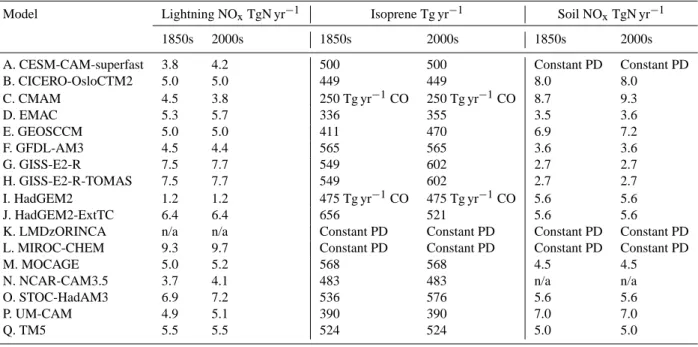
Some models allowed natural emissions of ozone precur-sors to vary with climate; others fixed these sources (Table 2).

Table 2. Natural emissions (lightning NOx, biogenic isoprene, soil NOx) in 1850s and 2000s. Two models (C and I) that did not include isoprene in their chemical schemes included surrogate emissions of CO. Some values are not available (n/a); where values are not available, but models ran with constant present-day (PD) values, this is indicated.

Model Lightning NOxTgN yr−1 Isoprene Tg yr−1 Soil NOxTgN yr−1 1850s 2000s 1850s 2000s 1850s 2000s A. CESM-CAM-superfast 3.8 4.2 500 500 Constant PD Constant PD B. CICERO-OsloCTM2 5.0 5.0 449 449 8.0 8.0 C. CMAM 4.5 3.8 250 Tg yr−1CO 250 Tg yr−1CO 8.7 9.3 D. EMAC 5.3 5.7 336 355 3.5 3.6 E. GEOSCCM 5.0 5.0 411 470 6.9 7.2 F. GFDL-AM3 4.5 4.4 565 565 3.6 3.6 G. GISS-E2-R 7.5 7.7 549 602 2.7 2.7 H. GISS-E2-R-TOMAS 7.5 7.7 549 602 2.7 2.7 I. HadGEM2 1.2 1.2 475 Tg yr−1CO 475 Tg yr−1CO 5.6 5.6 J. HadGEM2-ExtTC 6.4 6.4 656 521 5.6 5.6

K. LMDzORINCA n/a n/a Constant PD Constant PD Constant PD Constant PD L. MIROC-CHEM 9.3 9.7 Constant PD Constant PD Constant PD Constant PD

M. MOCAGE 5.0 5.2 568 568 4.5 4.5

N. NCAR-CAM3.5 3.7 4.1 483 483 n/a n/a

O. STOC-HadAM3 6.9 7.2 536 576 5.6 5.6

P. UM-CAM 4.9 5.1 390 390 7.0 7.0

Q. TM5 5.5 5.5 524 524 5.0 5.0

The models produce a range of results (see below), and each model has its own particular strengths and weaknesses. We know of no major model bugs or gross errors in the simu-lations presented here which might suggest that any of the models should be excluded. We have conducted a partial model evaluation (e.g., Young et al., 2013; Naik et al., 2012), and we can identify some models as outliers, although it is not clear that these outliers are necessarily the models that are most poorly representing the real world. Consequently, in our analysis we retain all models, and produce multi-model means and standard deviations based on all models. Outliers are discussed at various points in the following analysis.

2.2 Model simulations

The main experiments analysed here are multi-annual simu-lations for the 1850s and the 2000s. Every model performed these experiments. Table 1 shows the model run length for each experiment: typically 10 yr, but in a few cases longer or shorter. Model G ran five 10-yr ensemble members. In most cases, models simulated climates of the 1850s and 2000s, typically by specifying SST/SIC fields (typically decadally averaged from prior coupled ocean-atmosphere climate sim-ulations) and setting well-mixed greenhouse gas concentra-tions at appropriate levels. Models B, J and Q ran with the same climate in the 1850s as in their 2000s runs, so only as-sess how emissions have changed composition; single year experiments are thus not unreasonable in these cases.

All models used anthropogenic emissions (including biomass burning emissions, which are partly anthropogenic

and partly natural) from Lamarque et al. (2010). A conse-quence of this approach is that we cannot directly use our results to estimate uncertainties in ozone RF stemming from uncertainties in anthropogenic emissions. On the other hand, this harmonisation of all models to the same source of emis-sions removes a potentially large source of inter-model dif-ference (cf. Gauss et al., 2006). However, as each model did not run exactly the same years to represent the 1850s and 2000s (see Table 1), and models used a range of values for natural emissions (Table 2) there are still some differences between models in the magnitude of the applied change in emissions (see Young et al., 2013, Fig. 1). Note that the model years specified in Table 1 refer to nominal years for the driving climate, but not for the emissions. These differ-ences are added to by different chemistry schemes and deci-sions within each model of how to partition NMVOC emis-sions between individual species and/or to emit directly as CO emissions.

Most models ran with prescribed methane concentrations of around 791 ppbv (1850s) and 1751 ppbv (2000s) (Prinn et al., 2000; Meinshausen et al., 2011). One model (K) ran with methane emissions for the historical period, allow-ing methane concentrations to evolve, although they quite closely follow observations (Szopa et al., 2012).

Six of the models (Table 1) ran a series of attribution ex-periments, based on the 2000s simulations. In these, specific drivers of ozone change (anthropogenic emissions of NOx,

CO, NMVOCs, and CH4concentrations) were individually

reduced to 1850s levels. These experiments are closely re-lated to previous studies with the GISS model (Shindell et

0 10 20 30 40 50 60 70 80 100 150 300 1000 90S 60S 30S 0 30N 60N 90N 1.0 0.9 0.8 0.7 0.6 0.5 0.4 0.3 0.2 0.1 (a) MMM 1850s AZM O3 / ppb

Hybrid vertical level

0 10 20 30 40 50 60 70 80 100 150 300 1000 90S 60S 30S 0 30N 60N 90N 1.0 0.9 0.8 0.7 0.6 0.5 0.4 0.3 0.2 0.1 (c) MMM 2000s AZM O3 / ppb

Hybrid vertical level

-1000 -100 -10 -5 -0.01 0.01 5 10 15 20 25 30 35 40 50 100 90S 60S 30S 0 30N 60N 90N 1.0 0.9 0.8 0.7 0.6 0.5 0.4 0.3 0.2 0.1

(e) MMM 2000s-1850s AZM ∆O3 / ppb

Hybrid vertical level

7 10 13 16 19 22 25 28 31 34 37 40 43 46 49 (b) MMM 1850s ATC O3 (19.8) DU 7 10 13 16 19 22 25 28 31 34 37 40 43 46 49 (d) MMM 2000s ATC O3 (28.1) DU -15 -12.5 -10 -7.5 -5 -2.5 -0.25 0.25 2.5 5 7.5 10 12.5 15 17.5 20 22.5 25 (f) MMM 2000s-1850s ATC ∆O3 (8.4) DU

Fig. 1. Multi-model mean (MMM) annual zonal mean (AZM) ozone (ppb) and annual mean tropospheric column (ATC) ozone (DU), for the: 1850s (a–b), 2000s (c–d) and for the change 2000s–1850s (e–f). The MASKZMT tropopause is used, and area-weighted global mean values of ATC are given in brackets. Figure S1 (Supplement) shows equivalent plots for all individual models.

al., 2005, 2009), and allow us to attribute methane and ozone radiative forcings since the 1850s to these individual drivers, although we do not consider how the individual drivers inter-act.

A subset of ten models (Table 1) ran experiments where they fixed emissions at 2000s levels, but applied an 1850s climate. These simulations allow us to investigate how cli-mate change has contributed to the ozone change since the 1850s. Nine of these models also ran equivalent experiments for future climates.

Finally, most models (Table 1) ran additional historical and future simulations, using harmonized emissions from the Representative Concentration Pathway (RCP) scenarios, and prescribing methane concentrations (Meinshausen et al., 2011). Models K and G ran with methane emissions in the future, allowing methane concentrations to freely evolve. Ozone fields from these experiments are presented in detail by Young et al. (2013) – here we use future tropospheric col-umn ozone changes in conjunction with normalised radiative forcings (mW m−2DU−1) to estimate future tropospheric ozone radiative forcings.

2.3 Radiative forcing calculations

Ozone fields were inserted into an offline version of the Ed-wards and Slingo (1996) radiation scheme, updated and de-scribed by Walters et al. (2011) (their Sect. 3.2). The scheme includes gaseous absorption in six bands in the SW and nine bands in the LW. The treatment of ozone absorption is as de-scribed by Zhong et al. (2008). The RF calculations use an updated version of the radiation code compared with those presented by Cionni et al. (2011), and it is found that these updates make substantial differences in the values. The up-dated calculations presented here supersede the RF calcula-tions from Cionni et al. (2011) that were calculated with the older version of the radiation scheme and from two rather than 17 models in this study.

The offline code was set up so that all input fields except ozone remained fixed (at present-day values) – thus differ-ences between two runs of the radiation code with different ozone yield the changes in fluxes of radiation due to ozone change alone. Monthly mean ozone fields were interpolated from each model to a common resolution: 5◦ longitude by 5◦latitude, and 64 hybrid vertical levels up to 0.01 hPa. The vertical levels were chosen to be compatible with the base climatological fields (temperature, humidity, cloud fields), taken from a present-day simulation of the HadAM3 model

Table 3. Changes in tropospheric column ozone (DU) and radiative forcing (mW m−2)for two different tropopause definitions (MASKZMT and MASK150). The mean and standard deviation (SD) excludes Model J.

Model Tropospheric column O₃ Tropospheric O₃ change (2000s–1850s) (DU) radiative forcing (mW m−2) MASKZMT MASK150 MASKZMT MASK150 A. CESM-CAM-superfast 9.4 10.0 428 446 B. CICERO-OsloCTM2 8.7 9.3 383 401 C. CMAM 7.2 7.6 315 322 D. EMAC 9.8 10.8 429 460 E. GEOSCCM 8.0 8.7 364 387 F. GFDL-AM3 9.7 10.3 406 423 G. GISS-E2-R 7.9 8.3 286 314 H. GISS-E2-R-TOMAS 8.4 8.7 305 333 I. HadGEM2 7.2 7.3 301 303 J. HadGEM2-ExtTC 8.2 8.4 315 n/a K. LMDzORINCA 7.9 8.2 344 351 L. MIROC-CHEM 8.4 9.2 376 402 M. MOCAGE 4.7 4.8 210 219 N. NCAR-CAM3.5 9.3 10.2 406 433 O. STOC-HadAM3 9.4 10.5 396 437 P. UM-CAM 8.5 8.7 371 376 Q. TM5 9.3 10.0 399 422 Mean ± SD 8.4 ± 1.3 8.9 ± 1.5 357 ± 60 377 ± 65

(Pope et al., 2000; Tian and Chipperfield, 2005). Values for cloud particle effective radii were taken from the GRAPE (Global Retrieval of ATSR (Along Track Scanning Radiome-ter) cloud Parameters and Evaluation) dataset (Sayer et al., 2011).

To calculate an ozone radiative forcing, the code is ap-plied as follows. A base calculation of radiation fluxes is per-formed, using multi-annually averaged monthly ozone data from the 1850s, for each column of the model atmosphere. The radiation calculation is then repeated, keeping every-thing the same, but using a different ozone field (e.g., from the 2000s). The change in net radiation at the tropopause between these two calculations gives the instantaneous ra-diative forcing. In this study, we only consider changes in tropospheric ozone, by overwriting ozone fields above the tropopause with climatological values taken from Cionni et al. (2011) (up to 1 hPa) and values from Li and Shine (1995) at higher altitudes.

By changing the ozone field, heating rates in the strato-sphere will have changed. If such a change were to happen in the real atmosphere, stratospheric temperatures would re-spond quickly (days to months, e.g., Hansen et al., 1997) – much more quickly than the surface-troposphere system, which will adjust on multiannual timescales. A better esti-mate of the long-term forcing on the surface cliesti-mate takes into account this short-term response of stratospheric tem-peratures (Forster et al., 2007). Stratospheric temperature ad-justment was achieved by first calculating stratospheric heat-ing rates for the base atmosphere. The stratosphere was

as-sumed to be in thermal equilibrium, i.e. with dynamical heat-ing exactly balancheat-ing the radiative heatheat-ing. Furthermore, the dynamics were assumed to remain constant following a per-turbation to ozone. Hence to maintain equilibrium, radiative heating rates must also remain unchanged. To achieve this, stratospheric temperatures were iteratively adjusted in the perturbed case, until stratospheric radiative heating rates re-turned to their base values. This procedure is called the fixed dynamical heating approximation (Ramanathan and Dick-inson, 1979). Here we report annual mean forcings at the tropopause, after stratospheric temperature adjustment.

To explore some of the uncertainties associated with using different radiation codes and different baseline climatologies in the radiation calculations, we compare calculations with the Edwards-Slingo radiation scheme to results from simi-lar schemes from the University of Oslo and the National Center for Atmospheric Research (NCAR). The Oslo radia-tive transfer calculations are performed with a broad band longwave scheme (Myhre and Stordal, 1997) and a model using the discrete ordinate method (Stamnes et al., 1988) for the shortwave calculations (see further description in Myhre et al., 2011). Meteorological data from ECMWF (European Centre for Medium-range Weather Forecasting) are used and stratospheric temperature adjustment is included. The NCAR calculations used the NCAR Community Climate System Model 4 offline radiative transfer model, also allowing strato-spheric temperatures to adjust. Net LW and SW all-sky fluxes at the tropopause (based on a climatology of tropopause pressure from the NCAR/NCEP reanalyses) were computed

J F M A M J J A S O N D 0 10 20 30 40 50 60 p p b J F M A M J J A S O N D 0 10 20 30 40 50 60 J F M A M J J A S O N D 0 10 20 30 40 50 60 J F M A M J J A S O N D 0 10 20 30 40 50 60 J F M A M J J A S O N D 0 10 20 30 40 50 60 J F M A M J J A S O N D 0 10 20 30 40 50 60 p p b J F M A M J J A S O N D 0 10 20 30 40 50 60 J F M A M J J A S O N D 0 10 20 30 40 50 60 J F M A M J J A S O N D 0 10 20 30 40 50 60 J F M A M J J A S O N D 0 10 20 30 40 50 60 J F MAM J J A S ON D 0 10 20 30 40 50 60 p p b J F MAM J J A S ON D 0 10 20 30 40 50 60 J F MAM J J A S ON D 0 10 20 30 40 50 60 J F MAM J J A S ON D 0 10 20 30 40 50 60 r = 0.50 mnbe = 189.5% Montsouris (50N,2E) r = 0.87 mnbe = 82.0% Vienna (48N,16E) r = 0.06 mnbe = 79.2% Mont Ventoux (44N,4E)

r = 0.24 mnbe = 114.2% Pic du Midi (43N,0E)

r = 0.08 mnbe = 227.1% Coimbra (40N,8W) r = 0.91 mnbe = 61.7% Tokyo (35N,139E) r = 0.93 mnbe = 161.0% Hong Kong (22N,114E)

r = 0.80 mnbe = 282.1% Luanda (9S,14E) r = 0.97 mnbe = 76.0% Mauritius (20S,57E) r = 0.82 mnbe = 345.3% Rio de Janeiro (23S,43W) r = 0.72 mnbe = 74.2% Cordoba (30S,64W) r = 0.85 mnbe = 42.9% Montevideo (35S,56W) r = 0.41 mnbe = 57.6% Adelaide (35S,138E) r = −0.05 mnbe = 74.9% Hobart (43S,147E) Surface obs ACCMIP mean ACCMIP median ACCMIP models

Fig. 2. Comparison of 1850s modelled seasonal cycles of ozone (lines) with observations of ozone (circles) at 14 surface sites. The observa-tions have large, but unquantified uncertainties, so no error bars are included. The correlation (r) and the mean normalised bias error (mnbe) of the mean model to the observations are also shown for each site.

using the same conditions for all parameters except for the ozone distribution.

3 Results

3.1 Pre-industrial (1850s) and present-day (2000s) simulations

3.1.1 Core ACCMIP experiments Ozone distributions and their evaluation

Figure 1 shows the multi-model mean (MMM) annual zonal mean (AZM) ozone (ppb) and annual tropospheric column (ATC) ozone (DU) for the 1850s and 2000s. All models are included in the MMM, with equal weighting. In the Supple-ment, Fig. S1 shows these quantities for all 17 models. In these figures, we use the same monthly zonal mean climato-logical tropopause (hereafter referred to as MASKZMT) for all models, based on the 2 PVU definition applied to present-day NCEP/NCAR reanalysis data (Cionni et al., 2011). We also calculate ozone changes and radiative forcing results us-ing a different tropopause definition (1850s O3=150 ppb;

hereafter referred to as MASK150; as used in Young et al., 2013) to test how sensitive results are to this choice. The MASKZMT tropopause is the same for all models (and all time slices); the MASK150 tropopause is different for each model, but the same for all time slices of a given model. Table 3 compares global mean tropospheric column ozone changes using both definitions for all models. The

two tropopause definitions produce only marginally differ-ent ozone column changes: with MASK150, the mean ozone column change is 6 % larger (Table 3).

Detailed evaluation of simulated present-day ozone fields against a variety of observational data sets can be found else-where (Young et al., 2013). Overall, present-day distributions are similar to those presented by Stevenson et al. (2006) from the ACCENT PhotoComp model intercomparison. Evalua-tion of the 1850s ozone is considerably more difficult, given the lack of reliable measurements. Figure 2 shows simu-lated 1850s monthly mean annual cycles of ozone from the ACCMIP models, together with observations, at 14 surface sites where pre-industrial observations exist. As discussed in several previous papers, the pre-industrial observations are highly uncertain, as the methods used are readily con-taminated by other common compounds, including sulphur dioxide and water vapour (e.g., Kedzie, 1877; Linvill et al., 1980; Anfossi et al., 1991; Rubin, 2001; Pavelin et al., 1999; Hauglustaine and Brasseur, 2001; Lamarque et al., 2005). The ACCMIP models generally overestimate these observa-tions by about 10–15 ppb. Clearly, if 1850s ozone levels were as low as the observations suggest, the higher modelled val-ues will lead to an underestimate of the ozone increase up to present-day (Mickley et al., 2001). However, given that the models represent present-day ozone well, it is reason-able to assume that the values predicted by the models, when driven by pre-industrial emissions, are more representative of the pre-industrial atmosphere than the poorly constrained observations. Nevertheless, the lack of a rigorous method to

-500 -400 -300 -200 -100 0 100 200 300 400 500 600 700 800 900 1000 (a) MMM 2000s-1850s O3T SW RF ( 71) mWm -2 -500 -400 -300 -200 -100 0 100 200 300 400 500 600 700 800 900 1000 (b) MMM 2000s-1850s O3T LW RF (283) mWm -2 -500 -400 -300 -200 -100 0 100 200 300 400 500 600 700 800 900 1000 (c) MMM 2000s-1850s O3T RF (355) mWm -2 -10 0 10 20 30 40 50 60 70 80 90 100 (d) MMM 2000s-1850s norm O3T RF (42) mWm -2 DU-1

Fig. 3. Multi-model mean, annual mean tropospheric ozone radiative forcings (mW m−2), for: (a) SW; (b) LW; (c) total (SW+LW); and (d) total RF normalised by tropospheric column ozone change (Fig. 1f) (mW m−2DU−1). The normalised RF is masked (white boxes) where the change in ozone column is less than 0.25 DU. Area-weighted global mean values are given in brackets. Figure S2 shows equivalent plots for all individual models.

evaluate simulated pre-industrial ozone adds significant, but poorly quantified, uncertainty to our ozone RF estimates.

Ozone changes

Figure 1 also shows the MMM change (2000s–1850s) in AZM and ATC ozone for MASKZMT. Figure S1 shows the equivalent fields for all 17 models. Ozone generally increases throughout the troposphere, most strongly in the Northern Hemisphere sub-tropical upper troposphere. This mainly re-flects the industrialised latitudes where emissions are con-centrated, and the fact that the ozone lifetime is longer in the upper troposphere. Decreases in ozone are seen in the high latitudes of the Southern Hemisphere (SH) in many mod-els (Figs. 1 and S1). This reflects the present-day ozone de-pletion (relative to the 1850s) of air transported downwards from the stratosphere, and is especially pronounced in mod-els M, G and H. This effect is strong enough in several models to produce decreases in tropospheric column ozone in high SH latitudes – which mainly reflects relatively high 1850s SH ozone values in these models (Fig. S1).

Ozone radiative forcings

Figure 3 shows maps of the multi-model annual mean radia-tive forcing (mW m−2)in the SW, LW, and total (SW+LW), using MASKZMT. Table 3 and Fig. S2 show the total RFs for all 17 models; Fig. S3 shows the equivalent plot to Fig. 3 for ozone from the IGAC/SPARC database (Cionni et al., 2011). The LW RF peaks in regions where large ozone changes coincide with hot surface temperatures and cold tropopause temperatures (e.g., over the Sahara and Middle East). The

SW RF peaks where large ozone changes coincide with high underlying albedos (either reflective surfaces, such as deserts or ice, or low cloud). RFs are reduced over high alti-tude regions (e.g., Tibet, The Rocky Mountains, and Green-land) as there is less air mass, and hence less column ozone (see Fig. 1). Figure 3d shows the normalised total RF (mW m−2DU−1)for MASKZMT; Fig. S2 shows this for all 17 models. Normalised RFs are highest in the tropics, where the temperature difference between the surface and tropopause is largest, and peak in relatively cloud-free regions over NW Australia. Similar distributions for normalised RFs have been found previously (e.g., Gauss et al., 2003, their Fig. 7).

In order to estimate the uncertainty associated with these RFs, we tested how the following processes and choices influenced results: (i) choice of tropopause definition; (ii) choice of radiation scheme; (iii) stratospheric adjustment; and (iv) inclusion/exclusion of clouds.

The tropopauses may be defined in several ways (e.g., Prather et al., 2011). The Edwards-Slingo (hereafter E-S) scheme was run for all models using the two differ-ent tropopause definitions (MASKZMT and MASK150). MASK150 was also used to define the troposphere in some of the other ACCMIP papers (e.g., Young et al., 2013), and has been widely used in earlier studies (e.g., Prather et al., 2001; Stevenson et al., 2006). Radiation calculations with the different tropopause differ due to changes in: (i) tro-pospheric column ozone; (ii) the altitude of where the net flux changes are output; and (iii) the altitude above which stratospheric temperatures are adjusted. The initial tempera-ture profile remains unchanged. Global mean 1850s–2000s column ozone changes are larger by 0.1–1.1 DU (1–12 %),

Table 4. Influence of stratospheric adjustment and clouds (% change in ozone RFs when included) in the Edwards-Slingo (E-S) and Oslo schemes. First two rows are for all models: values are means and standard deviations. Lower rows are just for model B.

Influence of stratospheric

Radiation scheme Models Tropopause mask adjustment (%) Influence of clouds (%)

SW LW net SW LW net

E-S all MASKZMT 0 −24 ± 1 −20 ± 1 20 ± 4 −16 ± 1 −12 ± 1 E-S all MASK150 0 −26 ± 1 −22 ± 1 21 ± 5 −16 ± 1 −2 ± 1 E-S B MASKZMT 0 −25 −21 21 −17 −12 E-S B MASK150 0 −27 −22 22 −16 −12

Oslo B MASK150 – – – 35 −30 −22

Oslo B MASKOslo∗ 0 −21 −17 – – –

∗_{Results using the Oslo model tropopause.}

Table 5. Comparison of ozone RFs from different radiation schemes for both the clear-sky, instantaneous case, and cloudy-sky, stratospheri-cally adjusted case. Results are shown for model B alone (to allow direct comparison of E-S and Oslo schemes), 11 models (ACEFGIKLMNP; to allow direct comparison of E-S and NCAR schemes), and all models (for context).

Clear-sky, instantaneous Cloudy-sky, stratospherically O3RF (mW m−2) adjusted O3RF (mW m−2) Tropopause mask SW LW net SW LW net E-S (B) MASKZMT 62 491 552 75 309 384 E-S (B) MASK150 64 521 585 78 322 401 Oslo (B) MASK150 72 488 560 97 264 361 Oslo (B) MASKOslo∗ 70 470 540 94 259 353 E-S (11) MASKZMT 58 ± 9 437 ± 87 495 ± 96 70 ± 13 277 ± 51 347 ± 64 E-S (11) MASK150 58 ± 9 463 ± 93 521 ± 101 71 ± 12 291 ± 56 361 ± 68 NCAR(11) MASK150 – – – 83 ± 16 243 ± 8 326 ± 100 E-S (all) MASKZMT 60 ± 9 452 ± 82 512 ± 90 72 ± 12 286 ± 49 358 ± 60 E-S (all) MASK150 61 ± 8 483 ± 89 543 ± 96 74 ± 12 303 ± 54 377 ± 65

∗_{Results using the Oslo model tropopause.}

and net ozone RFs larger by 5–41 mW m−2(1–10 %), with MASK150 compared to MASKZMT (Table 3; the ranges quoted cover the full model spread).

We additionally calculated instantaneous (i.e. without stratospheric temperature adjustment) tropospheric ozone RFs with the E-S scheme, both leaving clouds as before, and also for clear skies (i.e. removing all clouds). We only use a single representation of cloud distributions (from the 64-level HadAM3 model) in the E-S calculations; cloud fields from individual models were not used. We found very similar re-sults for the influence of stratospheric adjustment and clouds in the E-S scheme for all models; results are summarised in Table 4. Model B sits close to the mean values. The Oslo ra-diation scheme was used to repeat these calculations for just model B (Table 4). Stratospheric adjustment has a slightly smaller effect in the Oslo scheme compared to E-S, whereas clouds have a stronger influence. The Oslo radiation scheme uses its own cloud fields; we have not compared these to the cloud fields used in the E-S calculations.

Comparing the clear-sky instantaneous results between the E-S and Oslo schemes for MASK150 (Table 5) indicates that

the Oslo LW RFs are 6 % lower than E-S, but that the SW RFs are 13 % higher. Since these differences are in opposite directions, the difference between schemes for the net RF is smaller (Oslo is 4 % less than E-S).

Comparing stratospherically adjusted RFs between these two schemes (Table 5) (for MASK150) shows that the SW RF is 24 % higher in the Oslo scheme, but the LW RF is 18 % lower, and the net RF is 10 % lower. A similar result is found when comparing the E-S and NCAR schemes (Ta-ble 5): the NCAR scheme has 17 % higher values for SW RF, 16 % lower LW RF values, and net RFs that are 10 % lower. These comparisons between radiation schemes are used to infer levels of uncertainty associated with radiation calcula-tions (see Sect. 4).

3.1.2 Attribution experiments

A subset of six models ran a series of attribution experiments, based on the 2000s simulations (Tables 1 and 6). Specific drivers of ozone change (anthropogenic emissions of NOx,

Table 6. Attribution experiments.

Attribution experiment Climate [CH4] Anthropogenic Emissions NOx CO NMVOC #0 Em1850CH418501 2000s 1850s 1850s 1850s 1850s #1 Em2000CH420002 2000s 2000s 2000s 2000s 2000s #2 Em2000CH41850 2000s 1850s 2000s 2000s 2000s #3 Em2000NOx1850 2000s 2000s 1850s 2000s 2000s #4 Em2000CO1850 2000s 2000s 2000s 1850s 2000s #5 Em2000NMVOC1850 2000s 2000s 2000s 2000s 1850s 1_{Experiment Em1850CH}

41850 is the same as the core 1850s experiment for models B, J, Q. 2_{Experiment Em2000CH}

42000 is the same as the core 2000s experiment for all models.

reduced to 1850s levels. In all these experiments, the driv-ing meteorology was identical to the base 2000s case; thus differences between simulations isolate the influence of the specific component that is changed.

All of the 1850s–2000s attribution experiments were car-ried out with fixed methane concentrations. These experi-ments spin-up quickly (i.e. within about a year), and are thus relatively easily performed. Experiments with freely-evolving methane concentrations driven by methane emis-sions would take several methane lifetimes to adjust (i.e. decades), and are thus less practical for a multi-model intercomparison project like the one conducted here. For the methane experiment, concentrations were reduced to 1850s levels (791 ppb), and kept fixed at this level. In the other experiments, methane was fixed at present-day lev-els (1751 ppb), and emissions of NOx/CO/NMVOC were

re-duced to their 1850s levels. Fixing methane concentrations has important consequences for how these experiments are interpreted, and this set-up differs from previous approaches, where methane emissions were changed, and methane con-centrations were allowed to respond (Shindell et al., 2005, 2009).

Differences in ozone fields between attribution experi-ments and the year 2000s base case suggests that the largest component of the 1850s–2000s ozone change comes from NOx emissions, the next largest from changes in methane,

and relatively small contributions from changes in CO and NMVOC emissions (e.g., Figs. S4 and S5 show ozone changes and radiative forcings for model B). However, in the NOx, CO and NMVOC attribution experiments, we wish

to diagnose how methane (and ozone) concentrations would have changed if methane emissions were fixed, and methane concentrations were free to adjust. Similarly, for the methane experiment, we need to diagnose how methane and ozone concentrations would adjust to a change in methane emis-sions.

For example, in the attribution experiment where anthro-pogenic NOx emissions are reduced to 1850s levels, the

methane concentration is held fixed at 1751 ppb. Because NOx concentrations are significantly lower in this

experi-ment, OH concentrations are also lower, and methane de-struction is reduced. If methane concentration was a free variable, and methane emissions were kept fixed, then clearly methane concentrations would rise in response to the lower OH. It is this level that methane would rise to – the equilib-rium methane concentration – that we wish to estimate for each experiment. Because methane needs to be adjusted, and it is an ozone precursor, we also need to estimate the ozone adjustment that would occur as a consequence of the methane adjustment.

The equilibrium methane concentration can be estimated by using the methane lifetime diagnosed from each attribu-tion experiment, as although the methane concentraattribu-tion is fixed, the methane lifetime (τ ) does respond, as OH concen-trations, and hence the flux through the CH4+ OH reaction,

changes. We can calculate equilibrium methane concentra-tions, [CH4]eq, using:

[CH4]eq= [CH4]base(τatt/τbase)f (1)

where the subscript “base” refers to the base year 2000s experiment, and the subscript “att” refers to the attribution experiment, and “f” is the model’s CH4-OH feedback

fac-tor (Prather, 1996). Feedback facfac-tors are calculated for each model, using the base 2000s experiment (#1) and 1850CH4 experiment (#2), using:

f =1/(1 − s) (2)

where

s = δln τ/δ ln[CH4] (3)

This yields the values of f in Table 7.

Equation (1) is taken from Fiore et al. (2009), and is also used in West et al. (2007) (NB it appears in the Supplement of this latter paper in an incorrect form, with the ratio of life-times inverted); its scientific basis originates in Fuglestvedt et al. (1999). Methane lifetimes are for the whole atmosphere; we use diagnosed tropospheric lifetimes (with respect to OH) (Naik et al., 2012), and adjust to include losses in the strato-sphere (120 yr lifetime) and soils (160 yr lifetime) (Table 7).

Table 7. Methane adjustment factors (f , dimensionless), whole-atmosphere lifetimes (τ , yr), from attribution experiments, and corresponding equilibrium methane concentrations (ppb), calculated using Eq. (1), for experiments #2–5. For experiments #0–1, we show observed imposed methane values.

#0 1850s #1 2000s #2 1850CH4 #3 1850NOx #4 1850CO #5 1850NMVOC Model f τ [CH4] τ [CH4] τ [CH4]eq τ [CH4]eq τ [CH4]eq τ [CH4]eq B 1.28 8.06 791 8.70 1751 7.31 698 11.60 2531 8.14 1606 8.61 1727 J 1.28 9.02 791 9.29 1751 7.80 657 12.02 2435 8.70 1610 9.29 1752 N 1.35 9.26 791 8.11 1751 6.62 504 12.06 2983 7.49 1572 7.82 1665 O 1.28 8.47 791 8.06 1751 6.76 592 10.83 2561 7.68 1646 7.99 1734 P 1.23 12.29 791 11.61 1751 9.99 612 16.38 2678 10.74 1591 11.09 1655 Q 1.32 8.55 791 8.65 1751 7.13 622 13.15 3045 8.01 1580 8.16 1621

Application of Eq. (1) yields equilibrium methane concentra-tions for the NOx, CO and NMVOC attribution experiments.

The methane attribution experiment (#2: 1850CH4) has to be treated somewhat differently, since the prescribed methane concentration (791 ppb) is appropriate for 1850 OH conditions in the “All 1850s” experiment (#0). We can cal-culate an equilibrium methane concentration for this exper-iment in a similar manner to the NOxexperiment described

above by using Eq. (1) where τattis now the methane lifetime

in experiment #2 and τbaseis the methane lifetime in

exper-iment #0. This yields an equilibrium methane concentration (e.g., 698 ppb for model B, see Table 7) for the situation of 1850 methane emissions with 2000 emissions of NOx, CO

and NMVOC.

Differences between these equilibrium methane concen-trations and the observed year 2000s value were used to cal-culate a methane radiative forcing associated with attribu-tion experiments #2–5. Methane RFs were calculated using global mean methane concentrations and the simple formula given by Myhre et al. (1998; their Table 3).

The methane adjustments will also generate further ozone changes and radiative forcings. We calculate these using the relationship between ozone and methane found in each model’s methane experiment. Wild et al. (2012) have quan-tified a small non-linearity in this relationship using model experiments performed as part of the Hemispheric Transport of Air Pollution (HTAP) project. We estimate the change in ozone associated with the adjustment of methane to equilib-rium using this Wild et al. (2012) relationship.

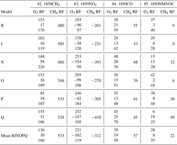
For example, for model B, the NOxexperiment (#3) yields

a methane lifetime of 11.60 yr, compared to the base year 2000s experiment (#1) value of 8.70 yr (Table 7). The longer lifetime reflects lower levels of OH due to the removal of NOxemissions. If this experiment had been carried out with

methane free to adjust, Eq. (1) indicates that methane would have responded by increasing from 1751 ppb to an equilib-rium level of 2531 ppb (Table 7), generating a radiative forc-ing of 261 mW m−2. Thus the methane radiative forcing as-sociated with NOxemission increases from the 1850s up to

the 2000s is −261 mW m−2 (Table 8). The associated

ex-−400 −200 0 200 400 600 800 Radiative forcing (mW m−2) Other NMVOC CO NOx CH4 Contribution to methane RF Contribution to ozone RF

Fig. 4. Radiative forcings (1850–2000, mW m−2) generated by emissions of methane, NOx, CO, NMVOC, and the interactions be-tween these emissions (“Other”), split into their methane and ozone components. Dots are the net RF for each emission, with error bars estimated from the individual uncertainties listed in Tables 10 and 11.

tra ozone forcing is −96 mW m−2. Adding this to the ozone forcing found directly from the NOx attribution experiment

(193 mW m−2)yields a net ozone forcing of 97 mW m−2for model B (Table 8).

We extend our analysis to include the impacts of CH4, CO

and NMVOC emissions on CO2 concentrations. All these

emissions oxidise to form CO2and therefore generate an

ad-ditional RF (Table 9 and Supplement). Other effects, such as impacts of methane on stratospheric H2O, or impacts of

changes in oxidants on secondary aerosol (Shindell et al., 2009), are not included in our analysis. We summarise the average results of all the models that ran the attribution ex-periments in Table 9.

The calculated RF for a change in methane concentration of 791 to 1751 ppb (i.e. the observed and prescribed methane change between the 1850s and the 2000s) is 427 mW m−2. This change in methane concentration has been produced

Table 8. Tropospheric ozone and methane radiative forcings (mW m−2)for each model and attribution experiments #2–5 relative to ex-periment #1 (year 2000s). For methane radiative forcings in exex-periments #2–5, an equilibrium [CH4] is calculated based on the diagnosed perturbation to the methane lifetime (Table 7); the RF is then calculated from the difference between the prescribed and equilibrium methane concentrations. For ozone radiative forcings, three numbers are given: the uppermost is the RF from the calculated ozone field (e.g., Fig. S5); the middle value is the inferred ozone RF associated with the methane adjustment to equilibrium; the lower number is the net ozone RF.

#2. 1850CH4 #3. 1850NOx #4. 1850CO #5. 1850NMVOC Model O3RF CH4RF O3RF CH4RF O3RF CH4RF O3RF CH4RF B 153 480 193 −261 38 55 37 9 17 −96 21 3 170 97 59 40 J 103 505 178 −231 29 53 29 0 16 −58 13 0 119 120 42 29 N 168 606 253 −393 48 68 15 32 58 −154 28 13 226 99 76 28 O 153 546 205 −270 36 39 42 6 36 −99 15 2 189 106 51 44 P 85 533 246 −305 35 61 38 36 18 −62 13 8 103 184 48 46 Q 155 526 252 −410 45 65 6 49 31 −147 25 19 186 105 70 25 Mean BJNOPQ 136 533 221 −312 39 57 28 22 30 −102 19 8 166 119 58 35

by the combined increases in emissions of CH4, NOx, CO

and NMVOCs. However, the sum of the RFs generated when these emissions are changed one at a time is only 300 mW m−2(Table 9). The remaining 127 mW m−2is due to non-linear interactions between species in the chem-istry models, in particular the effect of NOx changes on

the methane forcing is much larger when applied at 2000s methane levels compared to 1850s methane levels. The non-linearity of the radiative forcing calculations (square root de-pendence) acts in the opposite direction, tending to reduce the impact of NOxchanges.

For ozone RF, the non-linear interactions between emis-sions appear to be minor, as the linear sum of the ozone RFs from the CH4, NOx, CO and NMVOC experiments is equal

to the ozone RF for 1850–2000 (Table 9). Table 9 reports this for the mean of the six models, but the same linearity is also approximately found for individual models. Based on the six models that performed the attribution experiments, the mean percentage contributions to ozone RF are methane (44 %), ni-trogen oxides (31 %), carbon monoxide (15 %), non-methane volatile organic compounds (9 %) (Table 10). The values

found here are compared with the earlier work of Shindell et al. (2005, 2009) in Tables 10 (ozone) and 11 (methane).

As can be seen in Tables 10 and 11, there are some differ-ences between this work and the two Shindell et al. studies. For the tropospheric ozone RF, we find a smaller (but still dominant) contribution from methane emissions (the Shin-dell et al. (2005) result is within the range found in the AC-CMIP analysis), and a larger contribution from NOx

emis-sions. The contributions from CO and NMVOC emissions are less important, and more similar to the two Shindell et al. studies. For methane RF, all the studies find a rather sim-ilar contribution from methane emissions, and also from the CO and NMVOC emissions. However, the ACCMIP models have a more strongly negative contribution from NOx

emis-sions, and they show a significant non-linearity in that the net effect of all emissions does not sum to give the same RF as all emissions together. The emissions based RFs are sum-marised in Fig. 4.

1750 1800 1850 1900 1950 2000 2050 2100 Year 0 200 400 600 800 O3 RF / mWm -2 RCP8.5 RCP2.6 RCP6.0 RCP4.5

Fig. 5. Evolution of tropospheric ozone RF (mW m−2), 1750–2100. For 1750–1850, we show the estimate of Skeie et al. (2011). For 1850–2000 (black line), we show MMM values for all available AC-CMIP timeslices. For 2000–2100, the four RCP scenarios are shown in different colours, using values at 2030 and 2100 only. Estimated uncertainties of ±30 % on all values are indicated by the grey shad-ing, bounded by dotted coloured lines. Values have been scaled to the average of the MASKZMT and MASK150 tropopauses, and the three radiation schemes used (Edwards-Slingo, Oslo, and NCAR).

3.2 Other simulations

Several models ran time slice simulations covering several intervening decades between the 1850s and 2000s, and also for the four future Representative Concentration Pathway scenarios (RCP2.6, RCP4.5, RCP6.0 and RCP8.5) (Table 1). Young et al. (2013) provide details of the changes in surface and tropospheric ozone from these simulations. Here, we use spatially resolved annual mean changes in tropospheric column ozone, and convolve these together with individual model’s normalised ozone RFs (Fig. S2), to estimate the RF for each timeslice experiment relative to the 1850s (Fig. 5). A subset of these results (for the 1980s, 2000s, 2030s and 2100s) is also presented in Table 12. Seasonal variations in both column changes and normalised RFs are not accounted for, and this indirect method of calculating RFs also as-sumes that the normalised ozone RF for 1850s–2000s does not change with time; i.e. that the shape of the change in ozone vertical profile is temporally invariant. We consider that these approximations introduce only small errors in the estimates of ozone RF presented in Fig. 5 and Table 12.

Table 12 also shows mean values for selected time peri-ods, constructed in three different ways: (i) using all avail-able models for a given time slice; (ii) just using the four models (F, G, K and N) that ran all of the timeslices in Ta-ble 12; and (iii) using a subset of ten models (A, B, F, G, K, L, M, N, O and P) that ran all the time slices except those for RCP4.5 and RCP6.0. Comparing the mean values cal-culated by these different methods shows that there is little

Table 9. Emission-based RFs (for 1850s–2000s) (via changes in CO2, CH4 and tropospheric ozone) for emitted CH4, NOx, CO, and NMVOC, based on the mean response of the six models that conducted the attribution experiments (cf. IPCC-AR4 Table 2.13).

Radiative forcing (mW m−2)via: Emission CO₂ CH₄ O₃ CO₂+CH₄+O₃ CH4 18 533 166 717 NOx −312 119 −193 CO 87 57 58 202 NMVOC 33 22 35 90 Other factorsc 127 0 127 Total: 138 427a 378b 943 a_{The total methane RF is constrained to be 427 mW m}−2_{by the observed} increase in CH₄concentrations from the 1850s (791 ppb) to 2000s (1751 ppb), as prescribed in the models. This is then used with the other components to infer the RF due to “other factorsc_”

(127 = 427 − 533 + 312 − 57 − 22 mW m−2_). b_{The mean value for these models for the total O}

3RF for 1850s–2000s is 378 mW m−2, which indicates that no other factors are required to explain the O3RF.

c_{The “other factors” not estimated in our attribution experiments include: (i)} non-linear interactions between emissions (i.e. simple linear addition of the effects of individual species misses interactions that occur when species change together); and (ii) changes in the value of f between the 1850s and 2000s.

influence on the overall results (the maximum deviation is 24 mW m−2, or ∼ 10 %, for RCP6.0 in 2100) of the variable model coverage of different timeslices.

3.3 Experiments that isolate the climate change component

Most models performed the core 1850s and 2000s experi-ments with driving climates appropriate for these decades (Table 1). In addition, 10 models carried out sensitivity ex-periments with 2000s emissions, but driven by 1850s cli-mate. Most of these models also performed similar exper-iments, but driven by 2030s and 2100s climates (RCP8.5). By comparing runs with the same emissions, but different climates, we can diagnose the impact of climate change on tropospheric ozone. Figure 6 shows the impact of climate change on ozone, for the multi-model mean of the eight mod-els that performed all of the above experiments. Figure S7 shows results for individual models.

Modelled tropospheric ozone shows a range of responses to climate change. The largest overall response is seen in models G and H (the two GISS versions), where climate change is the main driver of the SH decreases in ozone seen in these models (Fig. S1). In these GISS integrations, the stratosphere also changes, so it is unclear if it is strato-spheric change or climate change that is driving the SH de-creases. The other model with large decreases in SH ozone (M), also changes its stratosphere in its climate change ex-periments, however the climate change experiment does not produce the large SH decrease seen in the standard 1850s–

Table 10. Contributions of emissions of CH4, NOx, CO and NMVOC to the 1850–2000 O3RF, in both absolute terms (mW m−2)and as percentages, for this study, and also from Shindell et al. (2005, 2009). The Shindell et al. (2005, 2009) values are all for 1750–2000, and are instantaneous RFs calculated using a different methodology. The ACCMIP values are the means and standard deviations of the six models in Table 8. The Shindell et al. (2005) values have estimated errors of ±20 % for CH4and ±50 % for other emissions.

Model range of emission contributions to tropospheric O3RF

Emission ACCMIP Shindell et al. (2005) Shindell et al. (2009) CH4 166 ± 46 mW m−2(44 ± 12 %) 200 ± 40 mW m−2(51 ± 10 %) 275 mW m−2(74 %) NOx 119 ± 33 mW m−2 (31 ± 9 %) 60 ± 30 mW m−2 (15 ± 8 %) 41 mW m−2 (11 %) CO 58 ± 13 mW m−2 (15 ± 3 %) – 48 mW m−2 (13 %) NMVOC 35 ± 9 mW m−2 (9 ± 2 %) – 7 mW m−2 (2 %) CO+NMVOC 93 ±10 mW m−2 (25 ± 3 %) 130 ± 65 mW m−2(33 ± 17 %) 55 mW m−2(15 %)

Table 11. Contributions of emissions of CH4, NOx, CO and NMVOC to the 1850–2000 CH4RF (mW m−2), for this study, and also from Shindell et al. (2005, 2009). The Shindell et al. (2005, 2009) values are all for 1750–2000, and were calculated with a different methodology. The ACCMIP values are the means and standard deviations of the six models in Table 8. The Shindell et al. (2005) values have estimated errors of ±20 % for CH4and ±50 % for other emissions.

Model range of emission contributions to CH4RF (mW m−2) Emission ACCMIP Shindell et al. (2005) Shindell et al. (2009) CH4 533 ± 39 590 ± 120 530 NOx −312 ± 67 −170 ± 85 −130

CO 57 ± 9 – –

NMVOC 22 ± 18 – –

CO+NMVOC 79 ± 26 80 ± 40 80

2000s experiment, so the origin of this signal in this model remains unclear. Some models show increases in tropical mid- to upper tropospheric ozone, with these increases cen-tred over the continents (G, H, and to a lesser extent O, F and L). All these models (except F) show (small) increases in lightning NOxemissions (Table 2); however, other

mod-els that also show increases in lightning do not show obvi-ous increases in tropical ozone (A, M, N and P). Most of the models show decreases in ozone, particularly in the tropical lower troposphere, which would be expected due to increases in water vapour and hence ozone destruction (e.g., Johnson et al., 2001; Doherty et al., 2013). Several models also show indications of increases in the stratospheric source of ozone, e.g., in the sub-tropical jet region (A, F, I, L, and P). Simi-lar features have been seen in some future simulations under climate change scenarios (e.g., Zeng and Pyle, 2003; Steven-son et al., 2006; Kawase et al., 2011). On average, the net impact of climate change on ozone is a small decrease in tro-pospheric ozone burden.

The net impact of climate change on tropospheric ozone RF is reported in Table 12. The multi-model mean suggests that the forcing is small and negative (−20 to −30 mW m−2), for both the present-day and in the future, i.e. there is a small negative climate feedback related to tropospheric ozone. This feedback is rather uncertain however, with some models in-dicating small positive feedbacks, and others showing the

sign of the feedback changing from negative for 1850 up to present day to positive for the future. These differences ap-pear to mainly reflect competition between the mechanisms outlined above.

4 Discussion and conclusions

With the MASKZMT tropopause, we find a mean value for the tropospheric ozone radiative forcing (1850s–2000s) of 356 mW m−2, with a standard deviation across 17 mod-els of ±58 mW m−2 (±16 %) (Table 12). The median model has a value of 371 mW m−2, and the full range spans 211–429 mW m−2. The model at the low end of this range (model M) is an isolated outlier – the next lowest value is 297 mW m−2 (Table 12). Using an alter-nate tropopause (MASK150), we find slightly higher val-ues: 377 ± 65 mW m−2(±17 %) (Table 3). Values from the two sets of calculations differ by 6 %; this suggests that tropopause definition introduces an uncertainty of at least

±3 %.

These values were calculated by the Edwards and Slingo (1996) (E-S) radiation scheme. We find that the E-S ra-diation scheme gives net, stratospherically adjusted ozone RFs that are 10 % higher than comparable schemes from Oslo and NCAR (Table 5). Taking the mean of our values

Table 12. Tropospheric ozone RFs (mW m−2)relative to the 1850s (for MASKZMT), calculated from column ozone changes and normalised RFs for each model. Values shown for some models in brackets under 2000s and for the RCP8.5 scenario are the impact of climate change on RF, with mean (±SD) values given in the last row. NB values for 2000s differ very slightly from Table 3 due to the masking of some normalised RF values. RCP2.6 RCP4.5 RCP6.0 RCP8.5 Model 1980s 2000s 2030s 2100s 2030s 2100s 2030s 2100s 2030s 2100s A 364 428(−27) 329∗ 150∗ – – 364∗ 229∗ 521(−26) 733(−23) B 307 384 345 164 406 262 – – 456 527 C 262 315 – – 341 202 – – 385 490 D 337 429 – – 439 308 – – – 680 E 312 365 – – – – – – – – F 365 407(−15) 367 195 443 328 439 335 513 (−2) 775(+31) G 275 297(−87) 293 184 330 235 325 301 420(−74) 567(−14) H 271 311(−47) – – – – – – – – I 227 302 (+2) – 150 – 270 – – – 570(+18) J – 316 – – – – – – – – K 279 345 280 123 355 237 307 227 391 484 L 302 377(+12) 323 177 – – 367 260 441(+13) 527(−39) M 190 211(−22) 191 106 – – 222 157 309(−26) 430(−87) N 337 406(−22) 338 156 402 261 353 230 449(−36) 587(−70) O 336 396(−31) 339 154 – – – – 468(−40) 560(−81) P 296 371 (−1) 367 253 427 356 – – 474 (−7) 637(+19) Q – 399 – – – – – – – – Mean ± SD (all) 297 ± 49 356 ± 58 317 ± 52 165 ± 39 393 ± 45 273 ± 49 340 ± 66 249 ± 58 439 ± 61 582 ± 100 Mean ± SD (FGKN) 314 ± 44 364 ± 53 320 ± 40 165 ± 32 382 ± 50 265 ± 43 356 ± 58 273 ± 53 443 ± 52 603 ± 123 Mean ± SD 305 ± 51 362 ± 65 317 ± 52 166 ± 40 – – – – 444 ± 62 583 ± 107 (ABFGKLMNOP) 1Climate −24 ± 27 −25 ± 25 −33 ± 42 Mean ± SD (AFGLMNOP)

∗_{Model A (CESM-CAM-superfast) RCP2.6 and 6.0 results used SST/SIC inconsistent with these scenarios.}

for the two different tropopauses with the E-S scheme (367 mW m−2), and adjusting for the Oslo and NCAR schemes producing slightly lower values (i.e. giving equal weight to each radiation scheme by multiplying by a factor of (1.0 + 0.9 + 0.9)/3 = 0.93), our best estimate of tropospheric ozone RF (1850–2000) is 343 mW m−2.

Based on a comparison of instantaneous clear sky SW ozone RFs between the E-S and Oslo schemes (Table 5), we estimate radiative transfer schemes introduce uncertainty of about ±6 %. Clouds influence ozone RFs to different degrees in the E-S and Oslo schemes, and add uncertainty of at least

±7 % (Table 4). The influence of stratospheric adjustment also varies between the two schemes, adding uncertainty of about ±3 %. Based on these individual uncertainties, and as-suming they are independent, we estimate an overall uncer-tainty associated with the radiation scheme of about ±10 %, based on the square root of the sum of the squares (RSS). Combining these uncertainties with the model range (±17 %) and difference due to tropopause definition (±3 %), we esti-mate an overall (RSS) uncertainty of ±20 % from these fac-tors.

Further sources of uncertainty in the ozone RF stem from uncertainties in precursor emissions (natural and anthro-pogenic), as well as changes in climate and stratospheric ozone. The partitioning of RF between tropospheric and stratospheric ozone may also change as tropopause height and morphology changes (Wilcox et al., 2012); we have not explicitly considered this impact on RF. Most models predict relatively small impacts on tropospheric ozone via climate change up to present-day, but these impacts may increase in future (Fig. S7). Uncertainties associated with these factors, and emissions in particular, are probably similar or larger than the ±20 % estimated above. We therefore estimate an overall uncertainty of ±30 % on our central estimate (Skeie et al. (2011) estimate the same value for uncertainty). Given the magnitude of the uncertainty, we quote values to two sig-nificant figures, giving our best estimate and uncertainty of 340 ± 100 mW m−2. It should be noted that this value is for 1850s to 2000s (which we take to be 1850 to 2000). Skeie et al. (2011) calculated tropospheric ozone increases between 1750 and 1850 of 1.0 DU (using model B), suggesting an ex-tra 42 mW m−2should be added to give the RF from 1750 to 2000. Similarly, they calculate an increase from 2000 to 2010