Dictionary-based output-space dimensionality
reduction
Pablo Strasser1,2
[email protected] Jun Wang
1
[email protected] Stéphane Armand
3
Alexandros Kalousis1,2
1Department of Business Informatics
University of Applied Sciences Western Switzerland
2Computer Science Department
University of Geneva Switzerland
3Willy Taillard Laboratory of Kinesiology
Geneva University Hospitals and Faculty of Medicine
Switzerland
Abstract
In this paper we propose a method for output dimensionality reduction based on dictionary learning. Our final goal is the prediction of complete time series from standard input vectorial data. To do so we formulate a single learning problem which on the one hand learns a new representation of the output space, using dictionary learning, and reduces its dimension, while on the other hand learns to predict from the input data the new output representation, using standard multi-output regression. As a result the choice the new representation is informed by the prediction error, and the regression model by the reconstruction error. We provide preliminary experiments which demonstrate the potential of our approach and discuss its limitations.
1 Introduction
In this paper we explore the problem of supervised learning where the output is a time series. More precisely we are given instances from some traditional vectorial input space, where each instance is coupled with a time-series vector. We want to learn a model that will accurately predict the time-series associated with a given instance given only its input space description. To do so we learn a new lower dimensional representation of the output space using dictionary learning tools, [6, 7, 10, 1]. The prediction problem is now defined over the lower dimensional space, given by the coefficients of the instances with respect to the learned basis, and the goal is to learn a predictive model that will take us from the input space to the new output representation. Given a test instance, once we obtain its predicted output representation we can go back to the original output representation using the learned dictionary basis. We define a single learning problem in which we optimize on the same time over the dictionary and the predictive model. The result of this single step optimization is that we directly find a new output represenation that is most appropriate
Published in proceedings of the Neural Information Processing 2013, Workshop on
Output Representation Learning, p. 1-6 which should be cited to refer to this
work
for the predictive task that we have to address. We perform preliminary experiments on a real world dataset in which the goal is to predict the gait of a patient from his/her clinical description and discuss our findings.
2 Related Work
A related line of research is the work on structured output prediction in which the target variable is a discrete structure object, such as a tree, a ranking, an alignment etc [9]. A more directly related line of work is the more recent work on multi-label classification problems. In a multi-label classification problem an instance is associated with one, or more, class labels from a fixed set of classes, resulting in a target variable that is defined in the {0, 1}mspace,
where m is the total number of classes. One of the recently proposed ways to solve such problems is through a change of representation in the output space, which typically, but not always, will lead to a new output space of smaller dimensionality. The new representation is chosen so that it will result in an easier prediction problem. Most of the work that follows this approach, [3, 5, 8, 11, 12], can be seen as consisting of three distinct steps. An encoding step in which we learn a new output representation, a prediction step in which we learn a model that given the input description of an instance learns its new output representation, and a final decoding step which maps back from the predicted representation in the new output space to the representation in the original output space. The different approaches differ on how they model each of the constituent steps and how the defining the optimization problem, e.g. a sequence of optimization problems, solved one after the other, or a single one.
All of the above work concerns discrete output spaces with feature values in {0,1}. Unlike them our output space is continuous in which consecutive features have a high correlation, since they form a time-series. We thus need a more appropriate way to achieve dimension-ality reduction in our time-series output space.
3 Methodology
Similarly to the situation in multilabel classification, our goal is to learn accurate mappings from the input space to the time-series output space. The time-series are considered as a vec-tor of same time measurement or interpolation. In our case, the time-series are continuous enough and sufficiently well sampled to be able to ensure this by interpolation if needed. In order to achieve that instead of trying to directly predict the multi-dimensional time-series output we will first learn a compression to a new low-dimensional representation for the time-series using dictionary learning [4].Thus we will learn a new basis for the output space and the respective coefficients for the learning instances. These coefficients will become the new prediction target, which we will predict with the help of some regression model. In testing time once the coordinates of some instance in the new output space are available we will reconstruct its respective signal in the original output space using the learned basis. We should note that the method which we will present learns on the same time both the dictionary basis and the regression model. The result of this interdependency is that the learned representation is more appropriate for the prediction, since itself is established as a part of the supervised learning process.
Before proceeding to the description of the method let us introduce some notation. We are given n input learning instances xi∈ X = Rd. Each instance xiis associated with its target
time-series vector yi∈ Y = Rm. We denote by X ∈ Rn×dthe input feature matrix, the ith
line of which is the xT
i input feature vector, and by Y ∈ R
n×mthe output matrix the ith line
of which is the output time-series vector yT
i. The overall goal is to learn some function f()
which given an input vector x will produce its respective time-series vector y. The simplest such function would be the multi-output regression function of the form WTx, W : d × m.
3.1 Output space dimensionality reduction
As we already mentioned to reduce the dimensionality of the output space we will rely on dictionary learning and we will use as the new representation the learned coefficients. In dictionary learning we find a new basis, which will consist of what we may call “proto-typical” time-series, linear combinations of which describe well the output space Y. Thus in dictionary learning we learn a basis matrix B : q × m, the rows of which are the new basis, together with a coefficient matrix C : n × q, the i row of which is the new output representation of the i instance, such that:
Y = CB. (1)
To avoid overfitting one needs to regularize the learned coefficient matrix typically using the `1 of C. Thus the optimization problem that one solves in dictionary learning is:
arg min C,B LD(C, B) = Xij Yij− X k CikBkj !2 + λD`1(C), s.t. ||Bi||2= 1 ∀i. (2) where λD controls the reconstruction-error and regularization trade-off and the l2 norm
constraint on the Bi lines is used to avoid scaling problems, and have a unique solution.
Thus the new output representation of the ith instance will be given by the ith row of C,
ci, and our goal will now be to predict ci from xisolving what is essentially a multi-output
regression problem.
3.2 Multi-output regression
To solve the multi-output regression problem we will use standard multi-output regression, and solve the following optimization problem :
arg min W LR(W) = Xij Cij− X k XikWkj !2 + λR`2(W), (3)
where W : d × q is the multi-output regression coefficient matrix, and λR controls the
prediction-error and regularization trade-off. Once the regression model is learned we can predict the output time-series of an instance x by:
ˆ
y = BTWTx. (4)
Note that the multi-output regression is easy to kernelize.
3.3 Supervised output space dimensionality reduction
The easiest way to learn a function that will predict the output series given the input description is to to first solve the dictionary learning problem, eq 2, to find the new output representation and then solve the multi-output regression problem given in eq 3 over the representation learned in the previous step. However the disadvantage of such a sequential approach is that it does not exploit any supervised information in learning the new output representation. The learned basis might not be optimal for the prediction task that we have to solve. A more appropriate way is to couple the two optimization problems to define a single one which we will solve in one step. Under such a strategy the learning of the basis will be supervised through the prediction task, making explicit the fact that the new representation should be easy to predict from the input vector, thus leading to the learning of a more appropriate basis for the output space. By combining the two optimization problems given in eqs. 2, 3 we get the following problem optimization problem:
arg min W,C,B L(W, C, B) = Xij Cij− X k XikWkj !2 + λR`2(W) + λX ij Yij−X k CikBkj !2 + λD`1(C), s.t. ||Bi||2= 1. (5)
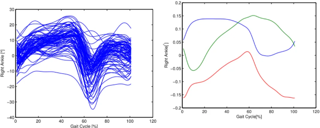
0 20 40 60 80 100 120 −40 −30 −20 −10 0 10 20 30 Gait Cycle [%] Right Ankle [ ° ]
Figure 1: Sample of the time series.
0 20 40 60 80 100 120 −0.2 −0.15 −0.1 −0.05 0 0.05 0.1 0.15 0.2 Gait Cycle[%] Right Ankle[ °]
Figure 2: Dictionary learned in the out-put space (Sequential case).
λ trades-off between the prediction error and the output space reconstruction error. As λ → 0 the regression problem will be more important and the dictionary choice will only matter in case of ambiguity. As a result the C matrix will be in the set of the exactly predictable outputs of the regression, within which the dictionary method will choose the best solution. More concretely for the linear regression, it will choose an C in the image of the design matrix X. As λ → ∞ the dictionary will be more important and the regression loss will be used only in case of ambiguity. This is equivalent to sequential learning where we first learn the dictionary and then solve the regression problem. Under this approach if in the dictionary learning step we could find the set of all global minima then the regression step over them would select the final best solution.
3.4 Optimisation strategy
We will use an iterative strategy optimizing one variable at the time while keeping the others fixed. When solving the dictionary part, we need to impose the norm constraint on every word of the dictionary. This is done by using a steepest descend with Armajilo line search where every new dictionary is normalized. The complete algorithm will converge to a local minima because at every step we are ensured to reduce the value of the loss function.
4 Experiments and discussion
We will evaluate our method on a real world dataset on a gait prediction problem for patients with a cerebral palsy. The input features constitute a 36-dimensional vector and they are the results of clinical examinations. The output for each patient is a 101-points time series, spanning one gait cycle, giving the angle that the right ankle forms at each time point. We have a total of 145 patients. This is a quite challenging problem and the current work is the first one that tries to address it.
We estimate performance with hold out testing. We randomly select 108 instances for training and 37 for testing. Moreover we split the training set in a learning set, 81 instances, and a validation set, 27 instances. We use the latter to tune the different hyperparameters, namely λD, λR, λ. Our evaluation measure is the mean sum of squares of the prediction
error. All the output features were standardised to a mean of zero and a standard deviation of one.
We experimented with our method in two different modes. In the first one, which we will call the sequential, we use two distinct steps, first fitting the dictionary, and then solving a multi-output regression problem on the new representation; as already mentioned before this is equivalent to λ → ∞, we will call this seq-D-MOR. In addition to the seq-D-MOR we also experimented with ν-SVM as the regression algorithm [2] learning its output independently. We used the RBF kernel where γ ∈ {10−k|k = 1 . . . 6}was chosen in the validation set, we
Method #-basis λ λR λD c γ Mean square error Impr. to median Median − − − − − − 6.7 · 103 0% MOR − − 400 − − − 5.8 · 103 14% seq-D-MOR 3 − 100 1 − − 5.1 · 103 23% seq-D-ν-SVM 12 − − 300 0.7 10−6 6.5 · 103 3% D-MOR 3 300 30 300 − − 5.1 · 103 23% seq-D-R-MOR 8 − 100 1 − − 5.4 · 103 19% seq-D-R-MOR 3 − 100 1 − − 5.2 · 103 22%
Table 1: Results summary, and parameter settings chosen in validation set.
C.f fig. 1 for an example of the output space, and C.f fig. 2 for a visualisation of the dictionary.
In the second one, we directly solve the optimization problem given in eq. 5; we will denote this method by D-MOR. We tune the three different trade-off parameter (λ, λR, λD) by
selecting values in the set {0, 0.001, 0.1, 1, 10, 1000} and the number of dictionary basis in the set {3, 7, 9, 11, 13} using the validation set performance. To refine the value of the trade-off parameter, we searched around the solution of the first exhaustive grid search. To test if we had local minima, we did multiple restarts that give very similar results.
D-MOR achieves a better result compared to MOR, which show that the compression ac-tually helps the prediction. The poor performance of ν-SVM can be explained by the fact that we did not use a multi-output SVM, but instead fit one ν-SVM per output dimension. We note that dictionary methods coupled with regression led to a selection of only three basis vectors, using the validation set performance. This is a further sign that linear regres-sion is not able to adequately exploit the information in the learned representation; in fact, surprisingly, as we saw it prefers less basis than more which would have led to a smaller reconstruction error. On the other side ν-SVM by ignoring the relations between the fea-tures of the new representation chooses a higher number of basis vectors. Another puzzling fact was that we did not obtain a better result with the single step learning compared to sequential learning. However, given the flexibility of the former we do expect to be able to achieve better performance, in this and similar datasets. Another interesting observation is that if we simply learn the dictionary, reconstruct the output signal according to the learned dictionary and coefficient, and predict directly the reconstructed signal using MOR we achieve better result than using directly MOR (We called this seq-D-R-MOR). As the number of dictionary basis reduces, the performance of seq-D-R-MOR improves. A fact that shows that the information we are removing when we use less basis is probably detrimental, e.g. noisy fluctuations. This is not only the case of seq-D-R-MOR but of all the methods that make use of the structure, D-MOR, seq-D-MOR, all of work better with less basis. At the end what we are probably observing is a regularization effect of the number of basis. An important difference between the MOR and the dictionary-based methods is that the former can be seen as a local method in which we learn a model for each output dimension independently, and connect them only through the final prediction error, while in the latter the basis vectors span the full output, and can thus be seen as a global method. In any case these are very preliminary observations. We still need to do much more thorough and extensive experiments, refining the experimental methodology, and study the effect of the different parameters with an emphasis on the dictionary size.
In addition to the further experiments and a thorough study on the effect of the dictionary size we will also derive a kernelized version of the method we proposed here, to address the non-linear effects of dictionary learning. We want also to define an hierarchical dictionary learning structure in which we will have a second level dictionary learning that will provide more refined representation information over the first.
References
[1] Krishnakumar Balasubramanian and Guy Lebanon. The landmark selection method for multiple output prediction. pages 983–990, 2012.
[2] Chih-Chung Chang and Chih-Jen Lin. LIBSVM: A library for support vector machines. ACM Transactions on Intelligent Systems and Technology, 2:27:1–27:27, 2011. Software available at http://www.csie.ntu.edu.tw/~cjlin/libsvm.
[3] Yao-Nan Chen and Hsuan-Tien Lin. Feature-aware label space dimension reduction for multi-label classification. In Peter L. Bartlett, Fernando C. N. Pereira, Christopher J. C. Burges, Léon Bottou, and Kilian Q. Weinberger, editors, NIPS, pages 1538–1546, 2012.
[4] M. Elad and M. Aharon. Image denoising via sparse and redundant representations over learned dictionaries. Image Processing, IEEE Transactions on, 15(12):3736–3745, 2006.
[5] Daniel Hsu, Sham Kakade, John Langford, and Tong Zhang. Multi-label prediction via compressed sensing. In Yoshua Bengio, Dale Schuurmans, John D. Lafferty, Christopher K. I. Williams, and Aron Culotta, editors, NIPS, pages 772–780. Curran Associates, Inc., 2009.
[6] Julien Mairal, Francis Bach, Jean Ponce, and Guillermo Sapiro. Online dictionary learning for sparse coding. In Proceedings of the 26th Annual International Conference on Machine Learning, ICML ’09, page 689–696, New York, NY, USA, 2009. ACM. [7] Julien Mairal, Francis Bach, Jean Ponce, Guillermo Sapiro, and Andrew Zisserman.
Supervised dictionary learning. arXiv:0809.3083, September 2008.
[8] Farbound Tai and Hsuan-Tien Lin. Multilabel classification with principal label space transformation. Neural Computation, 24(9):2508–2542, 2012.
[9] Ioannis Tsochantaridis, Thorsten Joachims, Thomas Hofmann, and Yasemin Altun. Large margin methods for structured and interdependent output variables. Journal of Machine Learning Research, 6:1453–1484, 2005.
[10] Yangmuzi Zhang, Zhuolin Jiang Vlad I. Morariu, and Larry S. Davis. Learning struc-tured low-rank representations for image classification. In CVPR, 2013.
[11] Yi Zhang and Jeff Schneider. Maximum margin output coding. In ICML. icml.cc / Omnipress, 2012.
[12] Yi Zhang and Jeff G. Schneider. Multi-label output codes using canonical correlation analysis. Journal of Machine Learning Research - Proceedings Track (AI-STATS), 15:873–882, 2011.