HAL Id: hal-02906584
https://hal.archives-ouvertes.fr/hal-02906584
Submitted on 25 Jul 2020
HAL is a multi-disciplinary open access
archive for the deposit and dissemination of
sci-entific research documents, whether they are
pub-lished or not. The documents may come from
teaching and research institutions in France or
abroad, or from public or private research centers.
L’archive ouverte pluridisciplinaire HAL, est
destinée au dépôt et à la diffusion de documents
scientifiques de niveau recherche, publiés ou non,
émanant des établissements d’enseignement et de
recherche français ou étrangers, des laboratoires
publics ou privés.
Distributed under a Creative Commons Attribution - NonCommercial - NoDerivatives| 4.0
International License
Brillouin mirror with inverted acoustic profile in
presence of strong acoustic dispersion
Antonio Montes, Carlos Montes, Éric Picholle
To cite this version:
Antonio Montes, Carlos Montes, Éric Picholle. Brillouin mirror with inverted acoustic profile in
presence of strong acoustic dispersion. Journal of the Optical Society of America B, Optical Society
of America, In press. �hal-02906584�
Brillouin mirror with inverted acoustic profile in
presence of strong acoustic dispersion
A
NTONIOM
ONTES,
1C
ARLOSM
ONTES,
2 ANDÉ
RICP
ICHOLLE 2,*1Department of Applied Mathematics II (MA2), Universitat Politècnica de Catalunya, Barcelone, Spain 2Institut de Physique de Nice (INPHYNI), UMR 7010 Université Côte d’Azur & CNRS, Parc Valrose, 06108
Nice cedex, France
*eric.picholle@inphyni.cnrs.fr
Abstract: While usually negligible in standard optical fibers, the group velocity dispersion of
acoustic waves may in some cases play a significant role in the dynamics of stimulated Brillouin scattering (SBS) in propagation medias with more complex structures, such as microstructured fibers. The usual 3-wave coherent model of SBS can be adapted to take a perturbative acoustic dispersion into account, but the slowly varying envelopes approximation does not hold for stronger values of the acoustic dispersion, which call for a more sophisticated inertial model of SBS. A new regime of SBS mirror with a spatially inverted acoustic profile is predicted in this limit. In presence of strong acoustic dispersion, this regime exhibits a higher conversion efficiency than the usual mirror in the dispersionless case, as well as nonlinear self-stabilization of the phase of the acoustic wave when the pump is strongly depleted. Formal calculations allow the identification of regions of strong dynamic dispersion.
1. Introduction
Stimulated Brillouin scatttering (SBS) could once appear as a very well understood nonlinear phenomenon in optical fibers and waveguides, with a robust coherent three-wave model [1, 2] fully accounting for its extremely rich dynamics in 1D-media such as single-mode silica optical fibers (SMF). Indeed, besides the common ’SBS mirror’ [3, 4], both self-stabilized ultracoherent regimes [5–8], bifurcations [9] and bistability [10], soliton regimes [6, 11], SBS chaos [12, 13] and even SBS rogue waves [14, 15] in SMFs are well described by this 3-wave model.
Nevertheless, a kind of ’renaissance in Brillouin scattering research’ could recently be heralded [16], with a remarkable extension of the realm of Brillouin lasers in numerous and varied new kinds of waveguides, including microstructured fibers, silica [17] or chalcogenide [18], but also multicore fibers [19], micro- and nano-fibers [20, 21], hollow core PCFs [22, 23] as well as silicon [24] and silicon nitride [25, 26] waveguides, optomechanical waveguides [27] and even on-chip SBS laser devices [28].
In particular, the growing technological importance of photonic crystal fibers (PCF) yielded special interest on the acoustical properties of small-core PCFs, which microstructuring substan-tially changes the acoustic dispersion relation, and even the general acoustic properties [29–32] compared to conventional single-mode fibers.
Recent advances in cavity optomechanics also allowed to design tight confinement structures with acoustic dispersion values that deviate substantially from the usual linear dispersion relation of bulk materials or traditional SMFs [33], or even nontrivial topological acoustic band structures at interfaces [34]. A direct corollary is that some tightly confined acoustic modes may present a finite cutoff frequency, yielding a flat, Raman-like acoustic dispersion relation 𝜔𝑎(𝑘𝑎) [19,25,29], that is, a strong acoustic group velocity dispersion near cutoff.
The aim of this article is to explore the consequences of the acoustic dispersion on the 1D dynamics of SBS. After showing that even perturbative values of this dispersion, still compatible with an adaptation the usual 3-wave model (§3), can in some cases induce quite significant effects, we will consider the consequences of a stronger acoustic dispersion. We show that, relaxing the slowly varying envelopes (SVE) approximation, a new SBS mirror regime with an
inverted acoustic profile and a low threshold can be predicted through a more complete inertial 3-wave model of SBS, and we discuss its specific features (§4). Finally, we will identify potential regions of strong dynamic acoustic dispersion (§5). An Appendix considers the quite complicated acoustic dispersion relation in the inertial limit.
2. Dispersionless case
2.1. Standard coherent 3-wave model of SBS
The now standard 3-wave model for SBS optical fibers [1, 2, 35, 36] and, more recently, for some optomechanical cavities [37] was originally derived from the coherent model of SBS in laser-plasma interactions [38–41]. It is usually assumed that the slowly varying envelopes approximation holds for both optical waves (pump and Brillouin, of respective frequencies 𝜔𝑝 and 𝜔𝐵), as well as for the acoustic wave, of frequency 𝜔𝑎, as long as nanosecond or longer pulsed regimes, or a fortiori stationary or quasi-stationary regimes, are considered. In the 1D (or quasi-1D) approximation, the coupled evolution equations for the pump (𝐸𝑝), backscattered Brillouin (𝐸𝐵), and acoustic (𝐸𝑎) complex amplitudes read :
(𝜕𝑡+ 𝑐/𝑛 𝜕𝑥+ 𝛾𝑒) 𝐸𝑝= −𝐾𝑆 𝐵 𝑆𝐸𝐵𝐸𝑎 (1) (𝜕𝑡− 𝑐/𝑛 𝜕𝑥+ 𝛾𝑒) 𝐸𝐵= 𝐾𝑆 𝐵 𝑆𝐸𝑝𝐸 ∗ 𝑎 (2) (𝜕𝑡+ 𝑐𝑎𝜕𝑥+ 𝛾𝑎) 𝐸𝑎= 𝐾𝑆 𝐵 𝑆𝐸𝑝𝐸 ∗ 𝐵 (3)
where the material density 𝜌 is dimensioned to an equivalent electric field through 𝜌 = 𝑖𝜎𝐸𝑎, with 𝜎2= 𝜌0𝑛3𝜀0
2𝑐𝑐𝑎 , 𝛾
𝑒and 𝛾𝑎are the optical and acoustical losses coefficients, respectively, 𝑛 is the effective optical index (usually considered identical at both pump and Brillouin frequencies for numerical simulations, but distinct values can easily be taken into account) and 𝑐𝑎the effective phase velocity of the considered acoustic mode.
𝐾𝑆 𝐵 𝑆 = r
𝜀0𝑛7𝑝2
12
8𝜌0𝑐𝑎𝑐
𝜔𝑝 is the SBS coupling coefficient, with 𝑝12 the effective elasto-optic coefficient of the material [1]. Additional terms in Eq. (3) can account for the initiation of SBS from thermal noise [2], and in Eqs. (1 &2) for a perturbative optical Kerr effect [1].
Let us emphasize that, since SBS is a coherent 3-wave process, the energy transfers can happen both ways (i.e. Stokes process : creation of a Brillouin photon and an acoustic phonon at the expense of a pump photon; antiStokes : creation of a pump photon by recombination of a Brillouin photon and an acoustic phonon), depending on the relative phases of the three waves. More precisely, the gain is locally proportional to 𝑐𝑜𝑠 Φ, where Φ = 𝜑𝑝− 𝜑𝐵− 𝜑𝑎, and 𝜑𝑝 , 𝐵 , 𝑎 are respectively the phases of the pump, Brillouin and acoustic waves.
The acoustic propagation term in Eq. (3) is often neglected for simplicity, at the cost of superimposing an arbitrary gain linewidth that otherwise can be directly derived from system (1-3) in the stationary regime [42, 43].
The 1D approximation generally holds regardless of the polarization of the acoustic mode as long as only one such mode at the time is considered [44], typically in SBS lasers or amplifiers. Few-mode operation, either optical or acoustical, can still be taken into account in a quasi-1D approach by introducing additional coupled equations, allowing for instance to describe the coupling between longitudinal and radial or torso-radial acoustic modes in SMFs [45–47] or in hollow-core PCFs [22]. Nevertheless, the situation becomes intrinsically 3D when a continuum of bulk elastic waves must be considered [44].
2.2. Common SBS mirror
In the full (phases as well as amplitudes) stationary approximation, the 3-wave coherent model can be reduced to a 2-wave (pump & Brillouin) ’intensity model’ by re-injecting 𝐸𝑎 = 𝐸𝑝𝐸
∗
𝐵/𝛾𝑎) into Eqs. (1 & 2), whose long-known stationary solution [3, 4] is known as a ’SBS mirror’ [35, 36, 42].
In this regime, the intensities of the three waves (𝐼𝑝 , 𝐵 , 𝑎(𝑥) = |𝐸𝑝 , 𝐵 , 𝑎(𝑥) |2) monotonously decrease from their maximum value at the fiber end closest to the pump laser (left in Fig. 1). When the optical losses can be neglected, the counterpropagating pump and Brillouin waves are parallel (𝐼𝑝(𝑥) − 𝐼𝐵(𝑥) = 𝐶𝑠𝑡), the slave acoustic wave 𝐼𝑎(𝑥) ∝ 𝐼𝑝(𝑥) 𝐼𝐵(𝑥) following a similar distribution (Fig. 1).
Fig. 1. Common (dispersionless, 𝛼 = 0) SBS mirror: Spatial distribution of the amplitudes of the three waves (numerical, the dimensionless abscissa is the reduced fiber length 𝑥 −→ 𝑥/Λ = 𝑛𝐾𝑆 𝐵 𝑆
q
𝐼0𝑝𝑥/𝑐; 𝐺 = 14.5; 𝐿/Λ = 30, 𝜇 = 4.24, √
𝑅 = 0.091, 𝑡/𝑡𝑟 =25.46). Note that the intensities of all three waves monotonously decrease from the laser input end (left).
Further neglecting the pump depletion would yield an exponential amplification of the Brillouin wave : 𝐼𝐵(𝑥) = 𝐼 𝐿 𝐵𝑒 𝑔𝑆 𝐵 𝑆𝐼 0 𝑝( 𝐿−𝑥)where 𝑔 𝑆 𝐵 𝑆= 𝑛𝐾2 𝑆 𝐵 𝑆 𝑐 𝛾𝑎 is the SBS gain. 𝐺 = 𝑔 𝑆 𝐵 𝑆𝐼0𝑝𝐿is also a useful dimensionless gain parameter [1].
Nevertheless, the intensity model cannot describe the coherent properties of SBS, such as the finite width of the gain profile centered around the resonant SBS frequency 𝜔𝑟 𝑒𝑠
𝐵 defined by the phase-matching conditions kp =kresB + kresa and 𝜔𝑝 = 𝜔
𝑟 𝑒𝑠 𝐵 + 𝜔 𝑟 𝑒𝑠 𝑎 , where 𝑘𝑝= 𝑛𝜔𝑝/𝑐, 𝑘𝑟 𝑒𝑠 𝐵 = 𝑛 𝜔 𝑟 𝑒𝑠 𝐵 /𝑐 and 𝑘 𝑟 𝑒𝑠 𝑎 = 𝜔 𝑟 𝑒𝑠 𝑎 /𝑐𝑎.
When the stationary phase approximation is relaxed to allow off-resonance interaction [42, 43], the coherent 3-wave model yields in the single-frequency seeded SBS amplifier configuration the traditional lorentzian gain profile of width (FWHM) 𝛾𝑎.
When the SBS amplification starts from the acoustic noise [2], the reflectivity 𝐼0𝐵/𝐼 0 𝑝of the mirror becomes significant for large enough gains (typically, 𝐺 > 21 in standard SMFs [35]), depending also on the fiber modal structure and strain distribution [48]. In a SBS laser, the efficiency of the common SBS mirror is determined by the boundary conditions, the output Brillouin intensity being usually higher than the input pump intensity. Typically, the common SBS mirror shown in Fig. 1 presents a reflectivity of 75% for a gain 𝐺 = 14.5.
3. SBS in presence of weak acoustic dispersion
3.1. 3-wave model with perturbative acoustic dispersion
While the issue of the acoustic group velocity dispersion in fibers is a well-known problem in guided acoustics [49, 50], including in the context of SBS in microstructured fibers where specific
losses may strongly affect the acoustic dispersion relation [31, 51], it has mostly been applied to specific metrology applications [52].
In order to consider its influence on the SBS dynamics, a first approach is to adapt the coherent 3-wave model by integrating in the acoustic Eq. (3) an additional perturbative term 𝑖 𝛽𝑎𝜕𝑡 𝑡, where 𝛽𝑎 = 𝑐𝑎
𝑑2𝑘𝑎
𝑑 𝜔𝑎
2 1 is the acoustic group velocity dispersion coefficient, yielding:
(𝜕𝑡+ 𝑐𝑎𝜕𝑥+ 𝑖 𝛽𝑎𝜕𝑡 𝑡+ 𝛾𝑎) 𝐸𝑎 = 𝐾𝑆 𝐵 𝑆𝐸𝑝𝐸 ∗
𝐵 (4)
3.2. Stationary SBS mirror
In the full stationary approximation, 𝜕𝑡 𝑡𝐸𝑎=0 and the SBS mirror solution [3, 4] is obviously identical for both models with [Eqs. (1, 2 & 3)] and without [Eqs. (1, 2 & 4)] acoustic dispersion. The SBS gain remains unchanged. Taking into account both first order optical and acoustical dispersion yields a somewhat more complicated form of the gain profile of SBS amplifiers when the intensities are constant but not the phases, with:
𝑔𝑆 𝐵 𝑆(Ω) = 𝛾2 𝑎 𝛾𝑎2+ [(𝑘0𝑎+ 𝑘0𝑒) Ω]2 𝑔𝑟 𝑒𝑠 𝑆 𝐵 𝑆 (5) where 𝑔𝑟 𝑒𝑠
𝑆 𝐵 𝑆 is the usual SBS gain at resonance; Ω = 𝜔𝐵− 𝜔 𝑟 𝑒𝑠 𝐵 = 𝜔 𝑟 𝑒𝑠 𝑎 − 𝜔𝑎; 𝑘 0 𝑎𝑐 𝑟 𝑒𝑠 𝑎 = 1 − 𝜔𝑟 𝑒𝑠 𝑎 𝜕𝑐𝑎 𝜕 𝜔𝑎 |𝜔𝑎𝑟 𝑒𝑠; and 𝑘 0 𝑒𝑐= 𝑛 + 𝜔 𝑟 𝑒𝑠 𝐵 𝜕𝑛 𝜕 𝜔𝐵 |𝜔𝑟 𝑒𝑠 𝐵 .
It is interesting to note that the maximum value of the gain, at resonance, is not modified, but that this expression predicts an almost flat SBS gain whenever (𝑘0𝑎+ 𝑘
0 𝑒) = 0, i.e. 𝜆𝐵 ≈ 𝑐𝑎 2 𝜋( 𝜕𝑛 𝜕 𝜔𝐵 − 2𝑛 𝜕𝑐𝑎 𝜕 𝜔𝑎).
3.3. Dynamics of SBS solitons in presence of weak acoustic dispersion
Like single-mode fiber SBS lasers [6], PCF lasers with small enough feedback [9] exhibit pulsed solitonic behaviours. Our reference will be the experiment by Woodward et al. [17], where a SBS linear cavity is constituted by the small Fresnel reflexions at both ends of a 9m-long PCF fiber with a 3𝜇𝑚 core and an hexagonal structure of 0.7𝜇𝑚 air holes spaced by 1.9𝜇𝑚, yielding an effective area of 4.73𝜇𝑚2at the pump wavelength 𝜆𝑝 = 532𝑛𝑚. For pump powers between 57 and 123𝑚𝑊, they observed stable solitonic outputs, either sub- or superluminal, with pulses widths (FWHM) of 14.5 𝑛𝑠𝑒𝑐 ± 1.5 𝑛𝑠𝑒𝑐 [53]. This 10% fluctuation in soliton width could not be simply interpreted in the frame of the dispersionless 3-wave model.
Although neither the acoustic dispersion of the PCF fiber used in this experiment, nor a fortiori its dependence on the pump wavelength, has been determined, a possible interpretation of this fluctuation would make it a consequence of a steep dispersion relation of the involved acoustic mode.
Thus, we performed numerical simulations of the Woodward experiment through the 3-wave model both without [Eqs. (1,2 & 3), 𝛽𝑎 =0] and with [Eqs. (1,2 & 4), 𝛽𝑎 =0.01] perturbative acoustic dispersion. The normalized SBS gain was set at 𝐺 = 10.5, corresponding to an injected pump power 𝐼𝑝of about 100𝑚𝑊, and the small (intensity) reinjection coefficient
√
𝑅=0.091, ensuring a dynamics well into the solitonic region [10].
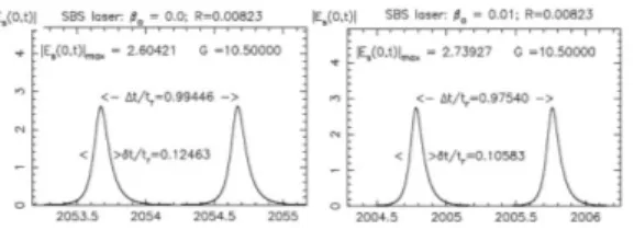
As expected, both simulations yielded stable solitonic outputs (Fig. 2), in sound qualitative agreement with the experiment, but with quite different quantitative features. Indeed, all other parameters being identical, the dispersionless model yielded almost luminal (𝑣𝑠𝑖 𝑔𝑛 𝑎𝑙=1.005 𝑐/𝑛) with a width (FWHM) around 5 𝑛𝑠𝑒𝑐, or 0.125 linear roundtrip time [Fig. 2, left], while 𝛽𝑎=0.01 yielded slightly faster (𝑣𝑠𝑖 𝑔𝑛 𝑎𝑙=1.025 𝑐/𝑛), but significantly compressed pulses, with a width of 4.6 𝑛𝑠𝑒𝑐 [Fig. 2, right], or a compression factor of 15 %. These value roughly corresponded to the extreme experimental values for the largest and slowest, and most narrow and fastest observed pulses, respectively.
A perturbative acoustic dispersion value thus appears sufficient to induce significant changes in the dynamics of a SBS laser, allowing typically for the possibility of a 10 to 15% variations in the SBS solitons temporal width, and a 2% velocity variation in such devices for 𝛽𝑎variations of the order of 1% from run to run, depending for instance on the exact pump wavelength or even on room temperature fluctuations.
Fig. 2. Output of a soliton laser (numerical, coherent 3-wave SVE model for a gain 𝐺 =10.5,
√
𝑅=0.091). Left: Amplitude 𝐸𝐵(0, 𝑡) of the Brillouin output without dispersion (𝛽𝑎 =0), the soliton travel at almost luminal velocity (𝑣 = 1.005 𝑐/𝑛); right: idem, but taking into account a perturbative acoustic dispersion (𝛽𝑎=0.01), the velocity slightly increases (𝑣 = 1.026 𝑐/𝑛) while the solitons are compressed by about 15%. (numerical. The parameters correspond to those of the experiment described
in [17].)
4. Inertial model of SBS in presence of strong acoustic dispersion
4.1. Inertial model
A key feature of the acoustic wave produced through the stimulated Brillouin process is its long lifetime, typically in the 10 ns range, well above the duration of the optical pulses used in telecommunications, yielding for instance long range interaction between the latter in fiber telecommunications [54,55]. A soliton train is best described by a standard nonlinear Schrödinger (NLS) equation whose solutions are injected as source input in Eq. (1) [56].
A similar procedure can be followed to take into account a strong acoustic group velocity dispersion. When the slowly varying envelopes approximation is dropped, the acoustic dispersion relation may become quite complicated (see Appendix), like in the strong field limit previously explored in laser-plasma SBS interactions [57]. We may thus write 𝛽𝑎 = 𝛽
𝑚𝑎𝑡 𝑎 + 𝛽
𝑖 𝑛𝑒𝑟 𝑡 𝑎 , where 𝛽𝑖 𝑛𝑒𝑟 𝑡
𝑎 is the inertial part of the acoustic dispersion, which can become dominant for rapidly evolving acoustic fields.
We thus define the generalized acoustic dispersion parameter 𝛼 = 𝑐𝑎 𝑑2𝑘𝑎
𝑑 𝜔2𝑎
(𝜔𝑎) 𝐾𝑆 𝐵 𝑆 q
𝐼0𝑝/2𝜔𝑎. Note than, even when the inertial part of the dispersion can be neglected, the reduced parameter 𝛼may cease to be perturbative not only for very high values of the material acoustic GVD 𝛽𝑚𝑎𝑡𝑎 , but also, for a given 𝛽𝑚𝑎𝑡
𝑎 , for high input pump intensities.
To obtain the so-called ’inertial’ model of SBS [57], we can now re-write Eq. (1) for non-slowly varying acoustic envelopes, yielding:
[(1 + 2𝑖𝛼)𝜕𝑡+ 𝑐𝑎𝜕𝑥+ 𝑖𝛼 (𝜕𝑡 𝑡− 𝜀 2𝜕
𝑥 𝑥+ 𝛾𝑎] 𝐸𝑎= 𝐾𝑆 𝐵 𝑆𝐸𝑝𝐸 ∗
𝐵 (6)
where the small parameter 𝜀 = 𝑐𝑎/𝑐 is of the order of 10 −5.
Substituting again the full Eq. (6) to the perturbative Eq. (4), we obtain the 1D coherent 3-wave inertial model of SBS by coupling the three Eqs. (1, 2, & 6).
4.2. Dynamical regimes
Implementing numerically this inertial model with parameters corresponding to various exper-imental devices, either in ring [6, 10] or in line [17] geometries, and various values of 𝛼, we were not able to obtain asymptotically stable solitonic regimes. This result holds both for initial conditions starting from an uniform noise, and when the acoustic dispersion (i.e. Eq. (6)) is ’switched on’ from an initial condition corresponding to a fully stable solitonic regime obtained with the dispersionless model (Eqs (1,2 &3) with otherwise identical parameters.
Indeed, when a significant positive acoustic dispersion 𝛼 > 0.1 was taken into account, all simulated devices asymptotically evolved towards a quasi-cw SBS mirror regime, either after a only few roundtrip times in the former case (noisy initial condition), or after very long transitories in the latter (solitonic initial condition).
4.3. Novel SBS mirror regime with inverted acoustic profile
For long enough evolution times (typically, several hundred roundtrip times, starting from a pulsed initial condition), all configurations yield stationary regimes for the intensities of the three waves. The three phases may continue to evolve, as a fully stationary asymptotic regime was never reached even for very long simulation times.
An unexpected feature of this new inertial SBS mirror is that the spatial distribution of the acoustic wave is inverted. Indeed, while in the usual, dispersionless SBS mirror (§2.2), the amplitude of the acoustic wave monotonously decreases from its maximum value at the fiber end closest to the pump laser (Fig. 1), it now monotonously increases from the input end towards the far end of the fiber (upper part of Fig. 3) in this new inertial mirror regime.
Another remarkable feature is that this new mirror regime is obtained even for very low SBS gains of the order of 𝐺 = 1 or below (𝐺 = 0.05 in Fig. 3), to be compared to the 𝐺 = 14.5 used in the common mirror of Fig. 1. This is a direct consequence of the build-up of a very strong acoustic wave at the far end of the fiber: the SBS dynamics and the efficiency of the SBS mirror is no longer determined either by the level of spontaneous acoustic noise [2] or by the reinjected Brillouin intensity [9], but by the intensity of the acoustic wave.
As can be seen on the lower part of Fig. 3, while the spatial profile of the intensities have reached a stable enough asymptotic regime by 𝑡 = 341 roundtrip times, this is not entirely true for the phases, which still continue to slowly evolve.
For higher values of the dispersion the inverted mirror presents an almost total reflection, thus a reflectivity ∼ 1 as is shown in the upper part of Fig. 4 (𝛼 = 0.5, 𝐺 = 0.35) and Fig. 5 (𝛼 = 0.55, 𝐺 = 0.55). On the other hand, a more complex and rapid phase dynamics sets up at the far end of the fiber, while the amplitude of the acoustic wave (and thus the acoustic pressure) is already one order of magnitude higher at the far end of the fiber than in the previous case (lower part of Figs. 4 & 5).
It is interesting to note that this fast phase dynamics, which can be interpreted in terms of a significant spectral broadening of the two optical waves, remains localized near the far end of the fiber, with a rather slow variation of the phases on the pump laser side, meaning a still very coherent Brillouin output. The dynamical self-correction of this complex phase dynamics upstream of the phase-turbulent zone is reminiscent of the dynamic self-stabilization process of ultra-coherent SBS lasers [6].
For even higher values of the acoustic dispersion (𝛼 = 1), the same process are observed, only faster (with the inverted mirror fully established in only about 400 roundtrip times, to be compared to the 1000 of the previous case), and with a far more efficient accumulation process of the acoustic wave, yielding potentially huge values of the acoustic intensity, to the point of
Fig. 3. SBS mirror with an inverted acoustic profile for a moderate acoustic dispersion (𝛼 = 0.11) and a very low gain (𝐺 = 0.05): Spatial distribution of the amplitudes and phases of the three waves (pump, Brillouin, acoustic) (numerical, dimensionless abscissa 𝑥/Λ with 𝐿/Λ = 1.49, 𝜇 = 59.96,√𝑅=0.091). The very strong damping avoids total mirror reflection. Note the increasing acoustic intensity at the far end of the fiber (top right).
mechanically damaging the fiber [57]. 4.4. Discussion
Conventional wisdom suggests that an usual SBS mirror is established when the gain is sufficient for the three waves to reach together a sufficient intensity, which normally happens near the laser input end of the device, where the pump intensity is maximal, having not been depleted yet, as well as the Brillouin intensity, after a cumulative amplification process during its propagation along the fiber, the much smaller acoustic intensity being mostly considered as a slave variable in the stationary approximation. Eq. (3) then yields 𝐸𝑎=
𝐾𝑆 𝐵 𝑆
𝛾𝑎
𝐸𝑝𝐸 ∗
𝐵if the acoustic propagation term is neglected, thus 𝜑𝑎 = 𝜑𝑝− 𝜑𝐵and Φ ∼ 0, that is, a permanent reconstruction of the acoustic wave through a succession of Stokes (Φ < 𝜋) and antiStokes (𝜋 < Φ < 2𝜋) SBS sequences, and a reduced efficiency of the usual Brillouin mirror whenever the relative phases of the three waves evolve rapidly, whether due to the low coherence of the pump or here, to the propagation properties of the acoustic wave in presence of strong acoustic GVD.
A direct corollary is that the phase of the acoustic wave ’mirrors’ the fluctuations of the pump wave to maintain not only Φ ∼ 0, but also a fairly constant phase 𝜑𝐵= 𝜑𝑝− 𝜑𝑎− Φ for the Brillouin wave [6] accounting for the nonlinearly self-stabilized ultracoherent SBS laser regimes [5, 6, 8].
Let us now consider the opposite situation, when the pump is the weakest of the three waves. Conversely, this is most likely to happen at the far end of the device, where the pump wave is mostly depleted, while a significant Brillouin amplitude has just been fed through the cavity
Fig. 4. SBS mirror with an inverted acoustic profile for an acoustic dispersion 𝛼 = 0.5 showing total reflection. (numerical, dimensionless abscissa 𝑥/Λ with 𝐿/Λ = 3.86, 𝐺 = 0.35, 𝜇 = 22.07,
√
𝑅=0.09). Asymptotic stage for the intensities.
feedback. It is no longer the acoustic wave, but the pump wave itself that will act as an ’absorber’ of the rapid phase evolution of the other two waves to maintain Φ ∼ 0 and an efficient SBS process. Note that since, to the first order, 𝜕𝑡𝜑𝑖 ∝ 1/𝐸𝑖[42], the closer to the input end of the fiber and the higher the pump amplitude, the less efficient this mechanism.
The above-mentioned phase self-stabilization process now operates to the benefit of the
acousticwave, with the phase of the pump wave mirroring the fluctuations of the phase of the Brillouin wave to maintain Φ ∼ 0, and a fairly constant phase 𝜑𝑎= 𝜑𝑝− 𝜑𝐵− Φ, yielding an ultracoherent acoustic wave inside the fiber. Fig. 6 presents two levels of zooming on the phase dynamics in the right-hand part of Fig. 5 (namely, near 𝑥 = 4). Note, on the left-hand part of Fig. 6, the small but significant acoustic phase gradient, which constitutes a signature of a very coherent but slightly off-resonance acoustic wave, and on its right-hand part, at a stronger magnification rate, the slight spatial shift between the strongly (anti-)correlated, yet distinct phase patterns of the two optical waves. A direct corollary is the possibility of locally very narrow acoustic spectra, potentially yielding linewidths in the Hz range or below. [5]
Another key difference between the two situations is that while, taking into account the very low quality factor of the cavity, the average Brillouin intensity cannot significantly exceed the input pump intensity 𝐼0
𝑝, the same limitation does not apply to the acoustic wave (or rather, would only apply for values of 𝐼𝐿
𝑎 of the order of 𝑐 𝑐𝑎 𝐼0 𝑝 ∼ 10 5𝐼0
𝑝). For the acoustic wave, the finite amplification length is the limiting factor.
Finally, we note that, somewhat counter-intuitively, a strong acoustic dispersion may increase the efficiency of SBS amplifiers, since the inverted SBS mirror regime appears very effective, with reflection rates close to 100% for relatively low gain values, such as 𝐺 = 0.35.
Fig. 5. SBS mirror with an inverted acoustic profile for a strong acoustic dispersion 𝛼= 1.0 showing total reflection and turbulent pump and Brillouin phases at the far end of the fiber (right). Asymptotic stage (numerical, 𝐺 = 0.55, 𝐿/Λ = 4.84, 𝜇 = 17.60,√𝑅=0.09, 𝑡/𝑡𝑟 =422.78).
to reliably implement this inertial model with perturbative values of the acoustic dispersion, but only for values of 𝛼 > 0.1. Thus, we couldn’t obtain in this frame the usual SBS mirror regimes, as observed with the 3-wave model with perturbative acoustic dispersion, nor explore numerically the transition towards the inverted SBS mirror regime for increasing values of the pump power (thus of 𝛼).
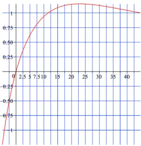
However, formal calculations (see Appendix) allowed us to plot the temporal growth rate 𝛾 [not to be confused with the loss coefficients 𝛾𝑒and 𝛾𝑎] of an acoustic perturbation as a function of 𝛼. A key result is that any such perturbation is initially unstable (𝛾 > 0) for any positive value of the acoustic dispersion, 𝛼 > 0, and even for some negative values (Fig. 7). The inertial regime may thus yield a full mirror behavior even for relatively small values of the acoustic dispersion.
5. Identification of regions of strong inertial dispersion
To identify the spectral regions of strong acoustic dispersion in which we may expect to observe the new inverted SBS mirror regime, as well as, conversely, the regions of weak dispersion where a bridge could be established between the two models, inertial and perturbative, we shall search the maximum values of the temporal growth rate of the acoustic amplitude, 𝛾, that is, the extrema of the function 𝛾 (𝑘, 𝛼).
To this end, and for the simplicity of the already bulky expressions, we will from now on shift to reduced variables, defining the reduced acoustic amplitude 𝐴𝑎 = 𝐸𝑎/|𝐸0𝑝|, the reduced acoustical losses 𝜇 = 𝛾𝑎/𝐾𝑆 𝐵 𝑆|𝐸0𝑝|, and setting:
Fig. 6. Same as Fig. 5: Successive zooms on the spatial evolution of the phases. Note the strong anticorrelation of the phases of the pump and Brillouin waves, yielding an almost uniform phase of the acoustic wave (Φ = 𝜙𝑝− 𝜙𝐵− 𝜙𝑎 ∼ 𝐶 𝑠𝑡)
Fig. 7. Temporal acoustic growth rate 𝛾 as a function of the acoustic dispersion 𝛼 for a set of values of the dissipation from 𝜇 = 20 to 𝜇 = 24.5, as obtained from the dispersion equation. Note that 𝛾 > 0 for any 𝛼 > 0.
𝑡/𝜏 = 𝑡𝐾𝑆 𝐵 𝑆|𝐸 0
𝑝| → 𝑡 𝑥/Λ0= 𝑥𝑛𝐾𝑆 𝐵 𝑆|𝐸 0
𝑝|/𝑐 → 𝑥 (7)
The linearized complex evolution equation for the acoustic amplitude now reads:
[𝜕𝑡+ 𝜀𝜕𝑥+ 𝜇 + 𝑖𝛼(𝜕𝑡 𝑡+ 2𝜇] (𝜕𝑡+ 𝜕𝑥) 𝐴𝑎= 𝐴𝑎 (8) Let us take:
𝜕𝑡−→ 𝛾 + 𝑖𝜔 𝜕𝑥−→ 𝑖𝑘 (9)
in order to obtain the complex characteristic equation:
giving rise to two real equations for the variables 𝛾, 𝜔, 𝑘 and 𝛼:
𝛾2− 𝜔2+ 𝜇𝛾 − 𝜔𝑘 − 𝜀𝜔𝑘 − 𝛼𝛾2𝜔+ 𝛼𝜔3− 𝛼𝛾2𝑘− 2𝛼𝜇𝜔 − 2𝛼𝜇𝑘 − 𝜀𝑘2− 2𝛼𝜔𝛾2+ 𝜀𝛾 𝑘 = 1 (11)
2𝜔𝛾 + 𝛾𝑘 + 𝜀𝑘 𝛾 + 𝜇𝜔 + 𝜇𝑘 + 𝛼𝛾3− 3𝛼𝜔2𝛾+ 2𝛼𝜇𝛾 − 2𝛼𝜔𝛾𝑘 = 0 (12) The aim is to eliminate 𝜔 from both equations to obtain an equation 𝛾 = 𝛾 (𝑘, 𝛼) and calculate 𝑀 𝑎𝑥[𝛾 (𝑘, 𝛼)] with respect to the parameter 𝛼. Ordering both equations in polynomial form with respect to 𝜔, we get:
𝛼𝜔3− 𝜔2− (𝑘 + 𝜀𝑘 + 3𝛼𝛾2+ 2𝛼𝜇) 𝜔 + 𝜇𝛾 − 𝛼𝛾2𝑘− 2𝛼𝜇𝑘 − 𝜀𝑘2+ 𝜀𝛾 𝑘 + 𝛾2 =1 (13)
− (3𝛼𝛾) 𝜔2+ (2𝛾 + 𝜇 − 2𝛼𝛾𝑘) 𝜔 + 𝛾𝑘 + 𝜀𝛾𝑘 + 𝜇𝑘 + 𝛼𝛾3+ 2𝛼𝜇𝛾) = 0 (14) These cubic Eq. (13) and quadratic Eq. (14) equations in 𝜔 can be solved, but the elimination of 𝜔 leads to a lenghty polynomial expression for 𝛾 = 𝛾 (𝑘, 𝛼) (detailed in the Appendix: Eq. (15)), which maximum with respect to 𝛼 can only be found numerically. Formal calculations using the Maple algorithm confirm that certain values of the acoustic (thus of the pump) frequency maximize the acoustic dispersion up to values where it can be considered strong.
Working Eq.(15) with Maple also allowed us to look into the dependence of the reduced dispersion 𝛼 over the wavevector 𝑘. For a given value 𝜇 of the losses, we obtain a double implicit mathematical solutions 𝛼(𝑘) of Eq. (15), as shown in Figure 8. Of these two, only the lower one presents a physical meaning. The apparent avoided crossing between the upper and the lower solutions defines a critical value of the wavevector, 𝑘𝑐𝑟 𝑖 𝑡
, below which the dispersion reaches very high values (almost vertical section in Fig. 8, yielding 𝑘𝑐𝑟 𝑖 𝑡
∼ 2.8 for 𝜇 = 21).
Moreover, since 𝜔 varies almost linearly with 𝑘 (Fig.9), we can also deduce a critical acoustic frequency 𝜔𝑐𝑟 𝑖 𝑡
𝑎 below which the dispersion may be strongly enhanced.
6. Conclusion
We have established that, for singular values of the pump wavelength associated to high values of the acoustic group velocity dispersion, which may be observed in photonic crystal fibers, this latter parameter can have a significant influence on the dynamics of SBS devices.
We have further established the possibility of a new SBS mirror regime with an inverted spatial acoustic profile, which may offer a high reflectance (∼ 100%) even for rather small pump intensities for some special frequencies at which the acoustic dispersion is strong enough, that may appear with a high spectral selectivity in PCFs of, possibly, in specially designed Brillouin microcavities.
We have also identified a new nonlinear self-stabilisation process of the phase of the acoustic wave, which may occur in the inverted mirror regime when the pump intensity is severely depleted and drops to very low values.
Further research will nevertheless be needed in order to validate the full 3-wave inertial model of stimulated Brillouin scattering for weak or moderate values of the acoustic dispersion and/or of the pump power and determine the respective validity domains of this inertial model and of the pertubative acoustic dispersion model.
Disclosures
Fig. 8. Implicit solutions 𝛼(𝑘) of the dispersion relation (Eq. 15) for 𝛾 = 0.35, 𝜀 = 10−5 and 𝜇 = 21. Note, on the upper left, the avoided crossing between the upper and lower solutions, only the latter having a physical meaning, and the almost vertical slope below 𝑘𝑐𝑟 𝑖 𝑡 ∼ 2.8.
Fig. 9. Quasi-linear dispersion relation 𝜔(𝑘) for 𝛾 = 0.2573, 𝛼 = 0.745, 𝜀 = 0 and a set of values of the dissipation from 𝜇 = 4 to 𝜇 = 20, allowing to deduce 𝜔𝑐𝑟 𝑖 𝑡
from 𝑘𝑐𝑟 𝑖 𝑡 .
7. Appendix: Resolution of the complex dispersion relation in the inertial limit
Eqs. (13) and (14) contain six variables, namely 𝜔, k, 𝜀 = 𝑐𝑎
𝑐, the reduced acoustic dispersion 𝛼 and losses 𝜇, and the growth rate 𝛾 of the acoustic instability.
We are interested on the function 𝛾 (𝛼) and we thus keep the other variables as known parameters. Eliminating 𝜔 and calculating the lexicographical Gröbner basis expression [58], we
obtain the following 5-parameter polynomial : 𝐸 =64 𝛾9𝛼4 − 3 𝛾7𝛼4𝑘2 − 8 𝛾5𝛼4𝑘4 + 192 𝛾7𝜇𝛼4 + 96 𝛾7𝜀𝛼3𝑘 + 18 𝛾6𝜀𝛼3𝑘2 − 68 𝛾5𝜇𝛼4𝑘2 − 34 𝛾5𝜀𝛼3𝑘3 + 8 𝛾4𝜀𝛼3𝑘4 − 16 𝛾3𝜇𝛼4𝑘4 − 8 𝛾3𝜀𝛼3𝑘5 + 144𝛾5𝜇2𝛼4 + 64 𝛾7𝛼3𝑘 + 60 𝛾6𝜇𝛼3𝑘 + 144𝛾5𝜇𝜀𝛼3𝑘 + 9 𝛾5𝜀2𝛼2𝑘2 + 108 𝛾4𝜇𝜀𝛼3𝑘2 − 124 𝛾3𝜇2𝛼4𝑘2 + 54 𝛾4𝜀2𝛼2𝑘3 + 4 𝛾5𝛼3𝑘3 − 10 𝛾4𝜇𝛼3𝑘3 − 124 𝛾3𝜇𝜀𝛼3𝑘3 − 31 𝛾3𝜀2𝛼2𝑘4 + 32 𝛾3𝜇3𝛼4 − 36 𝛾5𝜇𝜀𝛼2𝑘 + 116 𝛾5𝜇𝛼3𝑘 + 128 𝛾4𝜇2𝛼3𝑘 + 48 𝛾3𝜇2𝜀𝛼3𝑘 + 58 𝛾5𝜀𝛼2𝑘2 + 64 𝛾4𝜇𝜀𝛼2𝑘2 + 24 𝛾3𝜇𝜀2𝛼2𝑘2 + 4 𝛾3𝜀3𝛼 𝑘3 − 12 𝛾4𝜀𝛼2𝑘3 + 6 𝛾3𝜇𝜀𝛼2𝑘3 + 8 𝛾3𝜇𝛼3𝑘3 − 20 𝛾2𝜇2𝛼3𝑘3 + 4 𝛾3𝜀𝛼2𝑘4 − 10 𝛾2𝜇𝜀𝛼2𝑘4 + 32 𝛾7𝛼2 + 16 𝛾6𝜇𝛼2 − 12 𝛾5𝜇2𝛼2 + 36 𝛾4𝜇𝜀𝛼2𝑘 − 18 𝛾5𝛼3𝑘 − 24 𝛾3𝜇2𝛼3𝑘 + 16 𝛾2𝜇3𝛼3𝑘 + 18 𝛾4𝜀2𝛼 𝑘2 + 10 𝛾5𝛼2𝑘2 + 12 𝛾4𝜇𝛼2𝑘2 + 6 𝛾3𝜇2𝛼2𝑘2 − 24 𝛾3𝜇𝜀𝛼2𝑘2 + 16 𝛾2𝜇2𝜀𝛼2𝑘2 − 6 𝛾3𝜀2𝛼 𝑘3 + 4 𝛾2𝜇𝜀2𝛼 𝑘3 − 8 𝛾3𝛼3𝑘3 − 4 𝛾3𝛼2𝑘4 − 4 𝛾2𝜇𝛼2𝑘4 + 48 𝛾5𝜇𝛼2 + 32 𝛾4𝜇2𝛼2 − 8 𝛾3𝜇3𝛼2 + 24 𝛾5𝜀𝛼 𝑘 + 16 𝛾4𝜇𝜀𝛼 𝑘 − 4 𝛾3𝜇2𝜀𝛼 𝑘 + 54 𝛾4𝜀𝛼2𝑘 − 108 𝛾3𝜇𝛼3𝑘 + 18 𝛾4𝜀𝛼 𝑘2 + 12 𝛾3𝜇𝜀𝛼 𝑘2 − 3 𝛾2𝜇2𝜀𝛼 𝑘2 − 12 𝛾3𝜇𝛼2𝑘2 − 12 𝛾2𝜇2𝛼2𝑘2 + 8 𝛾 𝜇3𝛼2𝑘2 − 54 𝛾3𝜀𝛼2𝑘2 − 6 𝛾3𝜀𝛼 𝑘3 − 6 𝛾2𝜇𝜀𝛼 𝑘3 + 4 𝛾 𝜇2𝜀𝛼 𝑘3 + 36 𝛾4𝜇𝛼2 + 4 𝛾3𝜇2𝛼2 − 4 𝛾 𝜇4𝛼2 + 20 𝛾5𝛼 𝑘 + 32 𝛾4𝜇𝛼 𝑘 + 7 𝛾3𝜇2𝛼 𝑘 − 5 𝛾2𝜇3𝛼 𝑘 + 4 𝛾3𝜇𝜀𝛼 𝑘 − 4 𝛾 𝜇3𝜀𝛼 𝑘 + 𝛾3𝜀2𝑘2 − 𝛾 𝜇2𝜀2𝑘2 + 12 𝛾3𝛼2𝑘2 − 6 𝛾2𝜇𝛼2𝑘2 + 4 𝛾3𝛼 𝑘3 + 2 𝛾2𝜇𝛼 𝑘3 − 𝛾 𝜇2𝛼 𝑘3 + 𝜇3𝑎 𝑘3 − 36 𝛾3𝜇𝛼2 + 4 𝛾4𝜀 𝑘 − 3 𝛾2𝜇2𝜀 𝑘 − 𝛾 𝜇3𝜀 𝑘 − 4 𝛾3𝜇𝛼 𝑘 + 4 𝛾 𝜇3𝛼 𝑘 − 18 𝛾3𝜀𝛼 𝑘 − 2 𝛾3𝜀 𝑘2 + 2 𝛾 𝜇2𝜀 𝑘2 + 4 𝛾5 + 4 𝛾4𝜇 − 3 𝛾3𝜇2 − 4 𝛾2𝜇3 − 𝛾 𝜇4 − 27 𝛾3𝛼2 − 18 𝛾3𝛼 𝑘 − 12 𝛾2𝜇𝛼 𝑘 + 3 𝛾 𝜇2𝛼 𝑘 + 𝛾3𝑘2 − 𝛾 𝜇2𝑘2 − 4 𝛾3 + 3 𝛾 𝜇2 + 𝜇3 (15) From there, formal calculations in Maple allowed us to determine the growth rate 𝛾 as a function of 𝛼 for any given set of values of the other parameters (Fig. 7). These results appear mostly insensitive to the order of magnitude of the small parameter 𝜀, from 10−5to about 0.1.
It also allowed to plot the acoustic dispersion 𝑑2𝑘
𝑑 𝜔2 as a function of 𝜔𝑎 (Fig. 10) (Note that this physical parameter may vary with 𝜔𝑎 and 𝐼0𝑝 even as the reduced parameter 𝛼 = 𝑐𝑎 𝑑2𝑘 𝑑 𝜔2 𝐾𝑆 𝐵 𝑆 q 𝐼0𝑝/2𝜔𝑎remains constant.)
Figure 11 shows two sets of the same implicit mathematical solutions for different values of 𝜇. Note that these are not monotonous, almost parallel curves, as might appear at first glance, but two upper and two lower sets of solutions with avoided crossings, as emphasized by the zoom of Fig. 7.
References
1. J. Botineau, C. Leycuras, É. Picholle, and C. Montes, “Stabilization of a stimulated brillouin fiber ring laser by strong pump modulation,” J. Opt. Soc. Am. B 6, 300–312 (1989).
2. R. W. Boyd, K. Rzaewski, and P. Narum, “Noise initiation of stimulated brillouin scattering,” Phys. Rev. A 42, 5514 (1990).
3. C. Tang, “Saturation and spectral caracteristics of the stokes emission in the stimulated brillouin process,” J. Appl. Phys. 37, 2945 (1966).
4. R. Enns and I. Batra, “Saturation and depletion in stimulated light scattering,” Phys. Lett. 28A, 591–592 (1968). 5. S. Smith, F. Zarinetchi, and S. Ezekiel, “Narrow-linewidth stimulated brillouin fiber laser and applications,” Opt.
Lett. 16, 393–395 (1991).
6. É. Picholle, C. Montes, C. Leycuras, O. Legrand, and J. Botineau, “Observation of dissipative superluminous solitons in a brillouin fiber ring laser,” Phys. Rev. Lett. 66, 1454–1457 (1991).
Fig. 10. Acoustic dispersion curve 𝑑2𝑘
𝑑 𝜔2(𝜔) (numerical; 𝜇 = 17.5; 𝛼 = 0.8; 𝛾 = 0.29; and 𝜀 = 10−2). Note the strong maximum value of the dispersion (𝛽
𝑑 𝑦 𝑛 𝑎
𝑐𝑎
>1.55) for 𝜔𝑎=22.8.
Fig. 11. Same as Fig. 7 for different values of the losses (left to right : 𝜇 = 5 to 25 by increments of 2).The dots figure the avoided crossings, visible on the zoomed Fig. 7 but not resolved at this scale. Only the lower part of the curves have a physical meaning.
7. H. H. Diamandi and A. Zadok, “Ultra-narrowband integrated brillouin laser,” Nat. Photonics 13, 9–10 (2018). 8. S. Gundavarapu, G. M. Brodnik, M. Puckett, T. Huffman, D. Bose, R. Behunin, J. Wu, T. Qiu, C. Pinho, N. Chauhan,
J. Nohava, P. T. Rakich, K. D. Nelson, M. Salit, and D. J. Blumenthal, “Sub-hertz fundamental linewidth photonic integrated brillouin laser,” Nat. Photonics 13, 60–67 (2019).
9. C. Montes, A. Mamhoud, and É. Picholle, “Bifurcation in a cw-pumped brillouin fiber ring laser: coherent sbs soliton morphogenesis,” Phys. Rev. A 49, 1344 (1994).
10. C. Montes, D. Bahloul, I. Bongrand, J. Botineau, G. Cheval, A. Mamhoud, É. Picholle, and A. Picozzi, “Self-pulsing and bistability in cw-pumped brillouin fiber ring laser,” J. Opt. Soc. Am. B 16, 932–951 (1999).
11. D. J. Kaup, “The first-order perturbed stimulated brillouin scattering equations,” J. Nonlinear Sci. 3, 1427 (1993). 12. A. L. Gaeta and R. W. Boyd, “Stochastic dynamics of stimulated brillouin scattering in an optical fiber,” Phys. Rev. A
44, 3205–3209 (1991).
13. R. G. Harrison, J. S. Uppal, A. Johnstone, and J. V. Moloney, “Evidence of chaotic stimulated brillouin scattering in optical fibers,” Phys. Rev. Lett. 65, 167 (1990).
three-wave mixing and coherent stimulated scattering,” Phys. Rev. A 1992, 033847 (2015).
15. D. Boukhaoui, D. Mallek, A. Kellou, H. Leblond, F. Sanchez, T. Godin, and A. Hiddeur, “Influence of higher-order stimulated brillouin scattering on the occurrence of extreme events in self-pulsing fiber lasers,” Phys. Rev. A 100, 013809 (2019).
16. B. J. Eggleton, C. G. Poulton, P. T. Rakich, M. J. Steel, and G. Bahl, “Brillouin integrated photonics,” Nat. Photonics
13, 664–677 (2019).
17. R. I. Woodward, E. Kelleher, S. Popov, and J. Taylor, “Stimulated brillouin scattering of visible light in small-core photonic crystal fibers,” Opt. Lett. 39, 2330–2333 (2014).
18. K. H. Tow, Y. Léguillon, S. Fresnel, P. Besnard, L. Brilland, D. Méchin, D. Trégoat, J. Trolles, and P. Toupin, “Linewidth-narrowing and intensity noise reduction of the second order stokes component of a low threshold brillouin laser made of 𝑔𝑒10𝑎 𝑠22𝑠 𝑒68chalcogenide fiber,” Opt. Express 20, B104–B109 (2012).
19. H. H. Diamandi, Y. London, A. Bergman, G. Bashan, J. Madrigal, D. Barrera, S. Sales, , and A. Zadok, “Opto-mechanical interactions in multi-more optical fibers and their applications,” J. Sel. Top. Quantum Electron. 26, 2600113 (2020).
20. J.-C. Beugnot, S. Lebrun, G. Pauliat, H. Maillotte, V. Laude, and T. Sylvestre, “Brillouin light scattering from surface acoustic waves in a subwavelength diameter optical fiber,” Nat. Commun. 5 (2014).
21. A. Godet, A. Ndao, T. Sylvestre, V. Pecheur, S. Lebrun, G. Pauliat, J.-C. Beugnot, and K. P. Huy, “Brillouin spectroscopy of optical microfibers and nanofibers,” Optica 4, 1232–1238 (2017).
22. W. E. née Zhong, B. Stiller, D. Elser, B. Heim, C. Marquardt, and G. Leuchs, “Depolarized guided acoustic wave brillouin scattering in hollow-core photonic crystal fibers,” Opt. Express 23, 27707–27714 (2015).
23. F. Yang, F. Gyger, and L. Thévenaz, “Giant brillouin amplification in gas using hollow-core waveguides,” (2019). Preprint: arXiv:1911.04430v2.
24. N. T. Otterstrom, R. O. Behunin, E. A. Kittlaus, Z. Wang, and P. T. Rakich, “A silicon brillouin laser,” Science 360, 1113–1116 (2018).
25. R. Dehghannasiri, A. A. Eftekhar, and A. Adibi, “Raman-like stimulated brillouin scattering in phononic-crystal-assisted silicon-nitride waveguides,” Phys. Rev. A 96, 053836 (2017).
26. F. Gyger, J. Liu, F. Yang, J. He, A. S. Raja, R. N. Wang, S. A. Bhave, T. J. Kippenberg, and L. Th’evenaz, “Observation of stimulated brillouin scattering in silicon nitride integrated waveguides,” Phys. Rev. Lett. 124, 013902 (2020). 27. J. Zhang, O. Ortiz, X. L. Roux, É. Cassan, L. Vivien, D. Marris-Morini, D. Lanzillotti-Kimura, and C. Alonso-Ramos,
“Subwavelength engineering for brillouin gain optimization in silicon optomechanical waveguides,” Opt. Lett. 45, 3717–3720 (2020).
28. B. Morrison, A. Casas-Bedoya, G. Ren, K. Vu, Y. Liu, A. Zarifi, T. G. Nguyen, D.-Y. Choi, D. Marpaung, S. J. Madden, A. Mitchell, and B. J. Eggleton, “Compact brillouin devices through hybrid integration on silicon,” Optica
4, 847–854 (2017).
29. P. Dainese, P. S. J. Russell, G. S. Wiederhecker, N. Joly, H. L.Fragnito, V. Laude, and A. Khelif, “Raman-like light scattering from acoustic phonons in photonic crystal fiber,” Opt. Express 14, 4141–4150 (2006).
30. P. Dainese, P. S. J. Russell, N. Joly, J. Knight, G. S. Wiederhecker, H. L. Fragnito, V. Laude, and A. Khelif, “Stimulated brillouin scattering from multi-ghz guided acoustic phonons in nanostructured photonic crystal fibres guided acoustics,” Nat. Phys. 2, 388–392 (2006).
31. R. P. Moiseyenko and V. Laude, “Material loss influence on the complex band structure and group velocity in phononic crystals,” Phys. Rev. B 83, 064301 (2011).
32. J.-C. Beugnot and V. Laude, “Electrostriction and guidance of acoustic phonons in optical fibers,” Phys. Rev. B 86, 224304 (2012).
33. G. S. Wiederhecker, P. Dainese, and T. P. Mayer-Alegre, “Brillouin optomechanics in nanophotonic structures,” APL Photonics 4, 0711101 (2019).
34. G. Arregui, O. Ortiz, M. Esmann, C. M. Sotomayor-Torres, C. Gomez-Carbonell, O. Mauguin, B. Perrin, A. Lemaître, P. D. Garcia, and N. D. Lanzillotti-Kimura, “Coherent generation and detection of acoustic phonons in topological nanocavities,” APL Photonics 4, 030805 (2019).
35. G. P. Agrawal, Nonlinear Fiber Optics (Academic Press, 1989), 2nd ed. 36. R. W. Boyd, Nonlinear Optics (Academic Press, 2008), 3rd ed.
37. R. V. Laer, R. Baets, and D. V. Thourhout, “Unifying brillouin scattering and cavity optomechanics,” Phys. Rev. A
93, 053828 (2016).
38. C. Montes, “Efficient way to prevent reflection from stimulated brillouin backscattering,” Phys. Rev. Lett. 50, 1129–1132 (1983).
39. C. Montes, “Reflection limitation by driven stimulated brillouin rescattering and finite bandwidth spectral interaction,” Phys. Rev. A 31, 2366–2374 (1985).
40. J. Coste and C. Montes, “Asymptotic evolution of stimulated brillouin scattering: Implications for optical fibers,” Phys. Rev. A 34, 3940–3949 (1986).
41. C. Montes and J. Coste, “Optical turbulence in multiple stimulated brillouin backscattering,” Laser Part. Beams 5, 405–411 (1987).
42. J. Botineau, C. Leycuras, C. Montes, and É. Picholle, “A coherent approach to stationary stimulated brillouin fiber amplifiers,” Annales des Télécommunications 49, 479–489 (1994).
waveguides: Forces, scattering mechanisms, and coupled-mode analysis,” Phys. Rev. A 92, 013836 (2015). 44. V. Laude and J.-C. Beugnot, “Spontaneous brillouin scattering spectrum and coherent brillouin gain in optical fibers,”
Appl. Sci. 8, 907 (2018).
45. É. Picholle and A. Picozzi, “Guided-acoustic-wave resonances in the dynamics of a brillouin fiber ring laser,” Opt. Commun. 135, 327–330 (1997).
46. I. Bongrand, É. Picholle, and A. Picozzi, “Coherent model of cladding brillouin scattering in single-mode optical fibers,” Electron. Lett. 34, 1769 (1998).
47. I. Bongrand, É. Picholle, and C. Montes, “Coupled longitudinal and transverse stimulated brillouin scattering in single-mode optical fibers,” Eur. J. Phys. D 20, 121–127 (2002).
48. R. Engelbrecht, “Analysis of sbs gain shaping and threshold increase by arbitrary strain distributions,” J. Light. Technol. 32, 1689–1700 (2014).
49. M. Maldovan, “Sound and heat revolutions in phononics,” Nature 503, 209–217 (2013).
50. S. A. Nikitov, R. S. Popov, I. V. Lisenkov, and C. K. Kim, “Elastic wave propagation in a microstructured acoustic fiber,” IEEE transactions on ultrasonics, ferroelectrics, frequency control 55, 1831–1839 (2008).
51. V. Laude, J. M. Escalante, and A. Martinez, “Effect of loss on the dispersion relation of photonic and phononic crystals,” Phys. Rev. B 88, 224302 (2013).
52. S. D. Lim, H. C. Park, K. Lee, and B. Y. Kim, “High-accuracy measurement of cladding noncircularity based on phase velocity difference between acoustic polarization modes,” Opt. Express 18, 3574–3581 (2010).
53. R. I. Woodward, É. Picholle, and C. Montes, “Brillouin solitons and enhanced mirror in the presence of acoustic dispersion in a small-core photonic crystal fiber,” in Actes des 35𝑒
Journées Nationales d’Optique Guidée, Rennes, France,(https://hal.archives-ouvertes.fr/hal-01323737, 2015).
54. E. M. Dianov, A. Luchnikov, A. N. Pilipetskii, and A. Starodumov, “Electrostriction mechanism of soliton interaction in optical fibers,” Opt. Lett. 15, 314–316 (1990).
55. J. K. Jang, M. Erkintalo, S. G. Murdoc, and S. Coen, “Untraweak long-range interactions of solitons over galactical distances,” Nat. Photonics 7, 657–663 (2013).
56. C. Montes and A. Rubenchik, “Stimulated brillouin scatteringfrom trains of solitons in optical fibers: information degradation,” J. Opt. Soc. Am. B 9, 1857–1875 (1992).
57. C. Montes and R. Pellat, “Inertial response to nonstationary stimulated brillouin backscattering: Damage of optical and plasma fibers,” Phys. Rev. A 36, 2976–2979 (1987).