Markov chain Markov field dynamics: models and statistics

HAL Id: hal-00110370

https://hal.archives-ouvertes.fr/hal-00110370

Submitted on 5 Oct 2007

HAL is a multi-disciplinary open access

archive for the deposit and dissemination of sci-entific research documents, whether they are pub-lished or not. The documents may come from teaching and research institutions in France or

L’archive ouverte pluridisciplinaire HAL, est destinée au dépôt et à la diffusion de documents scientifiques de niveau recherche, publiés ou non, émanant des établissements d’enseignement et de recherche français ou étrangers, des laboratoires

Markov chain Markov field dynamics: models and

statistics

Xavier Guyon, Cécile Hardouin

To cite this version:

Xavier Guyon, Cécile Hardouin. Markov chain Markov field dynamics: models and statistics. Statistics A Journal of Theoretical and Applied Statistics, 2002, 36 (4), pp.339 - 363. �10.1080/02331880213192�. �hal-00110370�

Markov Chain Markov Field Dynamics: Models and Statistics X. GUYON and C. HARDOUIN

SAMOS - Université Paris 11

Abstract

This study deals with time dynamics of Markov fields defined on a finite set of sites with state space E, focussing on Markov Chain Markov Field (MCMF) evolution. Such a model is characterized by two families of potentials: the instantaneous interaction potentials, and the time delay potentials. Four models are specified: auto-exponential dynamics (E = R+), auto-normal dynamics (E = R), auto-Poissonian dynamics (E = N) and auto-logistic dynamics (E qualitative and finite). Sufficient conditions ensuring ergodicity and strong law of large numbers are given by using a Lyapunov criterion of stability, and the conditional pseudo-likelihood statistics are summarized. We discuss the identification procedure of the two Markovian graphs and look for validation tests using martingale central limit theorems. An application to meteorological data illustrates such a modelling.

Key words. Markov Field; Markov Chain dynamics; Auto-model; Lyapunov stability cri-terion; Martingale CLT theorem; Model diagnostic.

AMS Classification Numbers: 62M40, 62M05, 62E20.

1

Introduction

The purpose of this paper is to study time dynamics of Markov fields defined on a measurable state space E and a finite set of sites S. We present a semi causal parametric model called MCMF_{, Markov Chain of Markov Field, defined as follows: X = (X(t), t ∈ N}∗) is a Markov

1

e-mail: hardouin[guyon]@univ-paris1.fr Running head: Markov chain of Markov field

Mail address for correspondence: Cécile Hardouin, SAMOS, Université Paris 1, 90 rue de Tolbiac, 75634-Paris Cedex 13, France

chain on ES and X(t) = (Xi(t), i ∈ S) is a Markov field on ES conditionally to the past. We study the properties of this model characterized by two families of potentials: instantaneous interaction potentials and time-delay potentials.

Space time modelling has been considered in the literature by Preston (1974; [28]) for birth and death processes, Durrett (1995; [14]) for particles systems, Künsch (1984; [25]) and Koslov and Vasilyev (1980; [24]) for the study of reversible and synchronous dynamics, Pfeifer and Deutsch (1980; [26], [27]) for ARMA models in space. Among statistical studies and their appli-cations, some important contributions are those of Pfeifer and Deutsch (1980; [26], [27]), Besag (1974, 1977; [8], [9]), Keiding (1975; [23]) for birth and death process, Bennett and Haining (1985; [7]) for geographical data, Chadoeuf et al. (1992; [11]) for plant epidemiology. The as-ymptotic properties of these methods are obtained in a standard way (see Amemiya (1985; [1]), Dacunha-Castelle and Duflo (1986; [12]), Guyon (1995; [18]), Bayomog et al. (1994; [6]).

The aim of this paper is to specify the structure of conditional Gibbs models according to the kind of state space considered as well as to study ergodicity, identification, estimation and validation of such models. For simplicity, we consider only time homogeneous dynamics (but spatial stationarity is not assumed) and the one step Markovian property. Our results can be generalized to a larger dependency with respect to the past as well as to time inhomogeneous chains.

After the description of the probability transition P (x, y) of the model in Section 2, we study in Section 3 some properties about time reversibility, invariant probability measure, and marginal distributions and we show that the MCMF dynamics is equivalent to a time homogeneous space×time non causal Markov field representation.

Four examples are depicted in Section 4: the normal dynamics (E = R), the auto-exponential dynamics (E = R+), the Poissonian dynamics (E = N), and finally, the auto-discrete dynamics (E qualitative and finite). For each specification, we give sufficient conditions ensuring the ergodicity of the chain with the help of a Lyapunov criterion. Further, we specify the results for weak-reversible models, i.e. models such that the reverse (in time) transition Q(x, y) belongs to the same auto-model family as P (x, y).

estima-tion: consistency and asymptotic (in time) normality of the estimator, tests of nested hypotheses based on the CPL-ratio.

Section 6 is devoted to the identification problem i.e. to the determination of the dependency graphs G = {G, G−} related to the MCMF dynamics. Graph G is undirected and determines the instantaneous dependency, while graph G− is directed and associated to the time-delay dependency. In the Gaussian case, the characterization of G is given through the partial-autocorrelations; for non-Gaussian models, we suggest a stepwise procedure based on the CPL. In Section 7, we propose two validation tests based on CLT for martingales. We conclude this paper in Section 8 with the study of a real set of meteorological data to which we fit an auto-logistic MCMF model. The data consist of daily pluviometric measures on a network of 16 stations in the Mekong Delta (Vietnam) during a three-month period (Tang 1991; [31]). The auto-logistic model allows for information to be gathered on spatial and temporal dependencies, and the forecasting is relatively accurate for some sites. This study has to be considered as a first illustrative attempt; there is no doubt that it will have to be refined in a precise investigation and then compared to other space time models, like hidden Markov chains or threshold models. It will, of course, be interesting to take into account the dual feature of such data (it is not raining or the precipitation level is observed in R+∗) and integrate it in a Gibbs model. Such a generalization and comparisons to other models are subjected to another study actually in progress.

2

Notations and description of the MCMF model

Let S = {1, 2, ..., n} be a finite set of sites. We call X an MCMF model if X is a Markov Chain of Markov Fields (conditionally to the past). The latter are defined on a measurable state space (E, E) equipped with a positive σ-finite measure ν (ν is usually the counting measure if E is discrete, and the Lebesgue one if E ⊆ Rp). The product space is (Ω, O) = (ES, E⊗S) with the product measure νS _{= ν}⊗S_{. We shall consider the case Ω = E}S _{but all the following still holds}

for Ω = Π_i∈SEi, with measures νi on measurable spaces (Ei, Ei), i ∈ S.

We use the following notations. Let A be a subset of S; we denote xA = (xi, i ∈ A) and xA= (xj, j ∈ S \ A). Let G be a symmetric graph on S without loop: hi, ji denotes that i and

j are neighbours (in particular, i 6= j). The neighbourhood of A is ∂A = {j ∈ S : j /∈ A s.t. ∃ i ∈ A with hi, ji}. We shall write xi = x{i}_{and ∂i = ∂{i}. With these notations, our MCMF} model X is the following:

•X = (X(t), t ∈ N∗_{) is a homogeneous Markov chain on Ω,}

• • X(t) = (Xi(t), i ∈ S) is, conditionally to X(t − 1), a Markov field on S, with Xi(t) ∈ E. We suppose that the transition probability measure of X has a density P (x, y) w.r.t νS_.

If E is discrete, P (x, y) = P (X(t) = y|X(t − 1) = x). We look at models for which P (x, y) is defined by an (x) − a.s. admissible conditional energy U(y|x), i.e. such that

P (x, y) = Z−1_{(x) exp U (y|x) and Z(x) =} Z

Ωexp U (y|x)ν S

(dy) < ∞ (1)

(Z(x) =P_{Ωexp U (y|x) < ∞ if E is discrete). Let X(t − 1) = x. From the Moebius inversion} formula (Besag 1974, [8]; Prum 1986, [29]; Guyon 1995, [18]), there exists a minimal family Cx of non empty subsets of S, and conditional potentials Φ∗W(.|x) for each W ∈ Cx such that U (y|x) =PW ∈CxΦ

∗ W(y|x).

Throughout the paper, we suppose that Cx = C does not depend on x. If we denote 0 a reference state in Ω (0 is 0 when E = N, R or R+), then, almost surely in x, we can choose (in a unique way) potentials according to the “identifiability conditions”: Φ∗_{W(y|x) = 0 if for some} i ∈ W, yi= 0. Besides, for each W in C, there exists a family CW of non-empty parts of S such that the potential Φ∗_W can be written as:

Φ∗_{W(y|x) = Φ}W(y) + X W0_∈CW

ΦW0_,W(x, y)

This means that the energy U is linked to two families of potentials: instantaneous interaction potentials {ΦW, W ∈ C} and “conditional” interaction potentials {ΦW0,W, W ∈ C, W0 ∈ CW}. The semi-causal representation is associated to G = {G, G−} where G and G− are defined respectively by the instantaneous and time-delay dependencies:

hi, jiG⇔ h(t, i), (t, j)iG⇔ ∃W ∈ C s.t. {i, j} ⊆ W and ΦW 6= 0

hj, iiG− ⇔ h(t − 1, j), (t, i)iG⇔ ∃W ∈ C, W0 ∈ CW s.t. ΦW0,W 6= 0, i ∈ W, j ∈ W0 Note that G− is a directed graph while G is not. Let us define C− = ∪

W ∈CCW; then U (y|x) = P

Thus we finally write: P (x, y) = Z−1_{(x) exp{}X W ΦW(y) + X W1,W2 ΦW1,W2(x, y)} (2)

where we have put: P_W for P_{W ∈C} and P_W

1,W2 for P

W1∈C−,W2∈C, with ΦW(y) = 0 (resp. ΦW1,W2(x, y) = 0) if for some i ∈ W (resp. i ∈ W2), yi = 0.

There are three components in the neighbourhood of a site i: •∂i = {j ∈ S \ {i}, hi, jiG}: the t-instantaneous neighbourhood of i •∂i−= {j ∈ S, hj, iiG−}: the (t − 1)-antecedent neighbourhood of i •∂i+_{= {j ∈ S, hi, ji}

G−}: the (t + 1)-successor neighbourhood of i

The semi-causal representation is related to ∂i and ∂i−, while the non causal representation that we will present in the next section depends on ∂i, ∂i− and ∂i+.

Therefore, for each t ≥ 1 and A ⊂ S (A 6= ∅), the conditional distribution of XA(t) given the past and XA(t) = yA depends on X_∂A−(t − 1) = x∂A− and X∂A(t) = y∂A only, where ∂A−_{= {i ∈ S : ∃j ∈ A s.t. hi, jiG}−}. The corresponding conditional energy is:

UA(yA|yA, x) = X W :W ∩A6=∅ ΦW(y) + X W2:W2∩A6=∅ {X W1 ΦW1,W2(x, y)}

3

Some properties of an MCMF

3.1

Time reversibility, invariant and marginal distributions

In this section we only consider potentials ΦW1,W2 such that ΦW1,W2(x, y) = 0 if for an i ∈ W1, xi = 0 or for a j ∈ W2, yj = 0. When there is no ambiguity, 0 denotes also the layout with 0 in any site of S.

The transition P is synchronous if we can write P (x, y) =Q_s∈Sps(x, ys): the values at all sites s are independently and synchronously relaxed with distributions ps(x, .) in s.

Proposition 1 (i) The chain is time-reversible if and only if for all W1, W2, x, y : ΦW1,W2(x, y) = ΦW2,W1(y, x). In this case, P has an unique invariant probability measure given by:

π(y) = π(0)P (0, y)

P (y, 0)= π(0)Z

−1_{(0)Z(y) exp}X W

(ii) This invariant measure π is usually not a Markov field. If the transition P is syn-chronous and reversible, then π has a Markov property.

Proof:

(i) This can be derived from Künsch (1984), and Guyon (1995, Theorem 2.2.3.). (ii) We give in Appendix 1 two examples of non Markovian π.

If P is synchronous, only singletons occur for W in ΦW and for W2 in ΦW1,W2. As the chain is reversible, ΦW1,W2 ≡ 0 if either |W1| > 1 or |W2| > 1. This means that P (xi(t)|x

i_{(t), x(t − 1)) =} P (xi(t)|x∂i−(t − 1)), so that, P (x, y) = Z−1_{(x) exp{}X s∈S Φs(ys) + X hs0_,si G− Φ_{s0_},{s}(xs0, ys)} = Y s∈S ps(x, ys)

with ps(x, ys) = Z−1(x) exp{Φs(ys) +Ps0Φ_{s0_},{s}(xs0, ys)}. Then we have: π(y) = π(0)Z−1(0)Z(y)Y s∈S exp Φs(ys) Besides, if Us(zs, y) = Φs(zs) +P_s0_∈∂s−Φ_{s0_},{s}(ys0, zs), Z(y) = R exp{P_s∈SU (zs, y)}νS(dz) = Q s∈S R

exp U (zs, y)ν(dzs) = expP_s∈SΨ∂s−(y_∂s−) with Ψ_∂s−(y_∂s−) = ln{P_z

sexp U (zs, y)}.¤ Example 1 A synchronous and reversible transition.

Let E = {0, 1}, S is the one dimensional torus; the transition P (x, y) = Z−1(x) exp{αP_i∈Syi(xi−1 +xi+1)} is reversible with invariant law π(y) = π(0)Z−1(0) expP

i∈S

Φ_i−1,i+1(y), where Φ_i−1,i+1(y) = ln{1 + exp α(yi−1+ yi+1)}. The conditional distribution at site l depends on yl−2 and yl+2. Marginal distributions

For A ⊆ S, A 6= S, the marginal distributions (yA|x), conditionally to x, are generally not local in x, and not explicit and not local in y, except in specific cases as the Gaussian case. This is illustrated in Appendix 2.

3.2

Non causal Markov Field representation

Let X be an MCMF with the semi-causal representation (2). We are going to show that there is a unique equivalent time homogeneous space×time non-causal Markov field representation given

by the bilateral transitions: for X(t − 1) = x and X(t + 1) = z, P (y|x, z) = Z−1(x, z) exp{ X W1,W2 {ΦW1,W2(x, y) + ΦW1,W2(y, z)} + X W ΦW(y)} (3)

where the normalizing constant Z(x, z) is finite a.s in (x, z). The time translation invari-ant potentials on S = S × Z are eΦ_{W ×{0}}(y, 0) = ΦW(y) and eΦW1×{0},W2×{1}((x, 0), (y, 1)) = ΦW1,W2(x, y). The non-causal representation depends on all the three neighbourhoods ∂i, ∂i− and ∂i+_.

Proposition 2 The representation (2) of MCMF dynamics with the neighbourhood system {∂i, ∂i−_{, i ∈ S} is equivalent to the S Space×Time Markov-Field representation (3) with the} neighbourhood system {∂i, ∂i−, ∂i+_{, i ∈ S}.}

Proof:

(i) It is easy to see that the chain is also a two-nearest neighbours Markov field in time. Let τ be the density of X(0); the likelihood of (x(0), x(1), ...x(T )) is τ (x(0))Q_{t=1,TP (x(t − 1), x(t)).} For 1 ≤ t ≤ T − 1, the conditional density is:

P (x(t)|x(t − 1), x(t + 1)) = R P (x(t − 1), x(t)) P (x(t), x(t + 1)) ΩP (x(t − 1), a(t)) P (a(t), x(t + 1)) νS(da)

.

Let us denote x = x(t − 1), y = x(t), z = x(t + 1). As (X(t + 1) | X(t − 1) = x) admits an a.s. finite density, Z(x, z) = P (X(t + 1) = z | X(t − 1) = x) =RΩP (x, a) P (a, z) ν

S_{(da), is finite.} We obtain from (2): P (y|x, z) = expnP_W 1,W2{ΦW1,W2(x, y) + ΦW1,W2(y, z)} + P W{ΦW(y) + ΦW(z)} o R Ωexp nP W1,W2{ΦW1,W2(x, a) + ΦW1,W2(a, z)} + P W{ΦW(a) + ΦW(z)} o νS_(da)

This is nothing other than (3).

(ii) Conversely, let X be the space×time Markov field on S (3) with the neighbourhood system {∂i, ∂i−, ∂i+_{}. The field being time-homogeneous, a direct computation shows that its} semi-causal representation is (2). ¤

We can derive easily from (2) or (3) the semi-causal or non-causal conditional distributions at any point (i, t). Note that we have for each i, j : i ∈ ∂j−⇐⇒ j ∈ ∂i+.

Figure 1 shows an example of both representations. For the causal representation, we have ∂i = {j, k} , ∂i− = {i, j} (note that i ∈ ∂l−); while for the non-causal representation, ∂i = {j, k} , ∂i−= {i, j} , ∂i+= {i, j, l} and now i ∈ ∂l− and l ∈ ∂i+.

(include here Figure 1) The semi-causal conditional distribution at (i, t) is:

P (yi|y∂i, x∂i−) = Z_i−1(y∂i, x∂i−) exp{ X W1,W23 i ΦW1,W2(x, y) + X W 3 i ΦW(y)} (4)

The non-causal conditional distribution P (yi|y∂i, x∂i−, z∂i+) at (i, t) has conditional energy: X W1,W23i {ΦW1,W2(x, y) + ΦW1,W2(y, z)} + X W 3i ΦW(y)

A time inhomogeneous Markov field on S = S × T is not reducible to a semi-causal repre-sentation because ∂i− and ∂i+ are strongly related: the Markov field (3) is very specific. For the example considered in Figure 1, the non causal representation without the dotted arrow (i, t − 1) → (l, t) cannot be reducible to a causal representation. In all the following, we consider the time homogeneous framework.

Reversed dynamics

We give in Appendix 3 an example where the time reversed process of an MCMF is no more an MCMF.

4

Ergodicity of automodels

Here we examine several examples of auto-models (see Besag 1974; Guyon 1995), and we give conditions ensuring their ergodicity. We will use the Lyapunov Stability Criterion (see e.g. Duflo 1997; [13], 6.2.2). For n ≥ 0, let Fn= σ (X(s), s ≤ n) be the σ−algebra generated by the X(s), s ≤ n. The Lyapunov Stability Criterion is the following. Let us assume that a Markov chain defined on a closed subset of Rd is strongly Feller, and that there exists a Lyapounov function V such that, for n > 0, and for some 0 ≤ α < 1 and β < ∞

Then if there is at most one invariant probability measure, the chain is positive recurrent. Besides, the following law of large numbers applies: _n+11 P_k=0,nϕ(Xk)

a.s.

→ µ(ϕ) for any µ−integrable function ϕ, where µ is the invariant measure of the chain. A difficulty is to check whether ϕ is µ−integrable. Another useful result is available: we get the same law of large numbers for any function ϕ which is µ-a.s. continuous and s.t. |ϕ| ≤ aV + b for some constants a, b.

4.1

The autoexponential dynamics

Let us consider S = {1, 2, · · · , n}, and E = R+. We suppose that for each i, conditionally to ¡

Xi(t) = yi_{, X(t − 1) = x}¢(later, we shall note this condition (yi, x)), the distribution of Xi(t) is exponential with parameter λi(yi, x) (in fact λi(y∂i, x∂i−)). From Arnold and Strauss (1988; [3]) we can write: −U(y|x) =X i∈S αi(x)yi+ X W :|W |≥2 λW(x)yW

with yW = Q_i∈Wyi, αi(x) > 0 for any x and λW(x) ≥ 0. Then, the parameters are equal to λi(yi, x) = αi(x) +P_{W 3i}λW(x)yW \{i}. The ergodicity of the chain is obtained through the following assumption:

E1 (i) _{∀i ∈ S, ∀W , x → α}i(x) and x → λW(x) are continuous. (ii) _{∃a ∈ (0, ∞), s.t. ∀x ∈ (R}+)S_{, ∀i ∈ S : α}i(x) ≥ a.

Proposition 3 Under assumption E1, the autoexponential dynamics is positive recurrent. The strong law of large numbers holds for any integrable function and particularly for functions x 7→ f (x) such that |f(x)| ≤ αVr(x) + β (for some finite constants α and β) with Vr(x) =P_i∈Sxri, r being any positive integer.

Proof: The proof uses the Lyapounov stability criterion.

• The lower bound condition E1 (ii) says that exp U(y|x) ≤ exp −aP_i∈Syi, which is Lebesgue integrable. Then, the chain is strongly Feller.

• As P is strictly positive, the chain is irreducible and there exists no more than one invariant distribution (see Duflo (1997), Proposition 6.1.9).

• On the other hand, for any positive integer r, we have for all x, y ∈ E, i ∈ S, E£_{Xi(t)}r|x, yi ¤ = Γ(r + 1) λi(yi, x)r ≤ Γ(r + 1) ar It follows: E [Vr(X(t))|X(t − 1) = x] ≤ Γ(r + 1) ar |S| < ∞ (5)

where |S| is the cardinal of S. ¤

Example 2 A case of “weak-reversibility”

We assume that, conditionally to ¡Xi_{(t − 1) = x}i_{, X(t) = y}¢_{, the reversed transition Q(y, x)} is also exponential with parameter µ_i(xi, y). Then, from Arnold and Strauss (1988), the joint density for (X(t − 1) = x, X(t) = y) must be:

f (x, y) = C exp U (x, y), with U (x, y) = − X

W =W1×W2⊂S2,W 6=∅

λW xW1yW2

with λW > 0 if |W | = |W1| + |W2| = 1 and λW ≥ 0 if |W | ≥ 2. So E1 is satisfied. Example 3 Besag’s conditional auto-models

We consider the case of conditional auto-models, i.e. for W ⊆ S, λW = 0 if |W | > 2. Therefore:

−U(y|x) =X i∈S αi(x)yi+ X hi,ji β_ij(x)yiyj.

E1-(ii) is satisfied if αi(x) ≥ a and βij(x) ≥ 0 for all x, i, j. For example, if

−U(y|x) =X i∈S δiyi + X hi,jiG β_ijyiyj+ X hj,ii_G− αjixjyi (6)

with δi > 0, βij and αij ≥ 0, the distribution of Xi(t) conditionally to (yi, x) is exponential with parameter λi(yi, x) = δi+P_j∈∂iβijyj+P_l∈∂i−αlixl. The condition E1 is fulfilled .

4.2

The autonormal dynamics

Let E = R. We assume that the conditional distribution of Xi(t) given Xi(t) = yiand X(t−1) = x is Gaussian with mean µ_i(yi, x) and variance σ2_i(yi, x). The principle of compatibility requires (see Arnold and Press (1989; [2]), Arnold, Castillo and Sarabia (1991; [4])) that the conditional energy is of the following feature:

−U(y|x) =X i∈S {αi(x)yi+ βi(x)y2i} + X W s.t. |W |≥2 γ_W(x)ylW W where ylW W = Q i∈Wy li

i , li = 1, 2, and the functions α, β, γ ensuring that all the conditional variances are positive and U (.|x) is admissible.

Let us consider now Besag’s automodels. Then −U(y|x) = −P_i∈S{αi(x)yi+ βi(x)yi2} + P

hi,jiG{γij(x)yiyj + δij(x)y 2

iyj+ νij(x)yiyj2+ χij(x)y2iy2j}. A typical example is: P (x, y) = Z−1_{(x) exp −{}X i∈S yi(δi+ P l∈∂i− αlixl+ γiyi) + P hi,ji β_ijyiyj} (7) with γ_i > 0, β_ij = β_ji such that the matrix Q = (Qij) defined by Qii = 2γi and Qij = βij

is definite positive. The conditional distribution of Xi(t) given (yi, x) is Gaussian with mean −(δi+P_l∈∂i−αlixl+P_j∈∂iβijyj)/2γi and variance (2γi)−1.

Ergodicity: We consider the model (7). Let us note ∆ = (∆il), ∆il = −αli, i, l ∈ S, and δ = (δi); a direct identification of the distribution of (Y | x)= (X(t) | X(t − 1) = x) gives.

(Y | x) ∼ NS(m + Ax, Γ), with m = −Q−1δ, A = Q−1∆, and Γ = Q−1.

This can be written as an AR(1) process X(t) = m + AX(t − 1) + ε(t) with a Gaussian white noise ε having covariance matrix Γ. Define τ =(I − A)−1m when (I − A) is regular. Then the zero-mean variable X∗_{(t) = X(t) − τ verifies X}∗(t) = AX∗_{(t − 1) + ε(t). Let ρ(A) be the} spectral radius of A (i.e. the greatest modulus of its eigen values).

Proposition 4 _{If ρ(A) < 1, then (I − A) is regular and the chain is ergodic with a Gaussian} stationary measure µ.

Proof: The result is classic, given for example in Duflo (1997), Theorem 2.3.18. As ε is Gaussian, the stationary distribution for X∗ is the one ofP_k≥0Ak_{ε(k), i.e. N}S(0, Σ), Σ being

the unique solution of Γ = Σ − AΣ(tA), that is Σ = P_k≥0AkΓ(tA)k. For X(t), we add the mean τ . As ε has finite moments of all orders, we get the strong law of large numbers for any continuous integrable function. ¤

4.3

The Auto-Poissonian dynamics

Now E = N (ν is the counting measure) and we consider the dynamics associated with the following conditional energy:

U (y|x) =X i∈S

{αi(x)yi− ln(yi!)} +P i6=j

β_ij(x)yiyj

where β_{ij(x) ≤ 0 for all i, j in order to make U admissible. Conditionally to (y}i, x), Xi(t) has a Poisson distribution with parameter λi(yi, x) = exp{αi(x) + P

j:j6=i

β_ij(x)yj}. The ergodicity of the chain is obtained through the following hypothesis:

P1: _{∃ M < ∞ such that ∀i ∈ S, supx}αi(x) ≤ M

Proposition 5 Under P1, the auto-Poissonian chain is positive recurrent. Besides, the strong law of large numbers holds for any µ-integrable function and for any functions f such that |f(x)| ≤ αGu(x) + β (for some finite constants α and β) where Gu(x) = Q_i∈Seuixi , for any fixed u ∈ (R+)S.

Proof: The proof follows the same lines as the one given for the auto-exponential dynamics. P1 implies that λi(yi, x) ≤ eM. Then the transition is strongly Feller. As this transition is strictly positive, the invariant measure is unique.

For the conditional moment generating function, we have, for all s > 0, ΨXi(s) = E

£

esXi(t)_|yi_{, x}¤_{= e}λi(yi,x)(es−1) _{≤ exp(e}M_(es_{−1)). Let us set u = (u}

i, i ∈ S) ∈ (R+)S, Ku= max i∈S exp(eM(eui− 1)) and Gu(x) =Q_i∈Seuixi . Then, conditionally to X(t − 1) = x,

E [Gu(X(t))|x] = E   Y i∈S\{j} euiXi(t)_E h eujXj(t) |yj, x i |x   ≤ KuE   Y i∈S\{j} euiXi(t) |x   Taking successive conditional expectations, one obtains:

E " Y i∈S euiXi(t) | X(t − 1) # ≤ Ku|S|< ∞. ¤

For example, P1 is satisfied for

αi(x) = δi+ P l∈∂i−

αlixl and βij(x) = βij = βji (8)

with αli≤ 0 for any i, l, and βij < 0 if hi, ji and 0 else.

4.4

The auto-discrete dynamics

Let E be a finite qualitative set. The conditional energy of the auto-model is: U (y|x) =X

i∈S

αi(yi, x) + P hi,ji

β_ij(yi, yj, x).

As αi(.) and βij(.) are finite conditional potentials, the ergodicity is ensured without any

re-strictions on the parameters. For instance, the autologistic dynamics is defined for E = {0, 1}, and U (y|x) =P_i∈Sαi(x)yi+P_hi,jiβijyiyj; Xi(t) has a conditional Bernouilli distribution with parameter pi(yi, x) = exp δi(yi, x) 1 + exp δi(yi, x) with δi(yi, x) = αi(x) + X j∈∂i β_ijyj. (9)

For E = {0, 1, .., m}, the autobinomial dynamics is given by U(y|x)=P_i∈Sαi(x)yi+P_hi,jiβijyiyj. Conditionally to (yi, x), Xi(t) has a Binomial distribution B(m, θi(yi, x)) with parameter θi(yi, x) = (1 + exp{αi(x) + P_j∈∂iβijyj})−1 if we take the counting measure with density (m_yi) as reference measure.

5

Conditional Pseudo-Likelihood Statistics

5.1

Parametric estimation

We suppose that the transition probabilities of the MCMF depend on an unknown parameter θ, θ lying in the interior of Θ, a compact subset of Rd. When ergodicity holds, we can obtain the asymptotic properties of the estimators derived from the classic estimation methods (max-imum likelihood, pseudo max(max-imum likelihood, max(max-imum of another “nice” objective function) in a standard way. An analytical and numerical difficulty inherent to the maximum likelihood procedure is the complexity of the normalizing constant Zθ(x) in the likelihood; one can use

stochastic gradient algorithms to solve the problem (see Younes (1988), [33]); another numeri-cal option is to compute the log likelihood and its gradient by simulations via a Monte Carlo algorithm (see [16] Chapter 3 and [17]). A third alternative (see Besag (1974)) is to consider the Conditional Pseudo-Likelihood (CPL); in the presence of strong spatial autocorrelation this method performs poorly, and we then have to use the previous procedures. In the absence of strong dependency, it has good asymptotic properties, the same rate of convergence as the maximum likelihood estimator with a limited loss in efficiency (see Besag 1977 [10], Guyon 1995 [18], Guyon and Künsch 1992 [20]). The asymptotic behaviour follows in a standard way (see Amemiya (1985) and Dacunha-Castelle and Duflo (1986) for general theory; Besag (1984,[10]), Guyon and Hardouin (1992; [19]), Guyon (1995) for Markov field estimation; Bayomog (1994; [5]), and Bayomog et al. (1996) for field dynamics estimation). We briefly recall the main results. We assume that the chain is homogeneous and that for all i ∈ S, x, y ∈ E, θ ∈ Θ, the conditional distribution of Xi(t) given Xi(t) = yi and X(t −1) = x is absolutely continuous with respect to ν, with positive conditional density fi(yi, yi, x; θ) (which is in fact fi(yi, y∂i, x∂i−; θ)).

Let θ0 be the true value of the parameter, and P0 be the associated transition. The process is observed at times t = 0, · · · , T . Let us denote ˆθT = arg min

θ∈ΘUT(θ) the conditional pseudo-conditional likelihood estimator (CPLE) of θ, a value minimizing the opposite of the Log-CPL:

UT(θ) = − 1 T T P t=1 P i∈S ln fi(xi(t), xi(t), x(t − 1); θ)

The following conditions C and N ensure the consistency and the asymptotic normality of ˆθT

respectively.

Conditions for consistency (C):

C1: For θ = θ0, the chain X is ergodic with a unique stationary measure µ0. C2: _{(i) For all i ∈ S, x, y ∈ E, θ 7→ f}i(yi, yi, x; θ) is continuous..

(ii) There exists a measurable µ_{0 ⊗ P}0-integrable function h on E × E such that for all i ∈ S, θ ∈ Θ, x, y ∈ E, | ln fi(yi, yi, x; θ) − ln fi(yi, yi, x; θ0)| ≤ h(y, x).

C3: Identifiability: if θ 6= θ0 thenP_i∈Sµ0({x s.t. fi(., ., x; θ0) 6= fi(., ., x; θ) }) > 0.

Let f_i(1)(θ) and f_i(2)(θ) stand for the gradient and the Hessian matrix of fi(yi, yi, x; θ) with respect to θ. We define the following conditional (pseudo) information matrices: for x, y ∈ E, i, j ∈ S, i 6= j, θ ∈ V0, a neighbourhood of θ0, V0 ⊂ Θ:

Iij(y{i,j}, x, θ) = Eθ0[ f_i(1)(θ)f_j(1)(θ)0 fi(θ)fj(θ) | X {i,j}_{(t) = y}{i,j}_{, X(t − 1) = x],} Iij(x, θ) = Eθ0 £ Iij(X{i,j}(t), X(t − 1), θ) | X(t − 1) = x ¤ .

If Zi = _∂θ∂ ln fi(Xi(t), Xi(t), X(t − 1); θ)|θ=θ0, then Iij(y{i,j}, x, θ) is the covariance matrix of (Zi, Zj) given X{i,j}= y{i,j} and X(t − 1) = x.

Conditions for asymptotic normality (N): N1: For some V0 ⊂

◦

Θ, a neighbourhood of θ0, θ 7→ fi(yi, yi, x; θ) is two times continuously differentiable on V0 and there exists a measurable, µ0 ⊗ P0-square integrable function H on E × E such that for all θ ∈ V0, x, y ∈ E, 1 ≤ u, v ≤ d :

|_f1 i ∂ ∂θu fi(yi, yi, x; θ)| and | 1 fi ∂2 ∂θu∂θv fi(yi, yi, x; θ)| ≤ H(y, x) N2: I0= P i∈S Eµ0[Iii(X(t − 1), θ0)] and J0= P i,j∈S

Eµ0[Iij(X(t − 1), θ0)] are positive definite. Proposition 6 (Bayomog et al. (1996), Guyon and Hardouin (1992), Guyon (1995))

(i) Under assumptions C, ˆθT P0 −→ T →∞θ0

(ii) Under assumptions C and N, √T (ˆθT − θ0) −→D

T →∞Nd(0, I0 −1_J

0I0−1)

Identifiability of the model and regularity of I0: We give here sufficient conditions ensuring both (C3) and the regularity of the matrix I0. We suppose that each conditional density belongs

to an exponential family

fi(yi, yi, x; θ) = Ki(yi) exp{tθgi(yi, yi, x) − Ψi(θ, yi, x)}, (10) and set the hypotheses:

(H) : there exists (i(k), x(k), y(k), k = 1, d) s.t. g = (g1, g2, · · · , gd) is of rank d, where we denote gk= gi(k)(yi(k)(k), yi(k)(k), x(k)). We strengthen (H) in (H’):

(H’1) : _{for each i ∈ S, g}i(yi, yi, x) = hi(yi)Gi(yi, x) with hi(.) ∈ R (H’2) : _{∃a > 0 s.t. for each i, x, y}i_{, V ar{h}i(Yi) | yi, x)} ≥ a > 0

(H’3) : _{∃{(i(k), x(k), y}i(k)_{(k)), k = 1, d} s.t. G = (G}1, G2, · · · , Gd) is of rank d where Gk= Gk(yi(k)(k), x(k)). Obviously, (H’) implies (H).

Proposition 7 _{We suppose that the conditional densities {f}i(., yi, x; θ), i ∈ S} belong to the exponential family (10).

(i) Under (H), the model related to this family of conditional densities is identifiable. (ii) I0 is regular under (H’).

The proof is given in Appendix 4. A sufficient condition ensuring that J0 is positive definite can also be obtained using a strong coding set; this idea is developed in Jensen and Künsch (1994; [22]). It is sketched in the same Appendix 4. Many models fulfil (H) or (H’), for instance log-linear models or automodels. We give explicit conditions (C) and (N) for the autoexponential dynamics in section 5.3.

5.2

Testing submodels

It is now possible to test the submodel (Hq) : θ = ϕ(α), α ∈ Rq, q < d, ϕ : Rq → Rd such that:

• ϕ is twice continuously differentiable in a bounded open set Λ of Rq, with ϕ(Λ) ⊂ Θ, and there exists α0 ∈ Λ such that ϕ(α0) = θ0.

• • R = ∂ϕ∂α |α=α0 is of rank q.

Let ¯θT = arg minα∈ΛUT(ϕ(α)) be the CPLE of θ under (Hq), and I0 = I(α0) the associated information matrix I. If A is a positive definite matrix, with spectral decomposition A = P DP0_,

P orthogonal, we take A12 = P D 1

2P0 as a square root of A.

Proposition 8 CPL ratio test (Bayomog (1994), Bayomog et al. (1996), Guyon(1995)) If UT(θ) and UT(ϕ(α)) satisfy assumptions C and N, then, under (Hq), we have as T → ∞:

∆T = 2T ³ UT(¯θT) − UT(ˆθT) ´ _D −→ d−q_P i=1 λiχ21,i

where the χ2_1,i’s are independent χ2₁ variables and the λi, i = 1, d − q, are the (d − q) strictly positive eigenvalues of Γ0 = J01/2

£

I₀−1_{− R ¯}I₀−1R0¤J₀1/2.

Let C be a coding subset of S, i.e., for all i, j ∈ C, i 6= j, i and j are not (instantaneous) neighbour sites. We can define coding estimators as previously, but in the definition of the coding contrast U_TC_{(θ), the summation in i is then restricted to C. For those estimators, we}

have I₀C = J₀C; so the asymptotic variance for √T³bθC_{T − θ}0 ´

is (I₀C)−1, and the former statistic

has a χ2_d−q asymptotic distribution.

5.3

An example: The autoexponential model

Here we look at these various conditions for the model given in section 4.1. The assumption E1 ensures the ergodicity. For a positive integer r and Vr(x) = P_i∈Sxri, we define the following property for a function f :

There exist two finite constants α and β such that

f (x) ≤ αVr(x) + β (11)

We add the following hypotheses to obtain the consistency and the asymptotic normality of the CPL estimator.

E2_{For all i ∈ S, W ∈ C, θ ∈ Θ and x ∈ E, α}i(x, θ) and λW(x, θ) satisfy (11).

E3 _{If θ 6= θ}0, then there exists A ⊆ (R+)S, λ(A) > 0, such that for one i ∈ S and all x ∈ A, λ¡©y ∈ E | λi(yi, x, θ) 6= λi(yi, x, θ0)

ª¢ > 0

E4 _{The functions θ → α}i(x, θ), θ → λW(x, θ) are twice continuously differentiable for all x, i, j, W , and for all 1 ≤ u, v ≤ d, and the absolute values of their first and second order derivatives satisfy (11).

E5 I0 and J0 are positive definite.

E6 (H’) is satisfied and J0 is positive definite.

Proposition 9 Let bθT be the CPLE of θ for the autoexponential model. Then:

(i) under assumptions E1, E2, and E3, bθT is consistent. If we add E4 and E5, bθT is

asymptotically normal.

(ii) under assumptions E1, E2, E4 and E6, bθT is asymptotically normal.

Proof: E1 implies C1 and E4 implies C2-(i). E3 implies C3. Then we just have to show that E2 implies C2-(ii). The conditional density of Xi(t) is given here by ln fi(yi, yi, x; θ) = ln λi(yi, x; θ)−yiλi(yi, x; θ). Then ¯ ¯ln fi(yi, yi, x; θ)−ln fi(yi, yi, x; θ0) ¯ ¯≤¯¯¯ln λi(yi,x;θ) λi(yi,x;θ0) ¯ ¯ ¯+yi ¯ ¯λi(yi, x; θ)−λ

As ¯ ¯ ¯lnxy ¯ ¯

¯ ≤ |x − y| (x−1_{+ y}−1_{) for all x, y > 0, we obtain}¯¯ln f_{i(yi, y}i_{, x; θ) − ln f}

i(yi, yi, x; θ0) ¯ ¯ ≤ (2_a + yi) ¯ ¯λi(yi, x; θ) − λi(yi, x; θ0) ¯

¯ . Finally, there exist two integers r and r0 _{and four} con-stants a1, a2, a3, a4 such that we can take h(y, x) =P_i∈S2(2_a+ yi){a1Vr(x) + a2+ (a3Vr0(x) + a4)P_j6=iyj}.

On the other hand, E4 implies that the modulus of the first and second derivatives of λi(yi, x; θ) with respect to θ are bounded by a square integrable function of x and y, and this ensures N1. Finally, E5 is N2. In another hand, E6 ensures E3 and E5 (see Proposition

7). ¤

Example 4 The conditional-exponential dynamics.

For the particular model (6), all conditions E are fulfilled without any assumption on the parameters. Besides, E6 is satisfied with d = n + 1₂P_{i∈S|∂i| +}P_i∈S|∂i−_{|, λ}i(yi, x, θ) = t_θg

i(yi, x),tθ = t ³

(δi)i∈S, (βij)hi,jiG, (αji)hj,iiG− ´

∈ Rd_.

6

Model identification

We suppose that we want to fit a semi-causal MCMF dynamics model; first, we have to de-termine the graphs G and G−; then, we will estimate the parameters, and lastly validate the model. There are two possible strategies for the identification procedure, the choice depending on the complexity of the problem and on the number of sites. The first one is global : we could try to determine globally the graphs by CPL maximization, joined with a convenient “AIC” penalization criterion.

On the other hand, a less expensive procedure is to work locally site by site, providing estimations for ∂i and ∂i− _{for each site i ∈ S. For this, we maximize the likelihood of X}i(t), t = 1, T, conditionally to Xi_{(t) = y}i _{(|S| − 1 sites) and X(t − 1) = x (|S| sites) (the conditional} distribution of Xi(t) depends on (2|S| − 1) sites) using a backward procedure; we choose a small signification level for the adequate statistics in order to keep only the most significant variables. This can be associated with a forward procedure if we want to take into account a particular information on the geometry of S. Further, we have to harmonize the instantaneous neighbourhood relation to get a symmetric graph G: if j ∈ b∂i, we decide i ∈ c∂j. Thus we

generally get an overfitted model, and the next step is to reduce it by progressive elimination using a descending stepwise procedure. Finally, if we have got two or more models, we choose the one which minimizes the AIC (or BIC) criterion.

In a Gaussian context, the computation is particularly easy and fast, because it is linear and explicit. Using the partial correlation ρ_P, we have the characterizations (see Garber (1981; [15]); Guyon (1995), §1.4.): ρ_P(Xj , Xi|XLi) = 0 ⇐⇒ j /∈ Li = ∂i ∪ ∂i−. This equation allows us to determine Li by a fast linear stepwise procedure of the regression of Xi(t) on the (2|S| − 1) other variables.

For other log linear models, the conditional log likelihood is concave so we can get the CPLE using a gradient algorithm. We then consider the general procedure given previously. An alternative is to follow the Gaussian approach, even if the model is not Gaussian. This can be done when the dimension of the parameter becomes large enough to make the results suspicious and slow progressing. This procedure is used in section 8.

7

Model validation

7.1

Some Central Limit Theorems

In the case E ⊆ R, validation tests are based on the estimated conditional residuals. Let us denote θ0and bθT the true value of the parameter and its CPLE respectively. Let us set:

εit= Xi(t) − µit and bεit= Xi(t) − bµit (12) where µ_it(θ) = E[Xi(t)|Xi(t), X(t − 1); θ], µit = µit(θ0). bµit = µit(bθT) is explicit in y∂i, x∂i−, and bθT.

For an autodiscrete dynamics on a K-states space E, we will have an expression equivalent to (12), but with the (K − 1)-dimensional encoded variable Zi(t) related to Xi(t) (see section 7.2.4).

From (12), we propose a validation statistic; we derive its limit distribution using a Central Limit Theorem for martingales (Duflo (1997), Hall and Heyde (1980; [21])).

The latter allows for the detection of possible variance deviation. Anyway, those tests are more useful to reject a model than to select the best one.

7.1.1 CLT for the residuals εit

We denote A ⊥ B if the variables A and B are independent. Let C be a coding subset of S (for G), eit = _σ(εεit_it) and eet=P_i∈Ceit:

(i) eit is zero mean and of variance 1;

(ii) εit⊥ Xj(t) if i 6= j and εit ⊥ Xj(t − 1) for all j ∈ S.

Besides, for all i and j which are not neighbour sites, Xi(t) and Xj(t) are independent, conditionally to the past and the neighbourhood values on ∂i, ∂j. Then eit ⊥ ejs if t 6= s, for all i, j ∈ S, and conditionally to X(t − 1) and X_C(t), eit ⊥ ejt for all i, j ∈ C, i 6= j;

(iii) as E [eit|Ft−1] = E £ E£eit | yi, x ¤ Ft−1 ¤

= 0, (eit)t≥0 is a square integrable martingale

difference sequence w.r.t. the filtration (Ft= σ(X(s), s ≤ t), t ≥ 0). Then eet =P_i∈Ceit is also a square integrable martingale difference sequence.

We can thus apply a martingale’s CLT (Duflo (1996), Corollary 2.1.10). For a square inte-grable martingale (Mt), let (hMit) be its increasing process defined by:

hMit= hMit−1+ E[||Mt− Mt−1||2|Ft−1] for t ≥ 1, and hMi0 = 0. The first condition to check is:

hMiT T

P −→

T →∞Γ, for some positive Γ. (13)

We set Ms= s P t=1ee t; we then have: hMit− hMit−1= X i∈C E£e2_it|Ft−1¤=X i∈C E£E£e2_it|yi, x¤_|Ft−1¤_{= |C|} The second condition is the Lindeberg condition. It is implied by the following one:

∃ α > 2 such that E [|eet|α|Ft−1] is bounded (14) Therefore, (13) is fulfilled with Γ = |C|,whatever the model, while (14) has to be checked in each particular case.

Proposition 10 (Duflo (1997), Hall and Heyde (1980))

Let εit be defined by (12), C a coding subset such that eet fulfills (14). Then, 1 p |C|T T X t=1 eet −→D T →∞N (0, 1) 7.1.2 CLT for the squared residuals

Let us define wit = e2 it− 1 σ(e2 it) (15) The wit’s have the same properties of independency as the eit’s. Hence (wit) is a martingale difference sequence in t, and so isw_et=P_i∈Cwit, for C a coding subset of S. Let NT =Pt=1,Twet. As hNit− hNit−1 = Pi∈CE

£

w2_it|Ft−1¤ _{= |C|, the first condition (13) for the CLT is fulfilled.} The second condition will be ensured under:

∃ α > 2 such that E [| ewt|α|Ft−1] is bounded (16) Proposition 11 _{Let C be a coding subset of S , w}it be defined by (15) s.t. wet fulfills (16). Then,√1 |C|T P i∈C T P t=1 wit −→D T →∞N (0, 1)

As we do not know θ0, we apply the previous results to the residuals calculated with bθT. When CPLE is convergent, standard manipulations show that Propositions 10 and 11 still remain valid for the estimated residuals.

7.2

Applications

We give the explicit results for the auto-models studied in section 4. The proofs of the conditions (14) or (16) are given in Appendix 5.

7.2.1 The autoexponential dynamics

We suppose that we are in the framework of (6), assuming E1, E2, E3. Then bθT is convergent and we have: 1 p |C|T X i∈C T X t=1 beit −→D T →∞N (0, 1) and 1 2p_2|C|T X i∈C T X t=1 (_be2_{it− 1) −→}D T →∞N (0, 1)

7.2.2 The autopoissonian dynamics

We consider the framework of (8) and we suppose that the CPLE bθT is consistent. Then for

λi = λi(Xi(t), X(t − 1)), γ2 = P_i∈CE[λi] and σ2 = P_i∈CE[λi(λi+ 1) ¡ λi2+ 5λi+ 1 ¢ ], we have: 1 √ T X i∈C T X t=1 bεit −→D T →∞N (0, γ 2_{) and} 1 √ T X i∈C T X t=1 ¡ bε2it− λi(yi, x) ¢ D −→ T →∞N (0, σ 2₎

7.2.3 The autologistic dynamics

For E={0, 1} , we consider the framework of (9) and we assume:

B1: For θ 6= θ0, ∃ x, y ∈ E s.t., for an i ∈ S, pi(yi, x, θ) 6= pi(yi, x, θ0). Under assumption B1, we have:

1 p |C|T X i∈C T X t=1 beit −→D T →∞N (0, 1) and 1 p |C|T X i∈C T X t=1 beit.sign(beit) −→D T →∞N (0, 1) 7.2.4 The autodiscrete dynamics

More generally, if E is qualitative, E = {a0, a1, · · · , aK−1}, we consider the encoded (K − 1)-dimensional variable Zit ∈ {0, 1}K−1 linked to the Xi(t) by:

Zitl= 1 if Xi(t) = al, Zitl= 0 elsewise, 1 ≤ l ≤ K − 1.

We suppose that the conditional energy is given by U (zt|zt−1) = P_i∈SP_l=1,K−1zitl(δi,l + P

k=1,K−1αi,lkz_i(t−1)k) +P_hi,jiP_l=1,K−1P_k=1,K−1βij,klzitlzjtk. We have: 1 p (K − 1)|C|T X i∈C T X t=1 ³ t_ε itC −1 it εit− (K − 1) ´ _D −→ T →∞N (0, 1) where Cit = (Cit)kl, 1 ≤ k, l ≤ K − 1, with (Cit)kk = pik(zti, zt−1)(1 − pik(zit, zt−1)), (Cit)kl = (Cit)lk= −pik(zti, zt−1)pil(zti, zt−1) if l 6= k, and pil(zit, zt−1) = exp yitl

1 +P_l=1,K−1exp zitlyitl

(17)

7.2.5 The autonormal dynamics

In the framework of (7), we suppose that the ergodicity condition is fulfilled. We have: 1 p |C|T X i∈C T X t=1 eit −→D T →∞N (0, 1) and X i∈C T X t=1 2γ_iε2_{it −→}D T →∞χ 2 |C|T and so, 1 2p_|C|T X i∈C T X t=1 ¡ 2γ_iε2_{it− 1}¢ _−→D T →∞N (0, 1)

A third result holds, which uses the joint distribution on S of all the residuals. The εit’s co-variances are Cov(εit, εjt) = _2γ1

i if i = j, = − β_ij

2γiγj if j ∈ ∂i, and 0 else. Let Cε be the n × n covariance matrix of εt= (εit, i ∈ S). ThenP_t=1,T tεtCε−1εt∼ χ2_nT and thus

1 √ nT T X t=1 t_ε tC −1 ε εt −→D T →∞N (0, 1)

Let bθT be a consistent estimator of θ0and bCεis the estimate of Cεobtained by replacing the

para-meters by their estimates. Then, the three statistics T1, T2, T3 defined below are asymptotically Gaussian N (0, 1) and can be used for validation tests of the model:

T1= √1 |C|T P i∈C T P t=1be it ; T2= 1 2√|C|T P i∈C T P t=1 ¡ 2_bγibε2_{it− 1}¢ ; T3 = √1_nT T P t=1 t_bε tCbε−1bεt

8

MCMF modelling of meteorological data

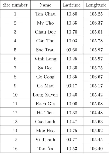
We have tried an MCMF modelling on a real set of meteorological data. The data comes from the study of Tang (1991) and consists of daily pluviometric measures on a network of 16 sites in the Mekong Delta (Vietnam). We have retained a period of 123 consecutive days from July to October 1983. Geographically, the 16 meteorological stations, situated at latitude 9.17 to 10.8 and longitude 104.48 to 106.67, are not regularly located (see table 1).

The data have been previously studied by Tang (1991); he proposed different models for each site, each being free of the other sites; this seems to be insufficient and hardly satisfactory.

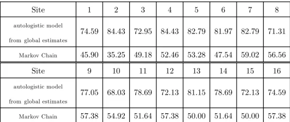
We study an MCMF autologistic model; we consider the binary {0,1} data where 1 stands for rain and 0 for no rain. The results lead to an average of exact prediction of about 77%,

which is rather satisfactory noting that the random part is large in this kind of meteorological phenomenon. We compare this model with a site-by-site Markov Chain, for which the prediction results are bad.

Of course, we do not pretend that our models are definitive and we know they need to be refined for effective forecasting. An interesting study would be to fit other competitive models of more or less the same dimension, as an Hidden Markov Chain (see e.g. .Zucchini and Guttorp 1991 [34], MacDonald and Zucchini 1997, [35]), the hidden states standing for the underlying climatic stage, or threshold models, the dynamics at the time t depending on the position of the state at the time t − 1 with respect to thresholds (see [32] and references herein). Also, these models should take into account the dual character of such a data, i.e. the binary feature {0} ∪ R+∗ of the space state. This is work in progress.

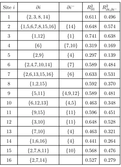
The first task is to identify the two dependency graphs. Considering the large number of parameters involved in the CPL procedure, we use the Gaussian linear procedure with the original data (see section 6); we fit a regression model on each site, with respect to the 15 other variables at the same time and all the 16 variables at the previous time. We then select the neighbours as the variables giving the best multiple correlation coefficient R2 _{in a stepwise}

procedure, taking into account the symmetry of the instantaneous graph together with a principle of parsimony. We give in table 2 the neighbourhoods and the R2 _{obtained from all the 31}

variables (denoted R2₃₁) and the R2 calculated on the selected neighbours (denoted R2_∂i,∂i−). The instantaneous graph has 25 links and the time-delay graph 17 links. We see that for each site, the instantaneous neighbourhood may contain few sites, while there are at most 3 sites making up the time delay neighbourhood. We note that if we draw the directed graph G− on a geographical map, there is a main direction of the arrows, which is roughly S-N.

(include here table 1 and table 2)

Going back to the binary data, we estimate the autologistic model (9): for each site i, Xi(t) has a Bernouilli distribution of parameter pi(t), conditionally to X∂i(t) and X∂i−(t), with pi(t) = (1 + exp −λi(t))−1 and λi(t) = δi+P_j∈∂iβijXj(t) +P_i∈∂i−αliXl(t − 1). The dimension of the model is 16+25+17=58. We first estimate the parameters site-by-site, maximizing the log

conditional pseudo-likelihoods; then, we calculate the validation statistics based on the square residuals (see section 7.2): Vi = √1_T PTt=1eˆit.sign(ˆeit) for each site i. Secondly, we proceed to the global estimation on the basis of the global pseudo-likelihood; we take as initial values the first site-by-site estimates for the parameters δi and αli, and the means of the two previous

estimations β_ij and β_ji (theoretically equal) for the instantaneous interaction parameters. We do not give here the results for the 58 parameters for sake of place, but we summarize the results: concerning the statistics Vi, each local model is accepted. The final (global) estimation provides results close to the individual ones. The validation statistic V = √1

CT P

i∈C PT

t=1ˆeitsign(ˆeit) computed for the coding set C = {3, 4, 5, 7, 8, 10, 11, 14} (of maximal size 8) is equal to −0.1186 and we do not reject the model.

Another way to validate the model is to compare the true data with what is predicted. So we compute the predicted values (maximizing the local conditional probabilities), first site by site (with the local estimates) and then globally (with the global estimates). Table 3 gives the percentages of similarity which spread out from 68.03% (site 10) to 84.43% (site 2), with a mean of 77.36% (for the global parameter’s estimate).

(include here table 3)

We compare our model with a site by site Markov chain. Of course, this alternative is very poor; as expected, the predictions are bad, spreading out between 35.25% and 59.02% with a mean equal to 51.84% (see Table 3). In conclusion, the autologistic model leads to a relatively correct forecasting; it could be better if we increase the number of links or the dependence in time, at the expense of the rising parametric dimension.

9

Appendices

9.1

Appendix 1: the invariant law

π of an MCMF is generally not Markovian

We illustrate this with two examples.

(1) The one dimensional marginal of a two dimensional Gaussian Markov field is not any-more a Markov process. Let us consider a centered Gaussian Markov isotropic field with respect

to the four-nearest neighbours over Z2 (see Besag, 1974 [10], Ripley, 1981 [30] and Guyon,1995 [18] §1.3.4.)

Xst= α(Xs−1,t+ Xs+1,t+ Xs,t−1+ Xs,t+1) + est, |α| < 1 4

with E[Xstes0t0] = 0 if (s, t) 6= (s0, t0). The spectral density of X is f (λ, µ) = σ2_e(1 − 2α(cos λ + cos µ))−1. The one index field (Xs,0, s ∈ Z) has spectral density

F (λ) = 2 Z π

0

f (λ, µ)dµ = 2πσ2_{e[(1 − 2α cos λ)}2_{− 4α}2]−12

which cannot be written _Q(e1iλ₎ or_{|P (e}1iλ_)|2 as for a Markovian or an AR process. The distribution π of (Xs,0, s ∈ Z) is not Markovian.

(2) Conditional Ising model : Ω = {0, 1}S, S = {1, 2, · · · , n} is the one dimensional torus with the agreement n + 1 ≡ 1, and P (x, y) = Z−1(x) exp{αP_i∈Sxiyi + βP_i∈Syiyi+1}. This chain is reversible and the invariant distribution can be written π(y) = CZ(y) exp{γP_i∈Syi+ βP_i∈Syiyi+1} where Z(y) is the normalizing constant of P (. | y). It is easy to see that log π(y) has a non zero potential ΦS on the whole set S.

9.2

Appendix 2: Two examples where marginals in y are not local in

x

(1) Binary state space. Let us consider a binary chain on the one dimensional torus S = {1, 2, · · · , n} (with n + 1 ≡ 1) with the transition

P (x, y) = Z−1_{(x) exp{α} n X i=1 xiyi+ β n X i=1 yiyi+1+ γ n X i=1 yi} Then Pi(yi|x) =PyiP (x, yi, yi) = eyi(αxi+γ)S yj ,j6=ieβyi(yj−1+yj+1)+Ai S yj ,j6=ieAi+e(αxi+γ) S yj ,j6=ieβ(yj−1+yj+1)+Ai , with Ai =

β P_j6=i,i−1 yjyj+1+ P_j6=i(αxj + γ)yj. This distribution depends on x on all sites. (2) A Gaussian example.

We take P (x, y) = Z−1_{(x) exp U (y|x) with U(y|x) = (y − m(x))}0_{Q(y − m(x)), where Q is} symmetric, definite positive, and E[Y |x] = m(x). For −U(y | x) =

n P i=1 (γ_iy2 i+δiyi)+ n P i=1 αixiyi+ n P i,j=1,<i,j> β_ijyiyj, m(x) = Q −1

2 (δ+αx) where δ = (δi)i∈S, αx = (αixi)i∈S, and V ar[Y |x] = 1 2Q−1: V (Y | x)−1_{= 2Q is local in x but it is easy to find parameters for which each component ml(x)} of m(x) depends on all xi, i ∈ S.

9.3

Appendix 3: An example of a reverse MCMF non MCMF

We consider S = {1, 2, · · · , n}, X = X(0), Y = X(1) and we suppose that Z = (X, Y ) is a 2n-dimensional centered Gaussian variable with covariance Σ =



 ∆ B

t_{B ∆} 

. Then, (Y | x) ∼ Nn(Ax, Q), where A = tB∆−1 and Q = ∆ − tB∆−1B. We fix ∆ and look at B as a parameter (s.t. Σ is definite positive).

If we want conditional independence for {(Xi(1) | X(0) = x), i = 1, n}, we force Q to be diagonal; this involves n(n−1)₂ conditions on B, for n2 degrees of freedom.

On the other hand, (X | y) ∼ Nn(T y, R) where T = B∆−1 and R = ∆ − B∆−1 tB. We can chose B such that for some i, Rij 6= 0 for any j. In such a case, (Xi(0) | xi, y) depends on xi on whole S\{i} and the reverse chain is not an MCMF.

For example, this happens for n = 2 if we take ∆ =   1 1 2 1 2 1  , B =   1 4 3 4 −12 0  .

9.4

Appendix 4: Parametric identifiability; regularity of

I

and

J

First we take ν∗S _{= ⊗i∈S}Kiν as the reference measure, where Ki is defined in (10).

Identifiability. We suppose that the conditional densities are equal for θ and θ0. Then, for each

i ∈ S, x and yi we have t

(θ − θ0)gi(yi, yi, x) = Ψ(θ, yi, x) − Ψ(θ0, yi, x)

But the right member is 0 as gi(0, yi, x) = 0. Identifiability follows because the d × d matrix g is regular.

Regularity of I0. First we note that for the stationary distribution

I0= E_X(t−1),Xi_(t)[ X i∈S V arXi(t){gi(Xi(t), X i (t), X(t − 1))}]. Then, under (H’), we have

X i∈S V ar[gi(Yi, yi, x) | yi, x)] ≥ a X i∈S Gi(x, yi)tGi(x, yi).

As the density of (X(t − 1), X(t)) is strictly positive anywhere under C1 (see Duflo (1997), proposition 6.1.9), I0 is regular.

Regularity of J0. Let us recall that J0 = V arθ{g(X, Y )} where (X, Y ) = (Y (0), Y (1)), g(x, y) =P_i∈Sgi(x, y), gi(x, y) = [log fi(yi, yi, x, θ)](1)_θ . We follow an idea given by Jensen and Künsch (1994). We suppose that there exists a “strong coding subset” C ⊆ S in the following sense:

(i) there exists a partition {Sj, j ∈ C} of S s.t. j ∈ Sj.

(ii) For j ∈ C, let us define Gj =P_i∈Sjgi and let F be the σ-field generated by X = Y (0) and {Yi(1), i /∈ C}. Then, conditionally to F, the variables {Gj, j ∈ C} are independent.

A sufficient condition for (ii) is that for each j, l ∈ C, j 6= l, l /∈ Sj ∪ ∂Sj. For example, for the 2-dimensional torus T = {1, 2, · · · , 3K}2 and the 4-nearest neighbours vicinity, C = {3(m, n), m, n = 1, K} is a strong coding subset and Sm,n= {(i, k) : |i − m| + |k − n| ≤ 2}.

As g =P_j∈CGj, and J0= V ar g(X, Y ) ≥ E_F(V ar{g(X, Y ) | F}), we have, as a consequence of (ii):

J0≥ X j∈C

E_{F(V ar{G}j(X, Y ) | F}) = G0

Then a sufficient condition ensuring that J0 is p.d. is that G0 is p.d.. Such a verification

has to be done. For example, if S is the 1-dimensional torus with n = 3K sites, with energy U (y|x) = αP_i∈Syivi, vi = xi+ (yi−1+ yi+1), yi ∈ {0, 1}, we can take C = {3j, j = 1, K} and Sj = {3j − 1, 3j, 3j + 1}. As the model is homogeneous in the space, and as (g2+ g3+ g4 | F) is never constant, G0 ≥ EF(V ar(g2+ g3+ g4) | F) > 0.

9.5

Appendix 5: Validation tests for MCMF models

9.5.1 The autoexponential dynamics (6) eit = λi(yi, x)Xi(t) − 1, and wit= 2−

3 2(e2

it− 1). Next, for any α > 2, as (a + b)α≤ 2α(aα+ bα), we have E£_|eit|α|yi, x¤≤ 2αλi(yi, x)α ½ Γ(α + 1) λi(yi, x)α + λi(yi, x)−α ¾ ≤ 2α(Γ(α + 1) + 1) and (14) is fulfilled.

Besides, E£_|wit|α|yi, x ¤

≤ 2−α2 ©22α(Γ(2α + 1) + 1) + 1ªand we get (16). 9.5.2 The autopoissonian dynamics (8)

The conditional distribution of Xi(t) is Poisson with mean λi(yi, x) = exp{δi + P l∈∂i−

αlixl+ P

j∈∂i

β_ijyj}. We look at conditions (13) and (14) for the εit. First we have hMit− hMit−1 = P

i∈Cλi(Xi(t), X(t − 1)) ≤ eM|C|. Next, for any integer α, and some constants Ck,α, E £ εα_it|yi, x¤_{≤ 2}α( X k=1,α Ck,αλi(yi, x)k+ λi(yi, x)α) ≤ 2α( X k=1,α Ck,αeM k+ eMα).

Next, we consider the squared residuals vit= ε2it− λi(yi, x) andvet=P_i∈Cvit. As previously, we can bound E£_|ε2_{it− λ}i(yi, x)|α|yi, x

¤

for any α > 2, which implies (14). And we have (16) with hNit− hNit−1 = E

£

| evt|2|Ft−1 ¤

≤ |C|(e4M+ 6e3M + 6e2M+ eM). We get the announced result. 9.5.3 The autologistic dynamics (9)

eit = Xi(t)−pi(y i_,x) √

pi(yi,x)(1−pi(yi,x))

, and wit = eit.sign(eit). We can easily check that E £ |eit|α| yi, x ¤ as E£_|wit|α| yi, x ¤

are bounded for any α > 2. For example, if the conditional energy is U (y|x) = P

i∈Syi(δi+ αixi) + P

hi,jiβijyiyj, then pi(yi, x) = (1 + exp −[δi+ αixi+ P j∈∂i

β_ijyj])−1 and B1

is satisfied.

9.5.4 The autodiscrete dynamics

For each l, Zitlhas a conditional Bernouilli distribution of parameter pil(yi, x) given by (17). So,

εit = Zit− E £

Zit|yi, x; θ0 ¤

has conditional variance Cit. Conditionally to the past and XC(t), εit ⊥ εjt0 for all i, j ∈ S if t 6= t0; and εit ⊥ εjt if i, j are elements of a coding subset C of S; thus {εit}t is a martingale’s increment. Besides, E

£_t

εitC_it−1εit| yi, x ¤

= K − 1.

Finally, the state space E being finite and εit belonging to {0, 1}K−1, all the moments of εit are bounded and the condition on the increasing process is fulfilled.

9.5.5 The autonormal dynamics

We consider (7). The conditional distribution of Xit(t) is Gaussian N (µit,2γ1_i) with µit = 2γ1_i(δi+ P l∈∂i− αlixl+P j∈∂i β_ijyj). We immediately deduce: eit= Xi√(t)−µ_2γ it i ∼ N (0, 1), and e 2 it= 2γiε2it∼ χ21.

References

[1] Amemiya T. (1985) Advanced econometrics, Blackwell.

[2] Arnold B.C. and Press J. (1989), Compatible conditional distributions. JASA, 84, 405, 152-156.

[3] Arnold B.C. and Strauss D. (1988), Bivariate distribution with exponential conditionals. JASA, 83, 402, 522-527.

[4] Arnold B.C., Castillo E. and Sarabia J.M. (1991), Conditionally specified distributions. L.N.S. 74, Springer.

[5] Bayomog S. (1994), Modélisation et analyse des données spatio-temporelles. PhD Thesis, Univ. d’Orsay, France.

[6] Bayomog S., Guyon X., Hardouin C. et Yao J.F. (1996), Test de différence de contraste et somme pondérée de khi-deux. Can. J. Stat., 24, 1, 115-130.

[7] Bennett R.J. and Haining H. (1985), Spatial structure and spatial interaction: modelling approaches to the statistical analysis of geographical data. JRSS 148, 1-36.

[8] Besag J. (1974), Spatial interaction and the statistical analysis of lattice systems. JRSS B, 36, 192-236.

[9] Besag J. (1974), On spatial temporal models and Markov fields. 7th Prague conference and of European Meeting of Statisticians, 47-55.

[10] Besag J. (1977), Efficiency of pseudo likelihood estimation for simple Gaussian fields. Bio-metrika, 64, 616-618.

[11] Chadoeuf J., Nandris D., Geiger J.P., Nicole M., Piarrat J.C. (1992), Modélisation spatio temporelle d’une épidémie par un processus de Gibbs: estimation et tests. Biometrics, 48, 1165-1175.

[12] Dacunha-Castelle D. and Duflo M. (1986), Probability and statistics, Vol. 2. Springer Verlag. [13] Duflo M. (1997), Random iterative models. Springer.

[14] Durrett R. (1995), Ten lectures on particles systems, Saint-Flour 1993. L.N.M. 1608, 97-201, Springer.

[15] Garber D.D. (1981), Computational models for texture analysis and texture synthesis. PhD Thesis, Univ. South California.

[16] Geyer C. (1999), Likelihood inference for spatial point processes, in Stochastic geometry, likelihood and computation (Chapter 3). Barndorff-Nielsen, Kendall and Van Lieshout Eds. Chapman and Hall.

[17] Geyer C.J. and Thompson E.A. (1992), Constrained Monte Carlo maximum likelihood for dependent data (with discussion). JRSS,B 54, 657-699.

[18] Guyon X. (1995), Random Fields on a Network: modeling, statistics and applications. Springer.

[19] Guyon X. and Hardouin C. (1992), The chi2 difference of coding test for testing Markov Random Field hypothesis. L.N.S. 74, Springer, 165-167.

[20] Guyon X. and Künsch H.R. (1992), Asymptotic comparison of estimators in the Ising model. L.N.S. 74, Springer, 177-198.

[21] Hall P. and Heyde C.C. (1980), Martingale limit theory and its applications. Acad. Press. [22] Jensen J.L. and Künsch H.R. (1994), On asymptotic normality of pseudo-likelihood estimate

for pairwise interaction processes. Ann. Inst. Statist. Math., 46, 475-486.

[23] Keiding N. (1975), Maximum likelihood estimation in the Birth and death process. Ann. of Stats. 3, 363-372.

[24] Koslov O. and Vasilyev N. (1980), Reversible Markov chain with local interaction, in Mul-ticomponent Random Systems. Eds. Dobrushin and Sinai, Dekker.

[25] Künsch H.R. (1984), Time reversal and stationary Gibbs measures. Stoch. Proc. and Ap-plications, 17, 159-166.

[26] Pfeifer P.E. and Deutsch S.J. (1980), Identification and interpretation of first order for Space-time ARMA models. Technometrics, 22, 397-408.

[27] Pfeifer P.E. and Deutsch S.J. (1980), A three stage iterative procedure for space time modelling. Technometrics, 22, 35-47.

[28] Preston C. (1974), Gibbs states on countable set. Cambridge tracts in math 68. [29] Prum B. (1986), Processus sur un reseau et mesure de Gibbs. Applications. Masson. [30] Ripley B. (1981), Spatial Statistics. Wiley.

[31] Tang van Tham (1991), Rainfall greenhouse effect in the delta of Mekong. PhD Thesis. Univ. of Cantho. Vietnam.

[32] Tong H. (1990), Non linear time series. A dynamical system approach. Clarendon Press Oxford.

[33] Younes L. (1988), Estimation and Annealing for Gibssian fields. Ann. I.H.P. 2, 269-294. [34] Zucchini W. and Guttorp P. (1991), A hidden Markov model for space time precipitation.

Water resour. Res. 27, 1917-1923.

[35] MacDonald I. and Zucchini W. (1997), Hidden markov and other models for discrete valued time series. Monographs on statistic and applied probability. Chapman and Hall.

j i k l j i k l j i k l l k i t-1 t t-1 t t+1 j

Semi-causal representation of a MC The equivalent non causal representation of MF

Site number Name Latitude Longitude 1 Tan Chau 10.80 105.25 2 My Tho 10.35 106.37 3 Chau Doc 10.70 105.01 4 Can Tho 10.03 105.78 5 Soc Tran 09.60 105.97 6 Vinh Long 10.25 105.97 7 Sa Dec 10.30 105.75 8 Go Cong 10.35 106.67 9 Ca Mau 09.17 105.17 10 Long Xuyen 10.40 105.42 11 Rach Gia 10.00 105.08 12 Ha Tien 10.38 104.48 13 Cao Lanh 10.47 105.63 14 Moc Hoa 10.75 105.92 15 Vi Thanh 09.77 105.45 16 Tan An 10.53 106.40

Site i ∂i ∂i− R₃₁2 R2_∂i,∂i− 1 _{{2, 3, 8, 14}} 0.611 0.496 2 {1,5,6,7,8,15,16} {14} 0.648 0.574 3 {1,12} {1} 0.741 0.638 4 {6} {7,10} 0.319 0.169 5 {2,9} {4} 0.297 0.139 6 {2,4,7,10,14} {7} 0.589 0.484 7 {2,6,13,15,16} {6} 0.633 0.531 8 {1,2,15} 0.592 0.370 9 {5,11} {4,9,12} 0.589 0.481 10 {6,12,13} {4,5} 0.463 0.348 11 {9,15} {11} 0.596 0.451 12 {3,10} {11} 0.648 0.528 13 {7,10} {4} 0.463 0.321 14 {1,6,16} {4} 0.441 0.264 15 {2,7,8,11} {10} 0.568 0.476 16 {2,7,14} 0.527 0.279

Table 2: neighbourhoods and R2 statistics. R2₃₁:regression on all variables

Site 1 2 3 4 5 6 7 8 autologistic model

from global estimates

74.59 84.43 72.95 84.43 82.79 81.97 82.79 71.31

Markov Chain 45.90 35.25 49.18 52.46 53.28 47.54 59.02 56.56

Site 9 10 11 12 13 14 15 16

autologistic model

from global estimates

77.05 68.03 78.69 72.13 81.15 78.69 72.13 74.59

Markov Chain 57.38 54.92 51.64 57.38 50.00 51.64 50.00 57.38

Table 3: percentages of similarity between the real data and the predicted values for the autologistic model and the site by site Markov chain.