Self-organization of patchy landscapes : hidden optimization of ecological processes

(1)

HAL Id: hal-02642436

https://hal.inrae.fr/hal-02642436

Submitted on 28 May 2020

HAL is a multi-disciplinary open access

archive for the deposit and dissemination of

sci-entific research documents, whether they are

pub-lished or not. The documents may come from

teaching and research institutions in France or

abroad, or from public or private research centers.

L’archive ouverte pluridisciplinaire HAL, est

destinée au dépôt et à la diffusion de documents

scientifiques de niveau recherche, publiés ou non,

émanant des établissements d’enseignement et de

recherche français ou étrangers, des laboratoires

publics ou privés.

Self-organization of patchy landscapes : hidden

optimization of ecological processes

Cedric Gaucherel

To cite this version:

Cedric Gaucherel. Self-organization of patchy landscapes : hidden optimization of ecological

pro-cesses. Journal of Ecosystem and Ecography, OMNICS International, 2011, 1 (2),

�10.4172/2157-7625.1000105�. �hal-02642436�

(2)

http://omicsonline.org/jeehome.php

John Pierce Wise, University of Southern

Maine, USA

Thomas M. Iliffe, Texas A&M University

at Galveston, USA

Thomas C. Shirley, Texas A&MUniv.-Corpus Christi, USA

Jerome A. Jackson, Florida Gulf Coast

University, USA

Dana Willner, San Diego State University,

USA Hiroshi Ueda, Hokkaido University, Japan Marco Vighi, Università di Milano Bicocca, Italy Sammy M. Ray, Texas A&M University,

USA

H Allen Torbert, Auburn University,

USA

Deborah Beal, Illinois College, USA

Krish Jayachandran, Florida International University, USA Jamie M. Kneitel, California State University, USA Enrique Reyes, East Carolina University,

USA

Barbara Hayford, Wayne State College,

USA Yongsheng Chen, Georgia Institute of Technology, USA Gobena Huluka, Auburn University, AL Alessandro Massolo, Wildlife Health Ecology, Canada Alberto M. Mestas-Nuñez, Texas A&M

University-Corpus Christi, USA

Xuhui zhou, University of Oklahoma , USA

Jaime R. Alvarado Bremer, Texas A&M University

at Galveston, USA

Qiang Xu, Abilene Christian

University, USA

Jim Silliman, Texas A&M

University-Corpus Christi, USA

Frank J. Dirrigl, University of Texas-Pan American, USA

Mitsuru Hirota, University of Tsukuba, Japan Hua Chen, University of Illinois at Springfield, IL

J

ournal of Ecosystem & Ecography

is a journal studied worldwide with

a broad array of research that includes

a rapidly expanding subject matter,

techniques, approaches, improving

the economical status of a country

and concepts in the field of ecology,

ecosystem and ecography.

It is an international journal designed

to publish original research on

various disciplines encompassing the

processing and technology of food.

It features the significant interest

to researchers and scholars for the

progress of food science, scope of the

journal to provide a complete source of

authentic information about the current

developments in the field of food

processing and technology.

Journal of Journal of Ecosystem & Ecography– Open Access using online manuscript submission.

Submit your manuscript at

http://www.omicsonline.org/submission

ISSN: 2157-7625

(3)

Volume 1 • Issue 2 • 1000105 J Ecosys Ecograph

ISSN:2157-7625 JEE, an open access journal

Research Article

Open Access

Gaucherel, J Ecosys Ecograph 2011, 1:2 http://dx.doi.org/10.4172/2157-7625.1000105

Research Article Open Access

Ecosystem & Ecography

Keywords:

Categorical mosaic; Ecological complexity; Self-similar pattern; Multiscale; Rural landscape.

Introduction

Ecological processes are intimately linked to landscape dynamics observed in the high spatial variability of surface patterns (land cover changes). Human decisions and natural forcing are key drivers in landscape systems [1,2]. They occur over a wide range of spatial scales, from the microscale of the individual landscape unit (patch) trough the mesoscale of farmer property, to the macroscale of regions or states. The goal of this paper is to present some newly found invariance properties for forested landscapes. These properties refer to the invariance of the probability distributions for a forest parameter under a wide change of spatial scales [3-5]. Ecological processes and more specifically the organization of patchy landscapes by land cover geometry and topology involve a certain type of optimization. To check this interpretation of optimal landscape organization by modeling is the second goal of this paper.

The idea that patterns in nature may be obtained by optimality principles based on energy is not new [6,7]. Furthermore, many steady-state patterns of minimal energy dissipation develop self-similar (i.e. fractal) spatial arrangements. More recently, it has been shown that power laws can generally be interpreted as a preferential attachment, which is nothing else than a kind of optimisation [8]. Closer to ecological topics, fractal dimensions have been extensively used as averaged landscape metrics for describing the spatial distribution of various habitats. To decide whether self-similar properties are common in landscape structures is still under debate as proved by the recent papers about scaling laws observed in arid vegetation patterns [9]. Other works recently demonstrated the common self-similar characteristics of landscape heterogeneity when defined by land cover diversity [10], or the characteristic of disturbance processes [11].

Yet, there is at present little theory on how to link these properties to generating processes. There would therefore be very helpful to be able to predict the scaling exponents based on ecological interactions in space [12]. If some landscapes exhibit self-similar properties, are rural landscapes also self-organized? A way to test this hypothesis is to try modeling them with parsimonious inputs and an optimization principle, as it has been done with Neutral Landscape Models (NLM, [13,14]. As detailed landscape data are rare over a long time period, I studied a forested landscape evolving under several mechanistic processes such as colonization, competition and regeneration [15]. This reference landscape consisted in a forested sector that covered more than a thousand acres and was made up of 220 patches, allowing a reliable probability distribution analysis for the tree-density of the patch sample. The multiscale study showed how a simple potential force field (based on a Hamiltonian function) is able to capture the self-organization of the reference landscape.

State-of-the-art and justification

Neutral landscape models: Neutral models are more and more used in ecological studies. More specifically, NLM (sensu [16] were first proposed to verify that (biased) random functions are able, or not,

*Corresponding author: Cédric Gaucherel, Head of the Department of Ecology,

French Institute of Pondicherry (UMIFRE 21 CNRS-MAEE), 11, St Louis Street, Pondicherry 605001, India, Tel: +91-413-233-4168; Fax. +91-413-233-9534; E-mail: cedric.gaucherel@cirad.fr

Received October 29, 2011; Accepted November 07, 2011; Published November

09, 2011

Citation: Gaucherel C (2011) Self-Organization of Patchy Landscapes: Hidden

Optimization of Ecological Processes. J Ecosys Ecograph1:105. doi: 10.4172/2157-7625.1000105

the terms of the Creative Commons Attribution License, which permits unrestricted use, distribution, and reproduction in any medium, provided the original author and source are credited.

Abstract

One of the main barriers in the understanding of landscape dynamics is the high spatial variability of the surface patterns (vegetation and land cover) to which ecological processes are intimately linked. The aim of this paper is to present some newly found scaling properties for forested landscapes. Furthermore, it is advocated that patchy landscapes can sometimes be self-organized by optimizing some effective functional.

A neutral landscape model has been developed in order to test this self-organization hypothesis. This model was built on the basis of a simple function, called the “Hamiltonian” analogically to physical and biological systems. The Hamiltonian is then minimized to optimize the identified landscape interactions. Fully controlled data coming from five different hundred-year runs of a process-based model appeared to be self-similar over five magnitude orders, without being explicitly simulated.

The neutral model is able to reproduce the studied observations and to easily model Optimal Patchy Landscapes. The limits to this parsimonious approach that requires only one parameter (the Hamiltonian slope in loglog plot) are also discussed. The links between the effective Hamiltonian and the ecological processes still need to be investigated. Finally, such landscape Hamiltonian function appears to be a fruitful theoretical framework to describe various landscapes and potentially opens the way to a more complete dynamic landscape theory.

Self-Organization of Patchy Landscapes: Hidden Optimization of

Ecological Processes

C. Gaucherel1,2_*

1_{INRA, UMR AMAP, Montpellier, F-34000 France} 2_{CNRS, UMIFRE 21, Pondicherry, 605001 India}

(4)

Citation:Gaucherel C (2011) Self-Organization of Patchy Landscapes: Hidden Optimization of Ecological Processes. J Ecosys Ecograph 1:105. doi:10.4172/2157-7625.1000105

Page 2 of 8 to simulate an observed landscape pattern (not to be confounded with

neutral community theory). This approach is a kind of null-hypothesis test. NLM already brought many interesting insights to ecology, namely the definition of landscape analysis indices, critical mosaics for population dynamic studies and the first stage of a general spatial complexity theory [14]. Yet, most of these NLM focused on raster mosaics, while more realistic patchy landscapes (i.e. made of contiguous and uniform patches) are still poorly modeled [13]. In addition to the modeling challenges, a theoretical framework describing patchy landscapes still lacks. I address this question here, as an analogy with physical and biological systems.

The hamiltonian in physics: Nowadays a large scientific community

uses Cellular Potts Models (CPM). It began as an extension of the Potts model, itself being an extension of the Ising model, a simple early model of ferromagnetism [17]. In the Ising model of magnetization, individual atoms are characterized by their magnetic moments or spins σ at position i with constant interaction energies J with their neighbors. According to Boltzmann theory, the relative probability of any configuration of spins

{ }

σ

( )

i is:

( )

{ }

(

)

H

(

{ }

kT

( )

i

)

P i e σ σ = −   (1)

where H

(

{ }

σ

( )

i

)

is the total configuration energy (also called the Hamiltonian), k is the Bolzmann constant and T is the system temperature. The higher the energy of a configuration, the less probable it is. In the absence of any external field, the Ising Hamiltonian is the sum of interactions J

(

σ

( )

i ,σ

( )

j

)

between all pairs of spins

( )

i j,

that are nearest-neighbors

(

i j− = 1

)

:

( )

(

)

( )

sin , 1 _, 2 I g i j neighbors H =

∑

J σ i σ j     (2) Later on, Potts models were proposed to allow multiple degenerate values of spins (i.e. the energy of a link depends only on whether the neighboring spins are the same or different and not on their particular values) [18]. System dynamics were then studied by the use of the Metropolis algorithm modelling local changes of the individual domain states [19,20]. The Metropolis algorithm leads the system to its equilibrium configuration(s) at temperature T (corresponding to a global energy minimum), where the time evolution is stationary. The T=0 Metropolis algorithm accepts only spin flips which lower the energy, thus bringing the system to a local energy minimum (which is different a priori from the global energy minimum).

This first use of Metropolis methods led to a great expansion of the range of questions that Potts models could address, in particular concerning equilibrium and out-of-equilibrium dynamics. Fruitful analogies have been proposed to model metallic grain growth [21], liquid soap froths and finally tissue cells [22]. In the latter model, also called Cellular Potts Models (CPM), a continuous tissue is discretized in cell configuration onto a square lattice, for which each site represents a collection of cells of a particular type τ σ

(

{ }

( )

i

)

(cell indices are used here). In this case, the system’s Hamiltonian is rewritten:

( )

(

)

(

( )

)

( )

(

( )

(

( )

)

, 2 , . 1 , CPM i j neighbors vol t H J i j i j v V σ τ σ τ σ δ σ σ λ τ σ τ σ   = _ _ − +   −

∑

      (3) where (δ

( )

x y, =0 if x ≠ y and 1 if x = y) and where the (symmetric) interaction or boundary energy between two sites J

(

τ σ

( )

i ,τ σ

( )

j

)

depends on the cell type at the considered link. The second term of the sum imposes a volume constraint to the cellular system, where v

( )

σ

is the volume in lattice sites of cell σ, V_t its constant target volume and

( )

vol

λ τ the strength of the constraint. Many improvements of the original CPM model have been developed and successfully compared to observations [23].

It is worth noting that such a modelling approach is broadly used, even in human sciences. A long time ago, pioneer works emphasized the connection between optimal control theory and classical themes of capital theory [24]. Fundamental questions, the definition of income, how it should be measured or what its relation to wealth is, have been routinely solved using one-dimensional (i.e. non spatial) optimisation by building Hamiltonian functions describing the studied economical system.

Towards environmental hamiltonians

Closer to our ecosystem thoughts, dendritic river networks offer a useful analogy for patchy landscapes [6]. In these hydrographical systems, the observed power law distributions of discharge mass are closely linked to energy dissipation within the river basin [25]. The total cumulative area draining into a river link is used in these works as a surrogate variable for discharge and presents a self-similar behaviour observed in real river basins. This scaling behavior often measured in natural drainage networks reflects a preferential spatial aggregation (i.e. a topology) leading to dendritic patterns. These authors used the exceedence probability of the drainage area characterizing the self-similar topology of the hydrographical network to build a Hamiltonian for their system [6]:

min

Hydro i

i

H =

∑

Aγ = (4)

where A_i denotes the total contributing drainage area at a point i of the network, and the coefficient linking the local geometry to the global topology of the network. The value of γ used in their studies is 0.5, which comes from simple hydrodynamic considerations. In these works, the authors suggest that minimization of the Hamiltonian should be the leading principle for finding stable river networks (Optimal Channel networks or OCN), with a remarkable success: the observed excess probability of drainage areas, after minimization, is a decreasing power-law with exponent 0.45, in agreement with real river networks.

Following the seminal work of [25], I adapted geomorphologists’ hypotheses. I made here two basic assumptions: i) Landscapes (land cover spatial distribution) can self-organize at large scales when patches interact. Such interactions could have various natures depending on the landscape type. These interactions could either be dispersion and colonization processes or crop rotation systems and regional management for instances [13]; ii) such landscapes are supposed to globally optimize, through a principle of minimum “cost” expenditure,

(5)

Page 3 of 8

the mosaic as a whole. This cost, similar to energy in physical systems, refers to the total (natural and/or human) cost of spatial arrangements, which are supposed to be cheaper (less constrained) at large scales. This second principle superimposes to local processes such as dispersion at local scale, competition, etc. Here, we note differences with the hydrographical analogy, dealing with a purely physical system [26,6]: It is only postulated that the optimizing principle is global: it models how species or land covers tended to fill space, and no additional local optimization process is needed

In order to test this hypothesis, I proposed to model Optimal Patchy Landscapes (OPL) using this NLM. One way to proceed is to define a potential force field, which may be minimized in case of self-organized patchy landscapes. Again, this potential can be seen as a summarizing function of the landscape and is hereafter called the “Hamiltonian” function. The hydrographical network configuration (i.e. geometrical) self-similarity looks very close to the composition (i.e. attributive) self-similarity sometimes observed within patchy landscapes [9,10]. Patchy forested landscapes are best characterized using the tree-density spatial distribution of every patch [13]. We found that the tree-density differences between pair-patches better highlights patch interactions in space, while the cumulative tree-density difference distribution between pair-patches and its probability to exceed a defined threshold should be able to capture the scaling features of the landscape [6,26].

Methods

Materials

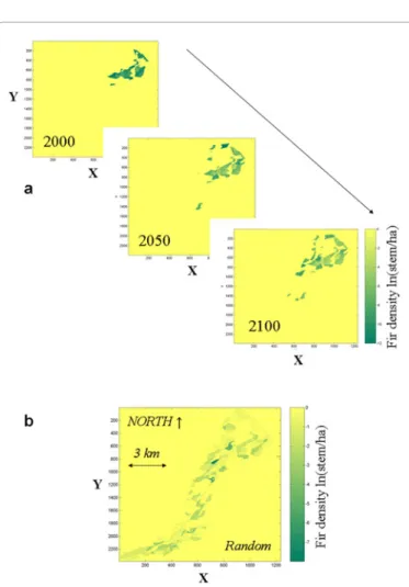
The studied site is located in the southeast of France, on the western slope of the Mont Ventou and the elevation is between ~900 and 1600 m. It consists in a forest sector managed by the French national forest service (ONF), with a mixture of species (Abies alba, P. nigra nigricans, Pinus sylvestris, P. uncinata and Fagus silvatica). Most of the real site is subject to active forestry management through thinning and natural or artificial regeneration, but further data are reduced only to natural evolutions. With a total surface area equal to 11.4 km², the site is made of 220 patches. The boundary coordinates of each patch i designed for the management purposes are delimited areas of roughly uniform stand densities d_i. The density is defined as the number of stems per hectare. As exhaustive data were not available over such a wide area and over such a long time period, I used the forest dynamics model CAPSIS [27] to simulate Fir trees and the four other species undergoing natural dynamics in a spatially explicit scheme. About 30 growth and yield models [28,29], mainly including stand-level models, diameter-class models and individual-based models have been integrated into the CAPSIS platform since 1999. The “VentouG” model, developed into the CAPSIS platform, performed a typical simulation hereafter called the reference (Figure 1a). VentouG is a semi-spatialized model (close to “gap-models”) that mixes diameter class growth models in a spatialized plot to study the natural evolution of heterogeneous forests evolving towards mixed stands [28,15].

VentouG simulations played the role of observations. This study analyzed the five species dynamics to illustrate how generic the approach is. In addition, I chose to focus on the Fir species (Abies alba) for a more detailed analysis. The dynamical distribution of Fir area is interesting: it is subject to colonization by seeds that come from important residual stands and is sensitive to elevation. We simulated here the evolving tree-densities of every patch according to processes of: i) colonization (exponential kernel dispersion, without external sources to the landscape); ii) regeneration (successive stage growth,

with regeneration heights comprised between 0.3 and 1.3 m); and iii) competition (mortality induced by local surroundings) between the stems of the five species [13,15]. All species mentioned above are simulated with the same processes, but with species-dependent calibration: they disperse (at a maximum distance between 1 to 2 km [30]), they have different fructification power and they compete with intra- as well as interspecies interactions. These ecological processes were explicitly applied on every stem, but no additional organizing processes such as large scale optimization were simulated. In general, simulations have shown a high sensitivity to dispersal, fructification and survival, especially at the seedling stage [28,29]. The run covered a period of 100 years with a time-step of 5 years and started with the real composition observed in year 2000. A fully random patchy landscape at the same site is shown for comparison (Figure 1b).

The landscape hamiltonian

I intended to characterize the landscape observations in terms of Hamiltonian functions. In order to detect a self-similar property of the reference landscape s, I first defined the Hamiltonian H function best characterizing the studied landscape [6]. H is defined using the exceedence probability P_E of tree-density differences ∆d between pairs

Figure 1: (a) Evolution of spatial distributions of Fir tree densities (stems/ha) in

the Mont Ventoux landscape. This multispecies site of about 1100 ha is called the reference landscape (only the Fir specie is displayed). Only year 2000 (observed), years 2050 and 2100 (simulated with the CAPSIS based process model) are shown, with the same coordinates and the same logarithmic colour scale. (b) The same landscape with hypothetical random tree densities is plotted for comparison and for visualizing patch boundaries.

(6)

Page 4 of 8 of patches for the whole landscape. In case of self-similar landscape,

this probability sets:

(

)

( )

1

E

P ∆ ≥d d ∝d− −τ (5) where τ-1 is the fractal dimension (the slope in loglog plot) of the P_E probability curve. Working here with exceedence probability allowed to characterize possible scaling behaviors as other cumulative functions would. The tree-density difference intended to capture ecological patch interactions.

In the empirical studies on river networks, minimization of an Hamiltonian given by equation (4), with γ = 0.5, showed that the exceedence probability distribution for areas obeyed a power law:

(

)

( )

1

E

P A a≥ ∝a− −τ , with τ-1 approximately equal to γ. By analogy with these works, we propose to define our landscape Hamiltonian as:

1

E

H P

∝ , with H_ij∝ ∆d_ijγ (6) where H_ij is the interaction strength (by analogy with physics, the potential or local force) associated to the tree-density difference ∆d_ij between patches i and j. For simplicity, this study supposed a direct proportionality (equality) between the left and the right part of both equations.

Finally, the total Hamiltonian value summarizing the whole landscape s leads to:

( )

T ij

i j

H s =

∑∑

H (7) Here again, the H_T value is by analogy with physics, the energy or the total “cost” of the landscape. Landscape energy has no clear meaning, but such function is a useful way to synthesize (to gather) all processes occurring in a landscape and leading to the tree-density pattern.

Practically, the H function used here is built from the fit made over fifty percentiles of the exceedence probability of observed tree-density differences. All tree-density differences between pairs of patches at every time step (2000 to 2100 with five a year step) for the reference landscape were computed separately. When computed separately at each time step, the H function shape remained relatively stable along time, but the information was too sparse in this case to cover many magnitude orders. Tree-density differences were then merged in order to extract an averaged H function that expressed the statistical behavior of the dynamic landscape. When H exhibits a self-similar shape, its associated γ exponent given by equation 1 and 2 was computed by fitting the histogram made of the 510510 observed density differences. The fit was obtained by a mean-squares procedure over the 20 to 200 main bins of the histogram. The final fit given by fifty bins was conserved, the others helping to compute the slope’s uncertainty. There were too ways for using the computed averaged H function: i) it was possible to compute the H_T value at every time step of the reference simulation and to characterize its regimes in time. For this purpose, I normalized all H_T values by the biggest value found in the species data; ii) it is possible to use this Hamiltonian to model a new landscape with similar statistical properties.

Modeling principle

Starting from the landscape Hamiltonian, it is possible to analyze the observed landscape or to simulate new (optimized) landscapes.

It has been demonstrated that it is easy to simulate landscapes using the Hamiltonian function by minimizing its total sum [6]. The minimization stage could be done with the T=0 Gibbs algorithm (i.e. Gibbs process by means of the Metropolis-Hastings algorithm) developed for physical systems studies [20,21,31] and recently applied in ecology too [13,32]. In an adaptation to patchy landscape interactions, it is expressed as follows: a) compute the total landscape valueH s_{T t}

( )

at step t using equation (7); b) randomly choose a patch within the landscape and randomly change its tree-density d_i (bounded

or not). Which consequently modifies all the tree-density differences

∆d_ij of pair-patches ij in which this selected patch i is involved; c) compute the new landscape valueH s_{T t}

( )

+₁ ; d) and finally compare

the latter to the previous H_T value. IfH s_{T t}

( )

+₁ ≤H s_{T t}

( )

, then keep this new configuration, otherwise keep the previous configuration, and reiterate at stage b); e) accept the convergence after n successless iterations (i.e. without any H_T decrease).

( )

, min T ij i j H s =

∑

∆dγ = (8) It has been demonstrated that this algorithm, also used in Bayesian framework, rapidly converges. No simulated-annealing has been performed in this preliminary study although it is possible and sometimes recommended.

This kind of optimization is a neutral model (NLM) in the sense that is requires very little information, namely the H function and the initial conditions (giving an averaged parameter value), and no ecological processes. In case of a self-similar landscape H possesses only one parameter: the γ exponent. Following hydrographical studies, this exponent connects local processes with an overall topological structure of the landscape (i.e. patch neighborhoods) such that: if 0 < γ << 1, we get a structured aggregation for which fine scales are dominant; if γ >> 1, the mosaic shows patch densities for which broad scale arrangements (ecological links) become dominant.

Starting from the observations (in fact, the CAPSIS mechanistic simulations), it is possible to compute the exceedence probability distribution, then helping to define the landscape Hamiltonian, finally allowing to analyze in turn the original observed landscape (arrow A) or to compute new optimized simulations (arrow B). The flow chart describes the successive stages of the calculation (Figure 2). A landscape analysis (A) consists in computing the evolution of the total H_T value of the observed landscape along to its dynamics (here over one century). Simulation study (B) was illustrated here by starting with the observed landscape of Mont Ventoux at year 2000, leading to a fully self-organized landscape at a posterior date. Simulation was made for the five species simultaneously and fir dynamics is analyzed in more detail. The dominant self-similar property was achieved after minimizing the H_T value of the evolving landscape. Iterations of the simulation were not supposed to correspond to any real time step. This NLM did not take into account patch elevations.

Results

Landscape hamiltonian

The exceedence probability of tree-density differences between pairs of patches of the Ventoux landscape as a function of tree-density differences exhibited a strong self-similarity (Figure 3). This directly comes from the ecological processes that we modeled (there is no minimization of H at this stage). Furthermore, the self-similarity

(7)

Page 5 of 8

Figure 2: Flow chart describing the successive stages of the calculation:

observations help to define the landscape Hamiltonian allowing to compute new simulations (arrow A) or to analyze the observed landscape (arrow B).

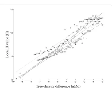
Figure 3: (a) Exceedence probability (noted PE) of the tree-density differences

against tree-density differences (Δd) presented in a loglog plot. 5000 dots were used in the original plot, while circles correspond to the fit with 50 regular bins. The same plot for the random landscape of figure 1b is shown for comparison, while its shape is highlighted with a linear fit (line, inset). (b) Hamiltonian function (noted H) extracted from the exceedence probability of the reference landscape. Here, dots correspond to open circles in figure 2. The slope γ of this loglog plot is highlighted with a mean-square linear fit.

Figure 4: Hamiltonian function computed from the exceedence probability

of the four other tree species involved into the reference landscape: P. nigra

nigricans (squares, dashed line); Pinus sylvestris (dots, doted-dashed line); P. uncinata (stars, doted line); Fagus silvatica (circles, plain line). Their respective

slopes of this loglog curve are highlighted with a mean-square linear fit.

covered up to nine (five in log₁₀) magnitude orders for all of the studied species (not shown). This extended scale range was accessible as a large landscape (220 patches, up to 12 km) and all time steps were merged for the analysis. It leaded to slopes equal to – γ = – 0.66; – 0.80; – 0.73; – 0.77; – 0.66 ± 0.02 for Abies alba, P. nigra nigricans, Pinus sylvestris, P. uncinata and Fagus silvatica respectively. Determination coefficients of these fits are roughly equal to r² = 0.97 ± 0.013, all significant (p <

10-5_{). Each uncertainty associated to the slope was the standard error}

computed on ten other fits with various numbers of histogram bins for each species. Figure 2a showed the result of this fit for the fifty bin case (Figure 3a circles) on an original diagram gathering 5000 bins (dots). As a reference, the same calculation was performed on the fully random mosaic: it did not show any self-similar behavior (Figure 3 inset).

Simply inverting this exceedence probability defined the Hamiltonian H function, in order to favor frequent tree-density differences (Figure 3b). The self-similar behavior detected here indeed indicated that low Fir density differences were more frequent in this landscape. H conserved the exceedence probability slope γ, while local

H values (i.e. associated to each pair-patch) are dimensionless. Taking

into account very high tree-density differences (extreme points at left in Figure 3a) or not did not change the fit. The four other species also exhibited strong self-similar behavior, with Hamiltonian slopes mentioned above and slightly higher than the one of fir species (Figure 4a).

Landscape analysis and simulation

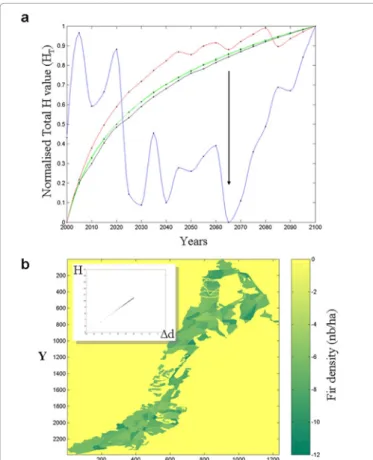
The evolution of the total H_T value of Fir landscape was quite variable over one century (Figure 5A). Higher H_T values corresponded to lower tree-density differences and thus to a more homogeneous landscape. There was a clear regime shift at year 2065, after which the fir Ventoux landscape tended to monotonously behave towards a more and more homogeneous landscape. Other species show more monotonous regimes, except maybe for Fagus silvatica starting to be limited by available elevations and competing species at the end of the simulation (Figure 5A). Such dynamics are also sensitive to past history that can vary from one species to another.

It was possible to model a landscape self-organization by using the previous H function deduced from the observed fir Ventoux landscape. The total H_T minimization procedure led to a new patchy landscape (Figure 5B). The final landscape was perfectly self-organized after only 300 iterations (calculations took a few seconds on a standard PC). The new Hamiltonian function extracted from the fir tree-density difference

(8)

Page 6 of 8 probabilities (equation (2)) was rigorously self-similar (Figure 5B inset)

and exhibited the same exponent as the one used in the Hamiltonian. Fir species filled almost all landscape patches as the NLM did not apply any elevation constraint, contrarily to the reference simulation.

Discussion

Optimized patchy landscapes

The five landscapes studied here appeared to be self-similar over more than nine (five in log₁₀) magnitude orders (Figure 4a). Data came from a spatially explicit process-based simulation of the Mount Ventoux site over a hundred years [27], thus extending data and allowing a complete control on the landscape generation mechanisms. The landscape evolution studied combined local processes such as colonization, competition and regeneration [15,30], without any additional organizing process. The landscape dynamic was characterised with the tree-densities of the 220 patches, and then the tree-density differences between all of the pair-patches to capture spatial interactions. The five mono-species landscapes exhibited self-similar behaviours, thus illustrating how generic the analysis might be. Their self-similar coefficients ranged from γ = 0.66 to 0.8, mainly due to dispersal and seedling stage survival differences between species. The (simple) way we used to estimate these coefficient values is not

important, as we did not try to infer processes underlying observed patterns. This main result strongly suggested that the combination of ecological processes behaves as a self organized landscape.

This observation fitted some others made in previous works [5,12]. For example, rural landscapes often hide a organization such as self-similar heterogeneity observed over temperate and tropical landscapes [10]. Furthermore, self-organization was interpreted in the present work as global optimization, as we minimized the landscape’s Hamiltonian. Indeed, starting from the observed tree-density distribution in space, it was possible to reconstruct a self-similar landscape using a potential force field summarising ecological interactions (Figure 5B). The landscape’s self-similar behaviour was the result of a global minimization of the sum of local landscape interactions, as was done in previous studies [25]. The self-similar behavior detected in the forested landscape was based on the observation that low tree density differences were more frequent, which fitted well with the concept of preferential attachment already mentioned to advocate optimizing patterns [8].

In addition to this interpretation of landscape generation, the optimization process opens a way to an original quantification of landscape features. This study showed how to characterize possible landscape regimes in time on the basis of the integrative Hamiltonian function (Figure 4a). The reference fir landscape studied here clearly showed a regime shift around year 2065 that was not explicitly modelled (Figure 5A). This shift could be the response of the colonization process to the spatial structure encountered in the landscape. The patch’s surroundings indeed favoured space exploration in a first stage, and tree-density smoothing (homogenization) in a second stage when the patches were already reached. The other species’ dynamics were rather different, more monotonous and smoother, due to different past histories and different calibrated processes (dispersion and mortality).

From a conceptual point of view, one needs to discuss the apparently remarkable fact that optimizing landscapes with respect to an Hamiltonian with parameter γ, always leads to a power-law for the excess probability distribution for density differences with parameter

γ

τ

−1

=

. The T=0 Metropolis algorithm we used drives the system into a local minimum of the Hamiltonian, so that there may not be a large departure from the initial condition (already showing an exceedence probability distribution with exponent γ). Yet, the global minimum of this Hamiltonian leads to the trivial and uniform distribution. Detailed studies of optimized river networks [33,34], analytically found the global minimum for the Hamiltonian given by equation (4): for all γ between 0 and 1, and different from 0 and 1, they found

τ-1 = 0.05.

This was confirmed by simulated annealing simulations, where the global minimum can effectively be found [26]. However, by using T=0 Metropolis algorithm with this Hamiltonian and γ =0.5, one visits the local minima with

τ-1 = 0.45

This value is in agreement with those measured in observed river networks. Such study and others led to the concept of “feasible optimality” according to which nature is “unable” to reach the true ground state (the global optimum) when complexity is involved. This could also be the case in patchy landscapes, given that one first checks how one can relate the Hamiltonian to ecological processes.

Some limits

The present NLM was in agreement with the parsimonious constraint of neutral models [13,14]. The strength of this parsimonious argument could also be a pitfall as the core of the method resides solely in the Hamiltonian H definition. If H is badly defined, the

Figure 5: Final computation steps described by the Fig. 2 flow chart. (A)

Normalized total HT values (i.e. the sum of Hamiltonian values over the whole

landscape) against the time steps (in years) of the reference landscape. There is a regime shift around year 2065. (B) Spatial distributions of Fir tree densities (stems/ha) of the Mont Ventoux landscape simulated by the Neutral Landscape Model on the basis of the Hamiltonian function of figure 3a. The inset (b) shows the resulting Hamiltonian function after simulation (similar to figure 2b) in loglog plot.

(9)

Page 7 of 8

NLM fails or even shows irrelevant landscape features. H is obviously highly dependent on the ecological parameter chosen to describe the landscape. In this forestry study, I focused on tree-density differences closely connected to ecological processes driving landscape dynamics. In other studies, cluster sizes of the vegetation cover were also used [9,11]. Agricultural landscapes for example are strongly dependent on the crop rotation system of farmers and would need other descriptive parameters. Finally, notice that NLM iterations were not directly linked to real time steps, even though this could be investigated if necessary [13]. Similarly, in a first stage here, I supposed a stationary over time H function, associated to an optimisation procedure towards steady-state or equilibrium (Figure 5B). This approximation could (and probably should) obviously be modified in a second stage of the description work of this landscape. This may be done either by forcing (driving) such Hamiltonian-based model or by defining dynamical rules of a new type.

Present computations were also underlying spatial assumptions. First, this work considered in a conservative approach all the existing pair-patches of the landscape (Figure 3), while different choices could be justified as well. For example, H could sum local interactions only coming from neighboring patches, with various (Delaunay or distance based) neighborhoods, as seen in other works [9,25]. Such choice depends on ecological processes advocated for landscape generation. Indeed I argue that the forest’s pattern under study involves different processes that could have long distance actions due to seed and pollen dispersion processes. Secondly, the patch’s definition may have played a role in such a landscape analysis. This weakness is common to every study in this field: studies focusing on vegetation cluster sizes also have to identify thresholds in order to define vegetation patches [9,12]. Patches were here defined by the sylvicultural management of Mont Ventoux landscape. I checked that slightly modified patch geometry (shapes and inter-distances) as well as topology (neighborhoods) did not change the present results. This is due to the fact that all pair-patches were taken into account for computations. Hence, the present method dedicated to Optimal Patchy Landscapes (OPL) seemed very robust in this sense. Thirdly, it is possible, and even probable, that additional processes influence the ecological pattern described here. We may modify or weight the Hamiltonian definition in order to take into account for the landscape topography, the soils, etc.

A dynamic landscape theory

There is presently little theory interpreting (not necessarily forested) landscape patterns and dynamics. Landscape ecology has been working on that point for a long time and is the origin of many powerful concepts such as heterogeneity [1]. Yet, there is still a lack of theoretical framework aiming at mechanistically interpreting landscape generating processes. No patchy landscape, the most common structure in rural areas, has been to my knowledge described with mathematical equations yet. In raster mode some composition analyses (i.e. averaged land cover percentages) were explored, while most of the landscape’s complexity resides in its configuration (its patch arrangements) and its dynamics [10]. Note that composition and configuration properties are highly dependent.

Recent works intended to explore landscape properties, but they often focused on “continuous” (raster) landscapes and did not succeed in giving clear explanations of observed scaling behaviour [9,12].

In this study, I investigated the same question with an ecologically based Hamiltonian function and its optimisation, thus following some pioneer works done on similar soap foams and tissue cells [21,23]. These authors exported a powerful model comprising almost all cells/units interactions into a Hamiltonian function and optional constraints to describe the evolution of the system. The Hamiltonian function is a way to summarise landscape properties within a simple equation (equation 2). By construction, the H function is intimately linked to various ecological processes such as colonization and competition involved in landscape generation. In this study, a higher H_T value corresponded to lower tree-density differences and to more homogeneous landscapes. Such homogenization could happen with “older” landscapes, stabilizing through a dominant colonisation process: colonizing species progressively fill the space and saturate it.

To put in a nutshell, this Hamiltonian function appears to be a fruitful theoretical framework to describe various landscapes. However it is still phenomenological (constructed by analogy with other problems) and its derivation from ecological processes is not known. In physical systems, this exponent connects local processes with the overall topological structure of the landscape (i.e. close and far away neighborhoods). Moreover, it is probable that the minimization procedure using a T=0 Metropolis algorithm only makes the landscape relaxed into a local or “metastable” state with respect to the Hamiltonian. It would be interesting to apply the present approach to observed landscapes: we could see how often they are self-organized in terms of various ecological parameters and what the observed γ exponent values are. Yet, it will certainly be difficult to gather the large amount of spatial and temporal data needed for this purpose. Such an analytical tool also gave the opportunity to compare landscapes (with a similar H function) or to study in depth complex landscape dynamics [3,35]. Following works on hydrographical systems [6], this theoretical framework potentially opens the way to a more complete dynamic landscape theory.

Acknowledgments

I warmly thank Fabien Campillo and Estelle Pitard for their comments on earlier drafts of this paper.

References

1. Forman RTT, Godron M (1986) Landscape ecology. John Wiley and sons (Eds), New York.

2. Turner MG, Gardner RH (1991) Quantitative methods in landscape ecology. Springer Verlag, New York.

3. Barbier N, Couteron P, Lejoly J, Deblauwe V, Lejeune O (2006) Self-organized vegetation patterning as a fingerprint of climate and human impact on semi-arid ecosystems. Journal of Ecology 94: 537-547.

4. Halley JM, Hartley S, Kallimanis AS, Kunin WE, Lennon JJ, et al. (2004) Uses and abuses of fractal methodology in ecology. Ecology Letters 7: 254-271. 5. Milne BT (1998) Motivation and benefits of complex systems approaches in

ecology. Ecosystems 1: 449-456.

6. Rodriguez-Iturbe I, Rinaldo A (1997) Fractal River Basins: Chance and Self-Organization. Cambridge University Press, New York, USA.

7. Stevens PS (1974) Patterns in nature. Little Brown & Co, Boston, USA. 8. D’Souza RM, Borgs C, Chayes JT, Berger N, Kleinberg RD (2007) Emergence

of tempered preferential attachment from optimization. Proceedings of the National Academy of Sciences of the United States of America 104: 6112-6117.

9. Scanlon TM, Caylor KK, Levin SA, Rodriguez-Iturbe I (2007) Positive feedbacks promote power-law clustering of Kalahari vegetation. Nature 449: 209-213.

(10)

Page 8 of 8

10. Gaucherel C (2009) Self-organisation of land cover heterogeneity in temperate and tropical landscapes. Ecological Complexity 6: 346-352.

11. Pascual M, Guichard F (2005) Criticality and disturbance in spatial ecological systems. Trends in Ecology & Evolution 20: 88-95.

12. Solé RV, Bascompte J (2006) Self-Organization in Complex Ecosystems. Princeton University Press, Princeton, USA.

13. Gaucherel C, Fleury D, Auclair D, Dreyfus P (2006) Neutral models for patchy landscapes. Ecological Modelling 197: 159-170.

14. With KA and King AW (1997) The use and misuse of neutral landscape models in ecology. Oikos 79: 219-229.

15. Dreyfus P, Pichot C, de Coligny F, Gourlet-Fleury S, Cornu G, et al. (2005) Couplage de modèles de flux de gènes et de modèles de dynamique forestière.

In Actes du 5ème colloque national du BRG « Un dialogue pour la diversité

génétique », Bureau des Ressources Génétiques, Lyon (France), pp. 231-250. 16. Gardner RH, Milne BT, Turnei MG, O’Neill RV (1987) Neutral models for the

analysis of broad-scale pattern. Landscape Ecology 1: 19-28.

17. Ising E (1924) Beitrag zur Theorie des Ferromagnetismus. Zeitschrift für Physik A Hadrons and Nuclei 31: 253-258.

18. Potts RB (1952) Some generalized order-disorder transformations. Mathematical Proceedings of the Cambridge Philosophical Society 48: 106-109.

19. Ashkin J and Teller E (1943) Statistics of two-dimensional lattices with four components. Phys Rev 64: 178-184.

20. Metropolis N, Rosenbluth AW, Rosenbluth MN, Teller AH, Teller E (1953) Equation of state calculations by fast computing machines. Journal of Chemical Physics 21: 1087-1092.

21. Sahni PS, Grest GS, Anderson MP, Srolovitz DJ (1983) Kinetics of the Q-State Potts Model in Two Dimensions Phys Rev Lett 50: 263-266.

22. Graner F, Glazier JA (1992) Simulation of biological cell sorting using a two-dimensional extended Potts model. Phys Rev Lett 69: 2013-2016.

23. Glazier JA, Balter A, Poplawski NJ (2007) Magnetisation to morphogenesis: A brief history of the Glazier-Graner-Hogeweg Model. In Anderson ARA, Chaplain

MAJ, Rejniak KA (eds.), Single-cell based models in biology and medicine, Birkhäuser Verlag, Basel (Switzerland), pp. 79-106.

24. Weitzman ML (1976) Income, Wealth, and the Maximum Principle. Harvard University Press, USA.

25. Rodriguez-Iturbe I, Ijjasz-Vasquez EJ, Bras RL, Tarboton DG (1992) Power Law Distributions of Discharge Mass and Energy in River Basins. Water Resources Research 28: 1089-1093.

26. Maritan A, Colaiori F, Flammini A, Cieplak M, Banavar JR (1996) Universality classes of optimal channel networks. Science 272: 984-986.

27. De Coligny F (2006) Efficient Building of Forestry Modelling Software with the Capsis Methodology. In PMA06 - Plant Growth Modelling and Applications, IEEE Computer Society, Los Alamitos, California (USA), pp. 216 - 222. 28. Courbaud B, Goreaud F, Dreyfus Ph, Bonnet FR (2001) Evaluating thinning

strategies using a tree distance dependent growth model: some examples based on the CAPSIS software “uneven-aged spruce forests” module. Forest Ecology and Management 145: 15-28.

29. Goreaud F, Alvarez I, Courbaud B, de Coligny F (2006) Long-term influence of the spatial structure of an initial state on the dynamics of a forest growth model: A simulation study using the capsis platform. Society for Computer Simulation International 82: 475-495.

30. Sagnard F, Pichot C, Dreyfus P, Jordano P, Fady B (2007) Modelling seed dispersal to predict seedling recruitment: Recolonization dynamics in a plantation forest. Ecological Modelling 203: 464-474.

31. Maes C, Redig F, Moffaert AV (2000) On the definition of entropy production, via examples. Journal of Mathematical Physics 41: 1528-1554.

32. Stoyan D, Stoyan H (1998) Non-homogeneous Gibbs process models for forestry- a case study. Biometrical Journal 5: 521-531.

33. Colaiori F, Flammini A, Maritan A, Banavar JR (1997) Analytical and numerical study of optimal channel networks. Phys Rev E 55: 1298-1310.

34. Sinclair K, Ball RC (1996) Mechanism for global optimization of river networks from local erosion rules. Phys Rev Lett 76: 3360-3363.

35. Couwenberg J, Joosten H (2005) Self-organization in raised bog patterning: the origin of microtope zonation and mesotope diversity. Journal of Ecology 93: 1238-1248.

Submit your next manuscript and get advantages of OMICS Group submissions

Unique features: • User friendly/feasible website-translation of your paper to 50 world’s leading languages • Audio Version of published paper • Digital articles to share and explore Special features: • 200 Open Access Journals • 15,000 editorial team • 21 days rapid review process • Quality and quick editorial, review and publication processing • Indexing at PubMed (partial), Scopus, DOAJ, EBSCO, Index Copernicus and Google Scholar etc • Sharing Option: Social Networking Enabled • Authors, Reviewers and Editors rewarded with online Scientific Credits • Better discount for your subsequent articles Submit your manuscript at: http://www.omicsonline.org/submission