• Aucun résultat trouvé

A shallow water with variable pressure model for blood flow simulation

N/A
N/A
Protected

Academic year: 2021

Partager "A shallow water with variable pressure model for blood flow simulation"

Copied!
23
0
0

Texte intégral

(1)

HAL Id: hal-01194326

https://hal.archives-ouvertes.fr/hal-01194326v2

Submitted on 12 Sep 2015

HAL is a multi-disciplinary open access

archive for the deposit and dissemination of

sci-entific research documents, whether they are

pub-lished or not. The documents may come from

teaching and research institutions in France or

L’archive ouverte pluridisciplinaire HAL, est

destinée au dépôt et à la diffusion de documents

scientifiques de niveau recherche, publiés ou non,

émanant des établissements d’enseignement et de

recherche français ou étrangers, des laboratoires

A shallow water with variable pressure model for blood

flow simulation

Olivier Delestre, Arthur Ghigo, Jose-Maria Fullana, Pierre-Yves Lagrée

To cite this version:

Olivier Delestre, Arthur Ghigo, Jose-Maria Fullana, Pierre-Yves Lagrée. A shallow water with variable

pressure model for blood flow simulation. Networks and Heterogeneous Media, AIMS-American

In-stitute of Mathematical Sciences, 2016, 11 (1), pp.69-87. �10.3934/nhm.2016.11.69�. �hal-01194326v2�

(2)

A shallow water with variable pressure model for

blood flow simulation

O. Delestre

, A.R. Ghigo

, J.-M. Fullana

and P.-Y. Lagr´

ee

§

September 12, 2015

Abstract

We performed numerical simulations of blood flow in arteries with a variable stiffness and cross-section at rest using a finite volume method coupled with a hydrostatic reconstruction of the variables at the interface of each mesh cell. The method was then validated on examples taken from the literature. Asymptotic solutions were computed to highlight the effect of the viscous and viscoelastic source terms. Finally, the blood flow was computed in an artery where the cross-section at rest and the stiffness were varying. In each test case, the hydrostatic reconstruction showed good results where other simpler schemes did not, generating spurious oscillations and nonphysical velocities.

1

Introduction

In this work we are interested in modeling and simulating blood flow in arteries with varying stiffness and cross-section. The blood flow in the main arteries of the systemic network is governed by the 3D Navier-Stokes equations which can be complicated and time-consuming to solve numerically. Fortunately, using well-known hypothesis valid in the case of blood flow in arteries (long wave approximation D/λ << 1, axial symmetry ∂θ= 0), this system of equations can

be simplified and then integrated over the cross-section of the artery in order to obtain a 1D hyperbolic system of equations, similar to the Saint-Venant system for shallow water flows. Details on the derivation of the model are presented in section (2) and can also be found in [23, 38]. Finally, we are left with a set of mass and momentum conservation equations with non dimensionless variables and parameters:    ∂tA + ∂xQ = 0 ∂tQ + ∂x  Q2 A + k 3√πρA 3/2  = √A πρ  ∂xA0− 2 3 √ A∂xk  − Cf Q A , (1)

Lab. J.A. Dieudonn´e & EPU Nice Sophia, University of Nice, France, e-mail :

de-lestre@math.unice.fr

CNRS and UPMC Universit´e Paris 06, UMR 7190, Institut Jean Le Rond d’Alembert,

France, e-mail : arthur.ghigo@dalembert.upmc.fr

CNRS and UPMC Universit´e Paris 06, UMR 7190, Institut Jean Le Rond d’Alembert,

France, e-mail : fullana@lmm.jussieu.fr

§CNRS and UPMC Universit´e Paris 06, UMR 7190, Institut Jean Le Rond d’Alembert,

(3)

with A(x, t) = πR(x, t)2 the cross-section area (R is the radius of the artery),

Q(x, t) = A(x, t)u(x, t) the discharge, u(t, x) the mean flow velocity, ρ the blood density, Cf the friction coefficient and A0 = k

A0 with k(x) the stiffness of

the artery and A0(x) = πR0(x)2the cross-section at rest.

The vast majority of arteries in the systemic network are tapered, meaning that the cross-section at rest A0(x) varies throughout the length of the artery.

Similarly, in the presence of arterial pathologies such as aneurysm or stenoses, the stiffness k (x) of the arterial wall can vary locally. As for shallow water equations with topography, the presence of tapper or variable stiffness in an artery modifies the blood flow, and both behaviors are accounted for in (1) through the source term A ( ∂xA0− 2

A∂xk/3 ) /

πρ. To numerically solve (1), it is necessary, among other things, to discretize this source term. A naive treatment of the topography gradients will most likely generate numerical os-cillations, therefore the use of the so-called well-balanced schemes is required to properly balance the fluxes and the source terms. In the following, we will focus on a specific well-balance method, called the hydrostatic reconstruction.

We will first present the derivation of the model and its properties, then the numerical method and in particular the derivation of the well-balanced scheme applied to the case of blood flow in arteries. We will then validate our method on examples taken from the literature and verify asymptotic behaviors of the numerical solution. Finally, we will compute the blood flow in an artery with varying cross-section and stiffness.

2

Derivation of the 1D blood flow equations

The 1D model for blood flow equations is derived from the conservative form of the Navier-Stokes equations for an incompressible fluid with constant viscosity µ:

∂tρ + ∇ρu = 0 (2)

∂tρu + ∇ · (ρuu + pI + τ ) = 0, (3)

where u is the velocity vector, ρ the density, supposed constant, p the pressure and τ the stress tensor to be defined. Using the control volume of the Figure

1, we integrate the Navier-Stokes equations over a volume V of cross-section A surrounded by a surface S (V = S ∪ A) and of length dz. We define then the average velocity U and pressure P as

{U, P } = 1 A

Z

∂A

{u, p}dA. From the mass conservation equation (2) we have:

Z ∂V (∇ρu)dV = Z ∂S ρu · ndS + Z ∂A ρu · ndA.

We then transform the volume integral using the Green (Divergence) theorem and writing the surface integral as S ∪ A. The surface element is dS = Rdθdz and the two terms are written as

Z ∂S ρu · ndS = 2π Z ur|RRdx = 2πρ Z ∂R ∂tRdx = ρ Z ∂A ∂tdx

(4)

x S dx V A2 A1

Figure 1: Control volume for integration (see text).

and Z

∂A

ρu · ndA = (ρAU )1− (ρAU )2=

Z d(ρAU ) = Z ∂x ∂ρAU ∂x , We retrieve therefore the first equation of our system

∂tA + ∂x(AU ) = 0.

For the conservation of momentum equation (3), the temporal term ∂tρu

be-comes Z ∂V ∂t(ρu)dV = ρ Z ∂V ∂tudAdx = ρ Z ∂x ∂t(U A)dx

and the divergence term R ∂V ∇ · (ρuu + pI + τ ) = Z ∂S (ρuu + pI + τ ) · ndS + Z ∂A (ρuu + pI + τ ) · ndA.

In the last two integrals the integration over the surface S is Z ∂S (ρuu + pI + τ ) · ndS = Z ∂S (pnx+ τrx)dS,

where the term uudS tends to zero. Finally, the integration over the area A gives

R

∂A(ρuu + pI + τ ) · ndA = [A(ρU

2+ P + τ xx)]21 = ρ Z ∂x ∂A(U2+ P/ρ) ∂x dx.

In terms of the cross-section A and the flow rate Q, we obtained the following system of equations: ∂tA + ∂xQ = 0 ∂tQ + ∂xQ 2 A = − A ρ∂xP − fv. (4)

(5)

The viscous effects are contained in fv which is computed by the integration

of the shear stress at the wall τrx over the internal surface dS. Therefore, it

depends on the exact flow condition. To close the mathematical problem we need a relation between the pressure P and the cross-section A, P = P (A), called the wall or state law. For fv = CfQ/A and the state law P = P0+

k (x) /√π(pA (x, t) − pA0(x)), which corresponds to the elastic response of

the artery, we obtain the proposed system of equations. (1).

3

Conservative hyperbolic system and steady states

Considering an artery with a constant stiffness k and a variable cross-section at rest A0(x), (1) reduces to the following system, similar to the shallow water

equations with topography:    ∂tA + ∂xQ = 0 ∂tQ + ∂x  Q2 A + k 3ρ√πA 3/2  = A ρ√π∂xA0− Cf Q A. (5)

As a reminder, the shallow water system is:    ∂th + ∂xq = 0 ∂tq + ∂x  q2 h + g 2h 2  = gh (S0− Sf) , (6)

with h(x, t) the water height, q(x, t) = h(x, t)u(x, t) the unit discharge, u(x, t) the mean flow velocity, g the constant of gravity, S0 = −∂xz the opposite of

the slope, z the topography and Sf the friction term (which takes the form of

Manning’s, Stickler’s, Ch´ezy’s, ... empirical friction law).

3.1

Hyperbolic system

The system (5) can be written using the following vectorial form:

∂tU + ∂xF (U ) = S(U ), (7)

where U is the vector of the conservative variables, F (U ) is the flux:

U =  A Q  , F (U ) =   Q Q2 A + k 3ρ√πA3/2   , (8)

and S(U ) is the source term, taking into account the shape of the vessel at rest A0(x) and the friction term

S(U ) =   0 A ρ√π∂xA0− Cf Q A   . (9)

The analogous term for the shallow water equations is the topography source term. The gradient of the flux (8) can be written as the product of the Jacobian

(6)

matrix J (U ) with the partial derivative of the vector of conservative variables U : ∂xF (U ) =   0 1 k√A 2ρ√π− Q2 A2 2Q A  .∂x  A Q  = J (U ).∂xU. (10)

When the cross-section A > 0, the Jacobian matrix admits two different real eigenvalues, λ1 and λ2: λ1= Q A− s k√A 2ρ√π = u − c and λ2= Q A + s k√A 2ρ√π = u + c, (11) with c the Moens-Korteweg wave propagation velocity (for the shallow water equations (6), c =√gh). In this case, the system is said to be strictly hyperbolic, which is a generalization of the advection phenomenon [18, 45, 30]: a part of the information concerning the flow propagates at the velocity λ1and the other

part at the velocity λ2. For blood flow under physiological conditions, we have

λ1> 0 and λ2< 0, hence the flow is subcritical.

3.2

Steady states

Since the works of [3,2] on the shallow water equations, it is well known that if a numerical scheme does not preserve steady states at the discrete level, spurious oscillations and artificial non zero velocities will be generated. The steady states for the system (5) are obtained when considering a stationary flow (i.e. there is no evolution in time) and are governed by the following equations:

   ∂xQ = 0 ∂x  Q2 2A2 + b √ A − bpA0(x)  = −Cf Q A2 , (12)

with b = k/(ρ√π) constant since we are considering an artery with a constant stiffness k. Neglecting the viscous friction effects (inviscid flow) by setting Cf =

0, we obtain the conservation of the discharge and Bernoulli’s law for blood flow:    Q = Q0 Q2 0 2A2 + b √ A − bpA0(x) = cst. . (13)

In the literature [8,37,44,6], we can find well-balanced numerical methods able to preserve the following steady state:

   q = q0 q2 0 2gh2+ h + z (x) = cst , (14)

which is the analogous of (13) in the case of the shallow water equations. How-ever, these methods are complicated to handle due to the occurrence of critical points when solving (13) or (14). Therefore we chose to focus on simpler steady states that we call the rest steady states or the ”man at eternal rest” equilib-rium [13] by analogy with the ”lake at rest” (introduced in [1]) or the hydrostatic equilibrium for the shallow water equations:


q = u = 0

∂x(h + z (x)) = ∂xη = 0 ,

(7)

where η is the water level. In this case we have a hydrostatic balance between the hydrostatic pressure and the gravitational acceleration. By analogy, we have the following equilibrium for the blood flow in arteries:

( Q = u = 0 ∂x  b√A − bpA0(x)  = 0 . (16)

Numerical methods able to preserve at least the steady states (16) are said to be ”well-balanced” since the work of [19]. A wide panel of well-balanced methods has been developed for shallow water equations. Among others we can mention [29,24,39,27,16,25,1,11,36,17,4,22,5,20]. In [13], we adapted the hydro-static reconstruction introduced in [1] to the system with constant stiffness (5). We will now present the hydrostatic reconstruction introduced in [1] adapted to the original system of equations (1) with varying stiffness k(x) and cross-section at rest A0(x). By a combination of the mass and momentum equations

in (1), under some regularity assumptions, we have: ∂tu + ∂x  u2 2 + 1 √ πρk (x) √ A −√1 πρA0(x)  = −Cf Q A2, (17)

with A0(x) = k (x)pA0(x). Considering a stationary flow where the viscous

friction is neglected by setting Cf = 0, we recover Bernoulli’s law (13). The

notable difference is that k is now a function of x. In the case of the ”man at rest” equilibrium” (without artifacts such as [26,35]) we obtain:

( Q = u = 0 ∂x  k (x)√A − A0(x)  = 0 . (18)

The fact that now k is a function of x will influence the way the well-balanced scheme is obtained. In the following section, we will present a well-balanced scheme for system (1), based on the hydrostatic reconstruction for Saint-Venant/shallow water equations with variable pressure [5].

4

The numerical method

4.1

Numerical context

Several numerical methods have been used to solve the blood flow equations. In [43], they are solved thanks to the Methods of Characteristics (MOC). In [51,50], they use a conservative form of the model

   ∂tA + ∂x(Au) = 0 ∂tu + ∂x  u2 2 + P ρ  = −Cf Q A2 , (19)

with the non-conserved vector (A, u) and equations (19) are solved with a two-step Lax-Wendroff scheme. In [42], a quasi conservative form of the equations (with s(U ) a source term)

   ∂tA + ∂xQ = 0 ∂tQ + ∂x  Q2 A  +A ρ∂xp = s(U ) , (20)

(8)

is solved thanks to a first order explicit in time upwind finite difference scheme. In [38], they are the first to solve blood flow equations under a conservative form, thanks to a two-step Lax-Wendroff scheme. The solutions of the equations under the form (19) using an upwind Discontinuous Galerkin method (used by [49,48]) and a Taylor Galerkin finite element method (also used in [33,14,34]) have been compared in [41]. A MacCormack finite difference method has been applied in [15] followed by [40]. Finite volume methods seem to be first used to solve these equations in [9, 10]. In [13], a well-balanced finite volume method based on the hydrostatic reconstruction (introduced in [1]) is applied on system (5), and this method is compared with a Taylor Galerkin method in [46]. We will present in the following sections the extension of the well-balanced scheme (based on an extension of the hydrostatic reconstruction) we have used to solve the system (1), which can be written under the following vectorial form

∂tU + ∂xF (U, Z) = S1(U, Z) + S2(U ), (21) with U =  A Q  , Z =  A0 k  , F (U, k) =   Q Q2 A + 1 3√πρkA 3/2   , (22)

and the source terms

S1(U, Z) =   0 A √ πρ  ∂xA0− 2 3 √ A∂xk    and S2(U ) = 0 −Cf Q A ! . (23)

4.2

Convective step

For the homogeneous system

∂tU + ∂xF (U, Z) = 0 (24)

which is (21) without source term, an explicit first order in time conservative scheme can be written as:

Uin+1− Un i ∆t + Fn i+1/2− F n i−1/2 ∆x = 0, (25)

where i refers to the cell Ci= (xi−1/2, xi+1/2) = (xi−1/2, xi−1/2+ ∆x) and n to

time tn with tn+1− tn= ∆t. Uin is an approximation of U :

Uin' 1 ∆x Z xi+1/2 xi−1/2 U (x, tn)dx , and Fi+1

2 is an approximation of the flux function F (U, Z) at the cell interface

i + 1/2

Fi+1/2n = F(Uin, Ui+1n , Zi, Zi+1).

(9)

4.3

Source terms treatment

4.3.1 Topography source term S1(U, Z)

In the system (21), the term S1(U, Z) is involved in the steady state

preserva-tion, therefore requires a well-balanced treatment. Following a variant of the hydrostatic reconstruction [5, p.93-94], the variables are reconstructed locally from (18) on both sides of the interface i + 1/2 of the cell Ci:

       pAi+1/2L= max(ki √

Ai+ min(∆A0i+1/2, 0), 0)/ki+1/2∗

Ui+1/2L= (Ai+1/2L, Ai+1/2L.ui)t

pAi+1/2R= max(ki+1pAi+1− max(∆A0i+1/2, 0), 0)/k∗i+1/2

Ui+1/2R= (Ai+1/2R, Ai+1/2R.ui+1)t,

(26)

with ∆A0i+1/2= A0i+1−A0i= ki+1pA0i+1−ki

A0iand k∗i+1/2= max(ki, ki+1).

In order to help the understanding of the principle of the hydrostatic recon-struction (26), we present the hydrostatic reconstruction for the shallow water system of equations (6):       

hi+1/2L= max(hi+ zi− zi+1/2, 0)

Ui+1/2L= (hi+1/2L, hi+1/2L.ui)t

hi+1/2R = max(hi+1+ zi+1− zi+1/2, 0)

Ui+1/2R= (hi+1/2R, hi+1/2R.ui+1)t,

(27)

with zi+1/2 = max(zi, zi+1). The water height is reconstructed in a way that

allows to have locally the hydrostatic equilibrium h + z = cst on each side of the interface i + 1/2. As mentioned in [1], max(., 0) is there to ensure the positivity of the water height in case of drying and the upwind evaluation of zi+1/2ensures

that 0 ≤ hi+1/2L ≤ hi and 0 ≤ hi+1/2R ≤ hi+1, which has been proved in [1]

to ensures the positivity of the water height. For blood flow equations with a constant stiffness k, the corresponding equilibrium writes√A −√A0= cst, so

A (respectively −√A0) ”plays the role” of h (resp. z), thus in that case the

hydrostatic reconstruction writes:        pAi+1/2L= max( √ Ai− √ A0i+pA0i+1/2, 0)

Ui+1/2L= (Ai+1/2L, Ai+1/2L.ui)t

pAi+1/2R = max(pAi+1−pA0i+1+pA0i+1/2, 0)

Ui+1/2R = (Ai+1/2R, Ai+1/2R.ui+1)t.

(28)

As we have −√A0instead of z, we take pA0i+1/2= min(

√ A0i,pA0i+1), thus we have:        pAi+1/2L= max( √ Ai+ min(∆ √ A0i+1/2, 0), 0) Ui+1/2L= (Ai+1/2L, Ai+1/2L.ui)t

pAi+1/2R = max(pAi+1− max(∆

A0i+1/2, 0), 0) Ui+1/2R = (Ai+1/2R, Ai+1/2R.ui+1)t,

(29)

with ∆√A0i+1/2=pA0i+1−

A0i. We can notice that we recover reconstruc-tion (29) if the stiffness k is constant in reconstruction (26). For consistency, the scheme (25) is modified as follows:

Uin+1= Uin− ∆t ∆x  Fi+1/2Ln − Fn i−1/2R  , (30)

(10)

where Fn i+1/2L= F n i+1/2+ Si+1/2L, Fn i−1/2R= F n i−1/2+ Si−1/2R, with

Fi+1/2n = FUi+1/2L, Ui+1/2R, k∗i+1/2

 , Si+1/2L=  0 P(An i, ki) − P(Ani+1/2L, k ∗ i+1/2)  , Si−1/2R=  0 P(An i, ki) − P(Ani−1/2R, k ∗ i−1/2)  ,

and P(A, k) = k (x) A3/2/(3ρπ). Thus blood flow in a artery with varying

cross-section at rest and stiffness is treated in a well-balanced way.

4.3.2 Viscous source term S2(U )

In system (21), the friction term −CfQ/A in S2(U ) is treated semi-implicitly.

This treatment is classical in shallow water simulations [7, 31] and has proven efficient in blood flow simulation as well [13]. Furthermore, this treatment preserves the ”dead man” equilibrium (18). It consists in using first (30) as a prediction step without friction, i.e.:

Ui∗= Uin− ∆t ∆x  Fi+1/2Ln − Fn i−1/2R  ,

then applying a semi-implicit friction correction on the predicted values (Ui∗):

A∗i  u n+1 i − u ∗ i ∆t  = −Cfun+1i .

Thus we get the corrected velocity un+1i and we have An+1i = A∗i.

4.4

HLL numerical flux

As presented in [13], several numerical fluxes can be used (Rusanov, HLL, VFRoe-ncv and kinetic fluxes) for numerical simulations of blood flow in ar-teries. Details can be found in [5, 12, 13]. In this work we will use the HLL flux (Harten Lax and van Leer [21]) because it is the best compromise between accuracy and CPU time consumption (see [12, chapter 2]). It writes:

F(UL, UR, k∗) =        F (UL, k∗) if 0 ≤ c1 c2F (UL, k∗) − c1F (UR, k∗) c2− c1 + c1c2 c2− c1 (UR− UL) if c1< 0 < c2 F (UR, k∗) if c2≤ 0 , with c1= inf U =UL,UR ( inf j∈{1,2}λj(U, k ∗)) and c 2= sup U =UL,UR ( sup j∈{1,2} λj(U, k∗)),

where λ1(U, k∗) and λ2(U, k∗) are the eigenvalues of the system and k∗ =

(11)

To prevent a blow up of the numerical values, we impose the following CFL (Courant, Friedrichs, Lewy) condition:

∆t ≤ nCF L ∆x max i (|ui| + ci) , where ci= p ki √ Ai/(2ρ √ π) and nCF L= 1.

5

Validation of the method

To validate the well-balanced scheme presented in the previous sections for blood flow in arteries with varying stiffness k (x) and cross-section at rest A0(x), we

applied it to different test cases taken from [13], where arteries with a varying cross-section at rest A0(x) and a constant stiffness k were considered. For each

of these examples, the rest equilibrium state was: Q = 0 and √A −√A0 = 0

and non-reflecting boundary conditions were set at each end of the computa-tional domain in the form of homogeneous Neumann boundary conditions. The hydrostatic reconstruction scheme as well as a naive centered discretization of the source term were systematically tested to clearly evaluate the benefit of us-ing a well-balanced scheme. Accordus-ing to [13], several Riemann solvers can be used, but we only display results obtained using the HLL flux. In the following, we present the numerical parameters, the analytic solution if it exists and the numerical results. For further details we refer the reader to [13].

5.1

”The man at eternal rest”

We considered an artery at its equilibrium state, where there is no flow and the radius of the cross-section at rest R0(x) varies throughout the artery, as for

example in a dead man with an aneurysm. This equilibrium state is exactly the one well-balanced methods are designed to preserve. If the topography source term is not treated correctly, non-physical velocity may be generated.

We used the following numerical values: L = 0.14 m, J = 50 cells, Tend =

5 s, ρ = 1060 kg.m−3, Cf = 0 and k = 4.0 × 10⁸ P a.m−1. We used the

equilibrium state as an initial condition, setting Q(x, 0) = 0 and:

R (x, 0) = R0(x) =                        R0 if x ∈ [0, x1] R0+ ∆R 2  1 + sin  −π 2 + π  x − x1 x2− x1  if x ∈ ]x1, x2[ R0+ ∆R if x ∈ [x2, x3] R0+ ∆R 2  1 + cos  π x − x3 x4− x3  if x ∈ ]x3, x4[ R0 if x ∈ [x4, L] , with R0 = 4.0 × 10⁻³ m, ∆R = 1.0 × 10⁻³ m, x1 = 1.0 × 10⁻² m, x2 =

3.05 × 10⁻²m, x3= 4.95 × 10⁻²m and x4= 7.0 × 10⁻²m. The radius at rest

(12)

The results obtained are presented in Figure 2 right. As expected, a naive centered discretization of the topography source term results in nonphysical os-cillations of the velocity u (x, t), whereas the well-balanced solution preserves the equilibrium state.

0.0036 0.0038 0.004 0.0042 0.0044 0.0046 0.0048 0.005 0.0052 0.0054 0 0.02 0.04 0.06 0.08 0.1 0.12 0.14 R [m] x [m] R0 -1.5 -1 -0.5 0 0.5 1 1.5 0 0.02 0.04 0.06 0.08 0.1 0.12 0.14 u [m/s] x [m] Hydrostatic reconstruction Centered discretization

Figure 2: The ”dead man case”: (Left) The radius of the artery R0(x); (Right)

Comparison of the velocity at time t = 5 s between an explicit treatment of the source term (dashed line) and the hydrostatic reconstruction (full line).

5.2

The ideal ”Tourniquet”

This test case is the equivalent of the dam break problem for the Shallow Water equations (Stoker’s solution in [12]). We considered an artery with a constant radius at rest R0, a constant stiffness k and no viscous friction (Cf = 0),

there-fore the governing system of equations was (24). Initially, a tourniquet was applied and then immediately removed. We have a Riemann problem and the method of characteristics allowed us to compute an analytic solution that we compared to the numerical solutions. This Riemann problem has been first in-troduced in compressible gas dynamic with the Sod tube (for further details we refer the reader to [28,32]) and extended to blood flow in [13].

We considered an artery of length L = 8.0 × 10⁻²m with x ∈−L2,L2 and used the following numerical parameters: J = 100 cells, Tend = 5.0 × 10⁻³ s,

ρ = 1060 kg.m−3 and k = 1.0 × 10⁷ P a.m−1. We used a perturbation of the

equilibrium state as an initial condition, setting Q(x, 0) = 0 and:

A (x, 0) =        AL=π (R0+ ∆R) 2 if x ∈  −L 2, 0  AR=πR20 if x ∈  0,L 2  , with R0= 4.0 × 10⁻³m and ∆R = 1.0 × 10⁻³m.

(13)

The results obtained are presented in Figure 3. We can see that the nu-merical solution obtained with the well balanced scheme is in good agreement with the analytic solution presented in [13]. This is also true for the solution obtained using a centered discretization of the topography source term, which is superposed on the well-balanced solution, since in this case the source term is null. 0.004 0.0042 0.0044 0.0046 0.0048 0.005 -0.04 -0.03 -0.02 -0.01 0 0.01 0.02 0.03 0.04 R [m] x [m] Exact Hydrostatic reconstruction Centered discretization 0 2x10⁻⁵ 4x10⁻⁵ 6x10⁻⁵ 8x10⁻⁵ 0.0001 -0.04 -0.03 -0.02 -0.01 0 0.01 0.02 0.03 0.04 Q [m 3/s] x [m] Exact Hydrostatic reconstruction Centered discretization

Figure 3: The Tourniquet: (Left) Radius of the artery R (x) at t = 5 × 10⁻³ s; (Right) Flow rate of the artery Q(x) at t = 5 × 10⁻³s. Comparison between the exact analytic solution (full line) and the numerical solution obtained with an explicit treatment of the topography source term and the hydrostatic recon-struction (dashed lines). The numerical solutions are superposed.

5.3

Wave reflection-transmission of the pulse towards a

constriction

In this section we considered the propagation of a pulse towards constriction. This configuration is an idealized representation of a transition between a parent artery and a daughter artery of smaller cross-section. We tested here the ability of the numerical scheme to capture the propagation of a small perturbation of the equilibrium state at the beginning of an artery with a varying radius at rest R0(x). In order to accurately compute the numerical solution, the forward

and backward traveling waves need to be correctly captured as well as the re-flected and transmitted waves generated by the abrupt change in topography at the transition point. To test if these reflections were accurately described, we computed the analytic reflection and transmission coefficients at the transition point and compared them to the amplitude of the numerical reflected waves. For further details we refer the reader to [13].

We considered an artery of length L = 0.16 m and used the following numer-ical parameters: J = 1500 cells, Tend= 8.0 × 10⁻³s, ρ = 1060 kg.m−3, Cf= 0

and k = 1.0 × 10⁸P a.m−1. The constriction was defined by the following radius

(14)

R0(x) =          RR+ ∆R if x ∈ [0, x1] RR+ ∆R 2  1 + cos  πx − x1 x2− x1  if x ∈ ]x1, x2] RR if x ∈ ]x2, L] ,

with RR = 4.0 × 10⁻³m, ∆R = 1.0 × 10⁻³ m, x1= 1940L and x2= L2. We set

Q(x, 0) = 0 as an initial condition and we defined the initial perturbation as:

R (x, 0) =      R0(x)  1 +  sin 100 20Lπ (x − x3)  if x ∈ [x3, x4] R0(x) else ,

with x3 = 10015L < x1, x4 = 10035L < x2 and  = 5.0 × 10⁻³ a small parameter

ensuring that we stayed in the range of small perturbations of the equilibrium state.

The numerical results are plotted in Figure4. We can see that the propaga-tion of the pulse as well as the wave reflecpropaga-tions and transmissions are accurately described using the well balanced scheme (Figure4left) whereas spurious waves appear with the centered discretization of the source term (Figure4 right).

-5e-06 0 5e-06 1e-05 1.5e-05 2e-05 2.5e-05 0 0.02 0.04 0.06 0.08 0.1 0.12 0.14 0.16 R-R 0 [m] x [m] εR0/2 εR0Tr/2 εR0Re/2 t=0 t=T/4 t=3T/4 -1e-05 -5e-06 0 5e-06 1e-05 1.5e-05 2e-05 2.5e-05 0 0.02 0.04 0.06 0.08 0.1 0.12 0.14 0.16 R-R 0 [m] x [m] εR0/2 εR0Tr/2 εR0Re/2 t=0 t=T/4 t=3T/4

Figure 4: (Left) Hydrostatic reconstruction; (Right) Centered discretization of the topography source term. R(x) − R0(x) at 3 time steps: t = 0, t = Tend4 , t =

3Tend

4 . The straight dashed lines represent the level of the predicted reflection

(Re) and transmission (Tr) coefficients.

6

Asymptotic solutions for a uniform vessel

In this section we studied the propagation of a pulse wave in a uniform vessel (k = cst, A0 = cst) and derived asymptotic solutions of the system of equation

(1), following the work of Wang and al. [47]. Small perturbations ˜Q, A0+  ˜A

(15)

of the base state (Q = 0, A = A0) were considered, resulting in the following

linearized system of equations:      ∂tA + ∂˜ xQ = 0˜ ∂tQ + c˜ 20∂xA = −C˜ f ˜ Q A0 , (31)

where c0=pkR0/ (2ρ) is the Moens-Korteweg celerity.

In the following numerical examples, we only present results obtained for the hydrostatic reconstruction since we considered a uniform vessel. The nu-merical parameters were defined as follows: L = 3 m, R0 = 1.0 × 10⁻² m,

J = 1500 cells, Tend = 0.5 s, ρ = 1060 kg.m−3, µ = 3.5 × 10⁻³ P a.s and

k = 1.0 × 10⁷ P a.m−1. The parameters C

f and Cv, respectively the viscous

coefficient and the viscoelastic coefficient, were set according to the desired test case.

Initially, the system was at its equilibrium state Q = 0, A = A0= πR20 and

an inflow boundary condition was prescribed as Q (x = 0, t) = Qin(t) with:

Qin(t) = Qcsin( 2π Tc t) H  −t +Tc 2  , t > 0 ,

where H(t) is the Heaviside function, Tc the period of the sinusoidal wave and

Qcthe maximum amplitude of the inflow wave. We set Qc= 1.0 × 10⁻⁶m3.s−1

and Tc= 0.4 s to insure that only small perturbations from the equilibrium state

were considered. The cross-section at the inlet A(x = 0, t) was reconstructed by a matching of the outgoing characteristic, technique that takes advantage of the hyperbolic nature of the problem. A homogeneous Neumann boundary condi-tion was prescribed at the outlet to simplify the computacondi-tion of the asymptotic solutions and to avoid reflections.

6.1

The d’Alembert equation

Following ideas developed in [47], we set Cf = 0 in (31) and we obtained the

d’Alembert equation, which admits the following pure wave solution c0A˜0 =

˜

Q = Qin(x − c0t).

In Figure5, we can see the propagation of a pulse wave without dissipation or diffusion, as predicted by the analytic solution.

6.2

Dissipation due to the viscosity of the blood

We also investigated the effect of the blood viscosity on the propagation of the pulse wave and set Cf 6= 0. Starting from the linearized system of equations

(31), we considered the small parameter f = TcCAf

0 and performed the change

of variables ξ = x − c0t and τ = ft to place ourselves in the moving frame at

slow times to properly capture the effects of the viscous term. The first order solution obtained in [47] is:

(16)

0 0.001 0.002 0.003 0.004 0.005 0 0.5 1 1.5 2 2.5 3 u [m] x [m] t=0.1s t=0.2s t=0.3s t=0.4s t=0.5s

Figure 5: Pure wave solution: u (x) at time t = {0.1, 0.2, 0.3, 0.4, 0.5} for the well-balanced scheme. The straight black dotted line represents the maximum amplitude of the pure wave solution.

c0A˜0= ˜Q0= ˜Q0(x − c0t) exp  −f t 2Tc  , where exp−f2Ttc 

is the exponential envelop of the pure wave solution ˜Q0(x − c0t).

To obtain this asymptotic solution numerically, we set Cf = 40πν = 4.15 ×

10−4m2.s−1, therefore f = 0.53.

In Figure 6, we can see the propagation of the pulse with dissipation (or attenuation) of its amplitude due to the viscosity of the blood. The straight doted line represents the exponential envelop exp−f2Tx

cc0


computed previ-ously and is in good agreement with the decrease in amplitude of the pulse wave. One can note that as expected, there is no diffusion, since the wavelength of the pulse does not change while it propagates in the artery.

6.3

Diffusion due to the viscoelasticity of the arterial wall

In this section, we set the friction coefficient to zero (Cf = 0) and focused on an

other important characteristic of the blood flow in the arteries: the viscoelastic-ity of the arterial wall. We chose here to take into account this time-dependent behavior in our governing system of equations through a very simple lumped model, the Kelvin-Voigt model, resulting in an additional parabolic term in the governing system of equations:

   ∂tA + ∂xQ = 0 ∂tQ + ∂x  Q2 A + k 3√πρA 3/2  = −Cf Q A + Cv∂ 2 xQ , (32)

where the viscoelastic coefficient Cν is defined as Cν = 23 φh

ρR0 = 1.57 m

2.s−1

with φ = 5000 P a.s and h = 5.0 × 10⁻³ m. The parabolic term was treated by performing a temporal splitting of the problem. First the purely hyperbolic

(17)

0 0.001 0.002 0.003 0.004 0.005 0 0.5 1 1.5 2 2.5 3 u [m] x [m] t=0.1s t=0.2s t=0.3s t=0.4s t=0.5s

Figure 6: Viscous damping: u (x) at time t = {0.1, 0.2, 0.3, 0.4, 0.5} for the well-balanced scheme. The straight black dotted line represents the exponential envelop of the asymptotic solution.

problem with a non reflecting boundary condition at the outlet was solved, and its solution was then used as an initial condition of the parabolic problem. A Crank-Nicolson scheme coupled with homogeneous Neumann boundary condi-tions was than used to solve the parabolic problem.

To correctly capture the behavior of this new viscoelastic term, we defined a new small parameter ν = cC2v

0Tc = 8.3 × 10

−2 and applied the same technique

as in the previous section. From [47] we have the following first order diffusive analytic solution, which is a solution of the heat equation:

       ˜ Q0(τ, ξ) = Z ∞ −∞ ˜ Q0(0, η) G (τ, ξ − η) dη G(τ, ξ) = 1 p2πτ c2 0Tc e−ξ2/(2τ c20Tc) .

The numerical results for several times and the analytic solution at t = 0.4 s are presented in Figure 7. We can see that the viscoelastic term induces a diffusion of the pulse wave, changing its wavelength, and that the numerical solution at t = 0.4 s perfectly matches with the asymptotic solution at t = 0.4 s.

7

Real artery simulation

In this section, we focused on simulating the propagation of a pulse wave in a tapered artery of length L = 3 m, where the the radius of the cross section at rest R0(x) was linearly decreasing from the proximal to the distal end of the

artery: R0(x) =      RL if x ∈ [0, x1[ RL− (x − x1)∆R if x ∈ [x1, x2[ RL− (x2− x1)∆R if x ∈ [x2, L[ ,

(18)

0 0.001 0.002 0.003 0.004 0.005 0 0.5 1 1.5 2 2.5 3 u [m] x [m] t=0.1s t=0.2s t=0.3s t=0.4s t=0.5s analytic t=0.4s

Figure 7: Viscoelastic diffusion: u (x) at time t = {0.1, 0.2, 0.3, 0.4, 0.5} for the well-balanced scheme (dashed lines). The black dotted line represents the asymptotic solution at t = 0.4 s.

with RL= 4.0 × 10⁻³m, ∆R = 1.0 × 10⁻³m, x1=204L and x2=1620L.

Follow-ing [47], the stiffness of the arterial wall was defined as k(x) = 43REh2 0(x)

with E the Young’s modulus and h the width of the arterial wall. Therefore we were in a configuration where R0and k were varying throughout the length of the artery

and if the well-balanced scheme was not used, spurious waves might have arisen. We used the following numerical parameters to mimic the geometrical and mechanical properties of a real artery: J = 1500 cells, Tend = 0.5 s, ρ =

1060 kg.m−3, µ = 3.5 × 10⁻³ P a.s, E = 4.0 × 10⁵ P a, h = 5.0 × 10⁻⁴ m,

Cf = 8πν, φ = 5000 P a.s and Cv = 23ρRφh0. We used the same initial inflow

condition as for the asymptotic solutions.

-0.01 0 0.01 0.02 0.03 0.04 0.05 0 0.5 1 1.5 2 2.5 3 u [m] x [m] t=0.1s t=0.2s t=0.3s t=0.4s t=0.5s -0.01 0 0.01 0.02 0.03 0.04 0.05 0 0.5 1 1.5 2 2.5 3 u [m] x [m] t=0.1s t=0.2s t=0.3s t=0.4s t=0.5s

Figure 8: Tapered artery - Pure wave solution: u (x) at time t = {0.1, 0.2, 0.3, 0.4, 0.5} for Cf = 0 and Cν = 0: (Left) Centered discretization

(19)

-0.01 0 0.01 0.02 0.03 0.04 0.05 0 0.5 1 1.5 2 2.5 3 u [m] x [m] t=0.1s t=0.2s t=0.3s t=0.4s t=0.5s

Figure 9: Tapered artery: viscous and viscoelastic effects: u (x) at time t = {0.1, 0.2, 0.3, 0.4, 0.5} for the well-balanced scheme.

The results are presented in figures8and9. We can see that in the absence of friction and viscoelastic effects (figure8), if the well-balanced scheme is not used (figure 8 left) nonphysical reflections appear. On the contrary, the well-balanced scheme provides a satisfactory numerical solution, where a continuous reflection phenomena takes place due to the tapering, resulting in a decrease of the amplitude of the backward traveling wave and an increase of the amplitude of the forward traveling wave. Indeed, in the case of a tapered artery, the transmission coefficient Tr > 1 and the reflection coefficient Re < 1. When

viscous and viscoelastic effects are taken into account (figure9), all phenomena add up and we recognize the effects of the continuous reflection, the viscous dissipation and the viscoelastic diffusion.

Conclusion and perspectives

In this work we have presented a numerical method based on a well-balanced finite volume scheme for the blood flow equations with variable wall elasticity. This scheme based on an extension of the hydrostatic reconstruction gave very good results on several tests, for which classical methods failed. In further work, we will try to improve the accuracy of the numerical method by raising the order of the numerical method and to apply this method to real network modeling.

Acknowledgments

The first author would like to thanks the organizers of the international confer-ence CoToCoLA to offer the opportunity to communicate in the framework of this conference which took place in Besan¸con city from the 9th to the 12th of February 2015.

(20)

References

[1] E. Audusse, F. Bouchut, M.-O. Bristeau, R. Klein, and B. Perthame, A fast and stable well-balanced scheme with hydrostatic reconstruction for shallow water flows, SIAM J. Sci. Comput., 25(6), (2004), 2050–2065. [2] A. Berm´udez, A. Dervieux, J.-A. Desideri, and M. E. V´azquez, Upwind

schemes for the two-dimensional shallow water equations with variable depth using unstructured meshes, Computer Methods in Applied Mechanics and Engineering, 155(1-2), (1998), 49–72.

[3] A. Berm´udez and M. E. V´azquez, Upwind methods for hyperbolic con-servation laws with source terms, Computers & Fluids, 23(8), (1994), 1049–1071.

[4] C. Berthon and F. Foucher, Efficient well-balanced hydrostatic upwind schemes for shallow-water equations, Journal of Computational Physics, 231, (2012), 4993–5015.

[5] F. Bouchut, Nonlinear stability of finite volume methods for hyperbolic conservation laws, and well-balanced schemes for sources, volume 2/2004, Birkh¨auser Basel, 2004.

[6] F. Bouchut and T. Morales De Luna, A subsonic-well-balanced reconstruc-tion scheme for shallow water flows, SIAM J. Numer. Anal., 48(5), (2010), 1733–1758.

[7] M.-O. Bristeau and B. Coussin, Boundary conditions for the shallow water equations solved by kinetic schemes, Technical Report 4282, INRIA, 2001. [8] M. J. Castro, A. Pardo, and C. Par`es, Well-balanced numerical schemes based on a generalized hydrostatic reconstruction technique, Mathematical Models and Methods in Applied Sciences, 17(12), (2007), 2065–2113. [9] N. Cavallini, V. Caleffi, and V. Coscia, Finite volume and WENO scheme

in one-dimensional vascular system modeling, Computers and Mathematics with Applications, 56, (2008), 2382–2397.

[10] N. Cavallini and V. Coscia, One-dimensional modeling of venous patholo-gies: Finite volume and WENO schemes, in Advances in Mathematical Fluid Mechanics (eds, R. Rannacher and A. Sequeira), Springer Berlin Heidelberg, (2010), 147–170.

[11] T. Chac´on Rebollo, A. Dom´ınguez Delgado, and E. D. Fern´andez Ni-eto, Asymptotically balanced schemes for non-homogeneous hyperbolic systems–application to the shallow water equations, C. R. Acad. Sci. Paris, Ser. I, 338, (2004), 85–90.

[12] O. Delestre, Simulation du ruissellement d’eau de pluie sur des surfaces agricoles/rain water overland flow on agricultural fields simulation, Ph.D thesis, Universit´e d’Orl´eans in Orl´eans, 2010.

[13] O. Delestre and P.-Y. Lagr´ee, A well-balanced finite volume scheme for blood flow simulation, International Journal for Numerical Methods in Fluids, 72(2), (2013), 177–205.

(21)

[14] L. Formaggia, D. Lamponi, M. Tuveri, and A. Veneziani, Numerical mod-eling of 1d arterial networks coupled with a lumped parameters description of the heart, Computer Methods in Biomechanics and Biomedical Engi-neering, 9, (2006), 273–288.

[15] J.-M. Fullana and S. Zaleski, A branched one-dimensional model of vessel networks, J. Fluid. Mech., 621, (2009), 183–204.

[16] T. Gallou¨et, J.-M. H´erard, and N. Seguin, Some approximate Godunov schemes to compute shallow-water equations with topography, Computers & Fluids, 32, (2003), 479–513.

[17] D. L. George, Augmented Riemann solvers for the shallow water equations over variable topography with steady states and inundation, Journal of Computational Physics, 227, (2008), 3089–3113.

[18] E. Godlewski and P.-A. Raviart, Numerical approximations of hyperbolic systems of conservation laws, volume Applied Mathematical Sciences 118, Springer-Verlag, New York, 1996.

[19] J. M. Greenberg and A.-Y. LeRoux, A well-balanced scheme for the nu-merical processing of source terms in hyperbolic equation, SIAM Journal on Numerical Analysis, 33, (1996), 1–16.

[20] L. Gosse, Computing qualitatively correct approximations of balance laws. Exponential-fit, well-balanced and asymptotic-preserving, SIMAI Springer Series 2, Springer, Milano, 2013.

[21] A. Harten, P. D. Lax, and B. van Leer, On upstream differencing and Godunov-type schemes for hyperbolic conservation laws, SIAM Review, 25(1), (1983), 35–61.

[22] J. Hou, F. Simons, Q. Liang, and R. Hinkelmann, An improved hydro-static reconstruction method for shallow water model, Journal of Hydraulic Research, 52(3), (2014), 432–439.

[23] T. J. R. Hughes, J. Lubliner, On the one-dimensional theory of blood flow in the larger vessels, Mathematical Biosciences, 18(1-2), (1973), 161-170. [24] S. Jin, A steady-state capturing method for hyperbolic systems with

geometrical source terms, M2AN, 35(4), (2001), 631–645.

[25] T. Katsaounis, B. Perthame, and C. Simeoni, Upwinding sources at in-terfaces in conservation laws, Applied Mathematics Letters, 17(3), (2004), 309–316.

[26] R. Kirkman, T. Moore, and C. Adlard, The Walking Dead, Image Comics, Berkeley, 2003.

[27] A. Kurganov and D. Levy, Central-upwind schemes for the Saint-Venant system, Mathematical Modelling and Numerical Analysis, 36, (2002), 397– 425.

[28] R. J. LeVeque, Numerical methods for conservation laws, Lectures in mathematics ETH Zurich, Birkh¨auser, Basel, 1992.

(22)

[29] R. J. LeVeque, Balancing source terms and flux gradients in high-resolution Godunov methods: The quasi-steady wave-propagation algorithm, Journal of Computational Physics, 146(1), (1998), 346–365.

[30] R. J. LeVeque, Finite volume methods for hyperbolic problems, Cambridge Texts in Applied Mathematics, Cambridge University Press, Cambridge, 2002.

[31] Q. Liang and F. Marche, Numerical resolution of well-balanced shallow water equations with complex source terms, Advances in Water Resources, 32(6), (2009), 873–884.

[32] J. Lighthill, Waves in Fluids, Cambridge Mathematical Library, Cam-bridge University Press, CamCam-bridge, 1978.

[33] V. Martin, F. Cl´ement, A. Decoene, and J.-F. Gerbeau, Parameter identifi-cation for a one-dimensional blood flow model, in ESAIM: PROCEEDINGS (eds, E. Canc`es and . J.-F. Gerbeau), EDP Sciences, 14, (2005), 174–200. [34] V. Melicher and V. Gajdos´ık, A numerical solution of a one-dimensional

blood flow model-moving grid approach, Journal of Computational and Applied Mathematics, 215, (2008), 512–520.

[35] P. Munz, I. Hudea, J. Imad, and R. J. Smith, When zombies attack!: Mathematical modelling of an outbreak of zombie infection, Infectious Disease Modelling Research Progress, (2009), 133–150.

[36] S. Noelle, N. Pankratz, G. Puppo, and J. R. Natvig, Well-balanced finite volume schemes of arbitrary order of accuracy for shallow water flows, Journal of Computational Physics, 213(2), (2006), 474–499.

[37] S. Noelle, Y. Xing, and C. W. Shu, High-order well-balanced finite volume weno schemes for shallow water equation with moving water, Journal of Computational Physics, 226(1), (2007), 29–58.

[38] M. S. Olufsen, C. S. Peskin, W. Y. Kim, E. M. Pedersen, A. Nadim, and J. Larsen, Numerical simulation and experimental validation of blood flow in arteries with structured-tree outflow conditions, Annals of Biomedical Engineering, 28, (2000), 1281–1299.

[39] B. Perthame and C. Simeoni, A kinetic scheme for the Saint-Venant system with a source term, Calcolo, 38, (2001), 201–231.

[40] M. Saito, Y. Ikenaga, M. Matsukawa, Y. Watanabe, T. Asada, and P.-Y. Lagr´ee, One-dimensional model for propagation of a pressure wave in a model of the human arterial network: Comparison of theoretical and experimental, Journal of Biomechanical Engineering, 133, (2011).

[41] S. J. Sherwin, L. Formaggia, J. Peir´o, and V. Franke, Computational modelling of 1d blood flow with variable mechanical properties and its application to the simulation of wave propagation in the human arterial system, International Journal for Numerical Methods in Fluids, 43, (2003), 673–700.

(23)

[42] N. Stergiopulos, D. F. Young, and T. R. Rogge, Computer simulation of arterial flow with applications to arterial and aortic stenoses, J. Biome-chanics, 25(12), (1992), 1477–1488.

[43] J. C. Stettler, P. Niederer, and M. Anliker, Theoretical analysis of arterial hemodynamics including the influence of bifurcations – part i: Mathemat-ical model and prediction of normal pulse patterns, Annals of BiomedMathemat-ical Engineering, 9, (1981), 145–164.

[44] M. D. Thanh, M. Fazlul Karim, and A. I. M. Ismail, Well-balanced scheme for shallow water equations with arbitrary topography, Int. J. Dynamical Systems and Differential Equations, 1(3), (2008), 196–204.

[45] E. Toro, Shock-Capturing Methods for Free-Surface Shallow Flows, John Wiley and Sons Ltd., England, 2001.

[46] X. Wang, O. Delestre, J.-M. Fullana, M. Saito, Y. Ikenaga, M. Matsukawa, and P.-Y. Lagr´ee, Comparing different numerical methods for solving arte-rial 1d flows in networks, Computer Methods in Biomechanics and Biomed-ical Engineering, 15(1), (2012), 61–62.

[47] X. Wang, J.-M. Fullana, and P.-Y. Lagr´ee, Verification and comparison of four numerical schemes for a 1d viscoelastic blood flow model, Computer Methods in Biomechanics and Biomedical Engineering, 18(15), (2015), 1704–1725.

[48] M. Willemet, V. Lacroix, and E. Marchandise, Inlet boundary condi-tions for blood flow simulacondi-tions in truncated arterial networks, Journal of Biomechanics, 44(5), (2011), 897–903.

[49] D. Xiu and S. J. Sherwin, Parametric uncertainty analysis of pulse wave propagation in a model of a human arterial network, Journal of Computa-tional Physics, 226, (2007), 1385–1407.

[50] M. Zagzoule, J. Khalid-Naciri, and J. Mauss, Unsteady wall shear stress in a distensible tube, J. Biomechanics, 24(6), (1991), 435–439.

[51] M. Zagzoule and J.-P. Marc-Vergnes, A global mathematical model of the cerebral circulation in man, J. Biomechanics, 19(12), (1986), 1015–1022.

Figure

Figure 1: Control volume for integration (see text).
Figure 2: The ”dead man case”: (Left) The radius of the artery R 0 (x); (Right) Comparison of the velocity at time t = 5 s between an explicit treatment of the source term (dashed line) and the hydrostatic reconstruction (full line).
Figure 3: The Tourniquet: (Left) Radius of the artery R (x) at t = 5 × 10 −3 s;
Figure 4: (Left) Hydrostatic reconstruction; (Right) Centered discretization of the topography source term
+5

Références

Documents relatifs

However, the model cannot mirror the different pressure effects on the 3D dendritic macromolecules with variable (with dis- tance from the core) segmental density, thus the

Thacker test case: Comparison of orders of error for the water height h (left) and the discharge q (right) for different schemes at time T =

multi-layer shallow water, nonconservative system, non- hyperbolic system, well-balanced scheme, splitting scheme, hydrostatic reconstruc- tion, discrete entropy

Moreover, we mention that dependence and variance based sensitivity measures can be computed either for any single pixel of the output map, thereby producing spatial maps of

Les résultats montrent que les montages financiers de titrisation ne peuvent pas être un outil pour la gestion de résultat par les dirigeants souhaitant maximiser la valeur

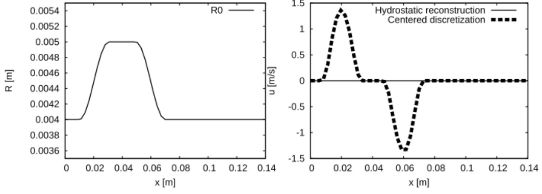
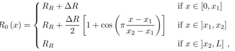
Here we describe a strategy based on a local subsonic steady state reconstruction that allows one to derive a subsonic-well-balanced scheme, preserving exactly all the subsonic

Two major novelties are considered: (i) the diffusion law relating the flux of sediments and the slope of the topography is now nonlinear and involves a p- Laplacian with p &gt; 2

Abstract The aim of this work is the extraction of tannic acid (TA) with two commercial nonionic surfactants, sep- arately: Lutensol ON 30 and Triton X-114 (TX-114).The