HAL Id: hal-00107462
https://hal.archives-ouvertes.fr/hal-00107462
Submitted on 18 Oct 2006HAL is a multi-disciplinary open access archive for the deposit and dissemination of sci-entific research documents, whether they are pub-lished or not. The documents may come from
L’archive ouverte pluridisciplinaire HAL, est destinée au dépôt et à la diffusion de documents scientifiques de niveau recherche, publiés ou non, émanant des établissements d’enseignement et de
Batch and median neural gas
Marie Cottrell, Barbara Hammer, Alexander Hasenfuss, Thomas Villmann
To cite this version:
Marie Cottrell, Barbara Hammer, Alexander Hasenfuss, Thomas Villmann. Batch and median neural gas. Neural Networks, Elsevier, 2006, 19, pp.762-771. �10.1016/j.neunet.2006.05.018�. �hal-00107462�
ccsd-00107462, version 1 - 18 Oct 2006
Batch and median neural gas
Marie Cottrell
SAMOS-MATISSE, Universit´e Paris I, Paris, France
Barbara Hammer
1Institute of Computer Science, Clausthal University of Technology, Clausthal-Zellerfeld, Germany
Alexander Hasenfuß
Institute of Computer Science, Clausthal University of Technology, Clausthal-Zellerfeld, Germany
Thomas Villmann
Clinic for Psychotherapy, Universit¨at Leipzig, Leipzig, Germany
1 corresponding author: Barbara Hammer, Institute of Computer Science, Clausthal
University of Technology, Julius-Albert-Str. 4, D-38678 Clausthal-Zellerfeld, Germany, [email protected]
Abstract
Neural Gas (NG) constitutes a very robust clustering algorithm given euclidian data which does not suffer from the problem of local minima like simple vector quantization, or topo-logical restrictions like the self-organizing map. Based on the cost function of NG, we introduce a batch variant of NG which shows much faster convergence and which can be interpreted as an optimization of the cost function by the Newton method. This formulation has the additional benefit that, based on the notion of the generalized median in analogy to Median SOM, a variant for non-vectorial proximity data can be introduced. We prove con-vergence of batch and median versions of NG, SOM, and k-means in a unified formulation, and we investigate the behavior of the algorithms in several experiments.
Key words: Neural gas, batch algorithm, proximity data, median-clustering, convergence
1 Introduction
Clustering constitutes a fundamental problem in various areas of applications such as pattern recognition, image processing, data mining, data compression, or ma-chine learning [23]. The goal of clustering is grouping given training data into classes of similar objects such that data points with similar semantical meaning are linked together. Clustering methods differ in various aspects including the assign-ment of data points to classes which might be crisp or fuzzy, the arrangeassign-ment of clusters which might be flat or hierarchical, or the representation of clusters which might be represented by the collection of data points assigned to a given class or by few prototypical vectors. In this article, we are interested in neural clustering algo-rithms which deal with crisp assignments and representation of clusters by neurons
or prototypes.
Popular neural algorithms representing data by a small number of typical proto-types include k-means, the self-organizing map (SOM), neural gas (NG), and al-ternatives [11,27]. Depending on the task and model at hand, these methods can be used for data compression, data mining and visualization, nonlinear projection and interpolation, or preprocessing for supervised learning. K-means clustering directly aims at a minimization of the quantization error [5]. However, its update scheme is local, therefore it easily gets stuck in local optima. Neighborhood cooperation as for SOM and NG offers one biologically plausible solution. Apart from a reduction of the influence of initialization, additional semantical insight is gained: browsing within the map and, if a prior low dimensional lattice is chosen, data visualization become possible. However, a fixed prior lattice as chosen in SOM might be subop-timal for a given task depending on the data topology and topological mismatches can easily occur [30]. SOM does not possess a cost function in the continuous case, and the mathematical analysis is quite difficult unless variations of the origi-nal learning rule are considered for which cost functions can be found [9,16]. NG optimizes a cost function which, as a limit case, yields the quantization error [21]. Thereby, a data optimum (irregular) lattice can be determined automatically dur-ing traindur-ing which perfectly mirrors the data topology and which allows to browse within the result [22]. This yields very robust clustering behavior. Due to the po-tentially irregular lattice, visualization requires additional projection methods.
These neural algorithms (or a variation thereof for SOM) optimize some form of cost function connected to the quantization error of the data set. There exist mainly two different optimization schemes for these objectives: online variants, which adapt the prototypes after each pattern, and batch variants which adapt the
pro-totypes according to all patterns at once. Batch approaches are usually much faster in particular for high dimensional vectors, since only one adaptation is necessary in each cycle and convergence can usually be observed after few steps. However, the problem of local optima for k-means remains in the batch variant. For SOM, topo-logical ordering might be very difficult to achieve since, at the beginning, ordering does usually not exist and, once settled in a topological mismatch, the topology can hardly be corrected. The problem of topological mismatches is much more pro-nounced in Batch SOM than in online SOM as shown in [12] such that a good (and possibly costly) initialization is essential for the success. However, due to their ef-ficiency, batch variants are often chosen for SOM or k-means if data are available a priori, whereby the existence of local optima and topological mismatches might cause severe problems. For NG, some variants of batch adaptation schemes oc-cur at singular points in the literature [32], however, so far, no NG-batch scheme has been explicitely derived from the NG cost function together with a proof of the convergence of the algorithm. In this article, we put the cost functions of NG, (modified) SOM, and k-means into a uniform notation and derive batch versions thereof together with a proof for convergence. In addition, we relate Batch NG to an optimization by means of the Newton method, and we compare the methods on different representative clustering problems.
In a variety of tasks such as classification of protein structures, text documents, surveys, or biological signals, an explicit metric vector space such as the standard euclidian vector space is not available, rather discrete transformations of data e.g. the edit distance or pairwise proximities are available [10,13,28]. In such cases, a clustering method which does not rely on a vector space has to be applied such as spectral clustering [2]. Several alternatives to SOM have been proposed which can deal with more general, mostly discrete data [10,13,28]. The article [19]
pro-poses a particularly simple and intuitive possibility for clustering proximity data: the mean value of the Batch SOM is substituted by the generalized median result-ing in Median SOM, a prototype-based neural network in which prototypes loca-tion are adapted within the data space by batch computaloca-tions. Naturally, the same idea can be transferred to Batch NG and k-means as we will demonstrate in this contribution. As for the euclidian versions, it can be shown that the median vari-ants of SOM, NG, and k-means converge after a finite number of adaptation steps. Thus, the formulation of neural clustering schemes by means of batch adaptation opens the way towards the important field of clustering complex data structures for which pairwise proximities or a kernel matrix constitute the interface to the neural clustering method.
2 Neural gas
Assume data points~x ∈ Rm are distributed according to an underlying distribution P , the goal of NG as introduced in [21] is to find prototype locations ~wi ∈ Rm, i = 1, . . . , n, such that these prototypes represent the distribution P as accurately as possible, minimizing the cost function
ENG( ~w) = 1 2C(λ) n X i=1 Z hλ(ki(~x, ~w)) · d(~x, ~wi) P (d~x) where d(~x, ~y) = (~x − ~y)2 denotes the squared euclidian distance,
is the rank of the prototypes sorted according to the distances,hλ(t) = exp(−t/λ) is a Gaussian shaped curve with neighborhood rangeλ > 0, and C(λ) is the con-stantPni=1hλ(ki). The learning rule consists of a stochastic gradient descent, yield-ing
∆ ~wi = ǫ · hλ(ki(~xj, ~w)) · (~xj− ~wi)
for all prototypesw~i given a data point~xj. Thereby, the neighborhood range λ is decreased during training to ensure independence of initialization at the beginning of training and optimization of the quantization error in the final stages. As pointed out in [22], the result can be associated with a data optimum lattice such that brows-ing within the data space constitutes an additional feature of the solution.
Due to its simple adaptation rule, the independence of a prior lattice, and the inde-pendence of initialization because of the integrated neighborhood cooperation, NG is a simple and highly effective algorithm for data clustering. Popular alternative clustering algorithms are offered by the SOM as introduced by Kohonen [18] and k-means clustering [11].
SOM uses the adaptation strengthhλ(nd (I(~xj), i)) instead of hλ(ki(~xj, ~w)), I(~xj) denoting the index of the closest prototype, the winner, for~xj, and nd a priorly cho-sen, often two-dimensional neighborhood structure of the neurons. A low-dimensional lattice offers the possibility to easily visualize data. However, if the primary goal is clustering, a fixed topology puts restrictions on the map and topology preservation often cannot be achieved [30]. SOM does not possess a cost function in the continu-ous case and its mathematical investigation is difficult [9]. However, if the winner is chosen as the neuroni with minimum averaged distancePn
l=1hλ(nd (i, l))d(~xj, ~wl), it optimizes the cost
ESOM( ~w) ∼ n X i=1 Z χI∗(~x)(i) · n X l=1 hλ(nd (i, l)) · d(~x, ~wl) P (d~x)
as pointed out by Heskes [16]. Here,I∗(~x) denotes the winner index according to the averaged distance andχj(i) is the characteristic function of j.
K-means clustering adapts only the winner in each step, thus it optimizes the stan-dard quantization error
Ekmeans( ~w) ∼ n X i=1 Z χI(~x)(i) · d(~x, ~wi) P (d~x)
whereI(~x) denotes the winner index for ~x in the classical sense. Unlike SOM and NG, k-means is very sensitive to initialization of the prototypes since it adapts the prototypes only locally according to their nearest data points. An initialization of the prototypes within the data points is therefore mandatory.
2.1 Batch clustering
If training data~x1, . . . ,~xp are given priorly, fast alternative batch training schemes exist for both, k-means and SOM. Starting from random positions of the prototypes, batch learning iteratively performs the following two steps until convergence
(1) determine the winnerI(~xi) resp. I∗(~xi) for each data point ~xi, (2) determine new prototypes as
~
wi = X j| I(~xj)=i
~xj/|{j | I(~xj) = i}|
for k-means and
~ wi = p X j=1 hλ(nd (I∗(~xj), i)) · ~xj/ p X j=1 hλ(nd (I∗(~xj), i)) for SOM.
Thereby, the neighborhood cooperation is annealed for SOM in the same way as in the online case.
It has been shown in [5,7] that Batch k-means and Batch SOM optimize the same cost functions as their online variants, whereby the modified winner notation as proposed by Heskes is used for SOM. In addition, as pointed out in [16], this formu-lation allows to link the models to statistical formuformu-lations and it can be interpreted as a limit case of EM optimization schemes for appropriate mixture models.
Often, batch training converges after only few (10-100) cycles such that this train-ing mode offers considerable speedup in comparison to the online variants: adap-tation of the (possibly high dimensional) prototypes is only necessary after the presentation of all training patterns instead of each single one.
Here, we introduce Batch NG. As for SOM and k-means, it can be derived from the cost function of NG, which, for discrete data~x1, . . . ,~xp, reads as
ENG( ~w) ∼ n X i=1 p X j=1 hλ(ki(~xj, ~w)) · d(~xj, ~wi) ,
d being the standard euclidian metric. For the batch algorithm, the quantities kij := ki(~xj, ~w) are treated as hidden variables with the constraint that the values kij (i = 1, . . . , n) constitute a permutation of {0, . . . , n − 1} for each point ~xj.ENG is interpreted as a function depending onw and k~ ij which is optimized in turn with respect to the hidden variableskij and with respect to the prototypes w~i, yielding the two adaptation steps of Batch NG which are iterated until convergence:
(1) determine
kij = ki(~xj, ~w) = |{ ~wl| d(~xj, ~wl) < d(~xj, ~wi)}| as the rank of prototypew~i,
(2) based on the hidden variableskij, set ~ wi = Pp j=1hλ(kij) · ~xj Pp j=1hλ(kij) .
As for Batch SOM and k-means, adaptation takes place only after the presentation of all patterns with a step size which is optimized by means of the partial cost func-tion. Only few adaptation steps are usually necessary due to the fact that Batch NG can be interpreted as Newton optimization method which takes second order infor-mation into account whereas online NG is given by a simple stochastic gradient descent.
To show this claim, we formulate the Batch NG update in the form
∆ ~wi = Pp j=1hλ(kij) · (~xj− ~wi) Pp j=1hλ(kij) .
Newton’s method for an optimization ofENGyields the formula
△ ~wi
= −J( ~wi
) · H−1( ~wi) ,
whereJ denotes the Jacobian of ENGandH the Hessian matrix. Since kijis locally constant, we get up to sets of measure zero
J( ~wi ) = 2 · p X j=1 hλ(kij) · ( ~wi− ~xj)
and the Hessian matrix equals a diagonal matrix with entries
2 · p X j=1
hλ(kij) .
The inverse gives the scaling factor of the Batch NG adaptation, i.e. Batch NG equals Newton’s method for the optimization ofENG.
2.2 Median clustering
Before turning to the problem of clustering proximity data, we formulate Batch NG, SOM, and k-means within a common cost function. In the discrete setting, these three models optimize a cost function of the form
E := n X i=1 p X j=1 f1(kij( ~w)) · f2ij( ~w)
where f1(kij( ~w)) is the characteristic function of the winner, i.e. χI(~xj)(i) resp.
χI∗(~xj)(i), for k-means and SOM, and it is hλ(ki(~xj, ~w)) for neural gas. f2ij( ~w)
equals the distance d(~xi, ~wj) for k-means and NG, and it is the averaged dis-tancePnl=1hλ(nd (i, l)) · d(~xj, ~wl) for SOM. The batch algorithms optimize E with respect to kij in step (1) assuming fixed w. Thereby, for each j, the vector k~ ij (i = 1, . . . , n) is restricted to a vector with exactly one entry 1 and 0, otherwise, for k-means and SOM. It is restricted to a permutation of{0, . . . , n − 1} for NG. Thus, the elements kij come from a discrete set which we denote by K. In step
(2),E is optimized with respect to ~wj assuming fixed k
ij. The update formulas as introduced above can be derived by taking the derivative off2ij with respect tow.~
For proximity data~x1, . . . ,~xp, only the distance matrixd
ij := d(~xi, ~xj) is available but data are not embedded in a vector space and no continuous adaptation is possi-ble, nor does the derivative of the distance functiond exist. A solution to tackle this setting with SOM-like learning algorithms proposed by Kohonen is offered by the Median SOM: it is based on the notion of the generalized median [19]. Prototypes are chosen from the discrete set given by the training pointsX = {~x1, . . . , ~xp} in an optimum way. In mathematical terms, E is optimized within the set Xngiven
by the training data instead of(Rm)n. This leads to the choice ofw~i as ~ wi = ~xl where l = argminl′ p X j=1 hλ(nd (I∗(~xj), i)) · d(~xj, ~xl ′ )
in step (2). In [19], Kohonen considers only the data points mapped to a neighbor-hood of neuroni as potential candidates for ~wi and, in addition, reduces the above sum to points mapped into a neighborhood of i. For small neighborhood range and approximately ordered maps, this does not change the result but considerably speeds up the computation.
The same principle can be applied to k-means and Batch NG. In step (2), instead of taking the vectors in(Rm)nwhich minimizeE, prototype i is chosen as the data point inX with ~ wi = ~xl where l = argminl′ p X j=1 χI(~xj)(l) · d(~xj, ~xl ′ ) assuming fixedχI(~xj)(l) for Median k-means and
~ wi = ~xl where l = argminl′ p X j=1 hλ(kij) · d(~xj, ~xl ′ )
assuming fixed kij = ki(~xj, ~w) for Median NG. For roughly ordered maps, a re-striction of potential candidates ~xl to data points mapped to a neighborhood of i can speed up training as for Median SOM.
Obviously, a direct implementation of the new prototype locations requires time
O(p2n), p being the number of patterns and n being the number of neurons, since for every prototype and every possible prototype location inX a sum of p terms needs to be evaluated. Hence, an implementation of Median NG requires the com-plexity O(p2n + pn log n) for each cycle, including the computation of k
ij for ev-eryi and j. For Median SOM, a possibility to speed up training has recently been presented in [8] which yields an exact computation with costs only O(p2 + pn2)
instead of O(p2n) for the sum. Unfortunately, the same technique does not improve the complexity of NG. However, further heuristic possibilities to speed-up median-training are discussed in [8] which can be transferred to Median NG. In particular, the fact that data and prototype assignments are in large parts identical for consec-utive runs at late stages of training and a restriction to candidate median points in the neighborhood of the previous one allows a reuse of already computed values and a considerable speedup.
2.3 Convergence
All batch algorithms optimizeE = E( ~w) by consecutive optimization of the hid-den variableskij( ~w) and ~w. We can assume that, for given ~w, the values kij deter-mined by the above algorithms are unique, introducing some order in case of ties. Note that the valueskij come from a discrete setK. If the values kij are fixed, the choice of the optimum w is unique in the algorithms for the continuous case, as~ is obvious from the formulas given above, and we can assume uniqueness for the median variants by introducing an order. Consider the function
Q( ~w′, ~w) = n X i=1 p X j=1 f1(kij( ~w)) · f ij 2 ( ~w′) .
Note thatE( ~w) = Q( ~w, ~w). Assume prototypes ~w are given, and new prototypes ~w′ are computed based onkij( ~w) using one of the above batch or median algorithms. It holdsE( ~w′) = Q( ~w′, ~w′) ≤ Q( ~w′, ~w) because k
ij( ~w′) are optimum assignments for kij in E, given ~w′. In addition, Q( ~w′, ~w) ≤ Q( ~w, ~w) = E( ~w) because ~w′ are optimum assignments of the prototypes givenkij( ~w). Thus, E( ~w′) − E( ~w) = E( ~w′) − Q( ~w′, ~w) + Q( ~w′, ~w) − E( ~w) ≤ 0, i.e., in each step of the algorithms, E is decreased. Since there exists only a finite number of different valueskij and the
assignments are unique, the algorithms converge in a finite number of steps toward a fixed pointw~∗for which( ~w∗)′ = ~w∗holds.
Consider the case of continuous w. Since k~ ij are discrete,kij( ~w) is constant in a vicinity of a fixed point w~∗ if no data points lie at the borders of two receptive fields. Then E(·) and Q(·, ~w∗) are identical in a neighborhood of ~w∗ and thus, a local optimum ofQ is also a local optimum of E. Therefore, if ~w can be varied in a real vector space, a local optimum ofE is found by the batch variant if no data points are directly located at the borders of receptive fields for the final solution.
3 Experiments
We demonstrate the behavior of the algorithms in different scenarios which cover a variety of characteristic situations. All algorithms have been implemented based on the SOM Toolbox for Matlab [24]. We used k-means, SOM, Batch SOM, and NG with default parameters as provided in the toolbox. Batch NG and median versions of NG, SOM, and k-means have been implemented according to the above formulas. Note that, for all batch versions, prototypes which lie at identical points of the data space do not separate in consecutive runs. Thus, the situation of exactly identical prototypes must be avoided. For the euclidian versions, this situation is a set of measure zero if prototypes are initialized at different positions. For median versions, however, it can easily happen that prototypes become identical due to a limited number of different positions in the data space, in particular for small data sets. Due to this fact, we add a small amount of noise to the distances in each epoch in order to separate identical prototypes. Vectorial training sets are normalized prior to training using z-transformation. Initialization of prototypes takes place using small random values. The initial neighborhood rate for neural gas isλ = n/2, n
5 10 15 20 25 0 0.2 0.4 0.6 0.8 1 1.2 1.4
Quantization error on (normalized) 2D synthetic data
number of neurons NeuralGas BatchNeuralGas MedianNeuralGas kMeans MediankMeans 5 10 15 20 25 2 4 6 8 10 12 14 16
Quantization error on (normalized) segmentation data
number of neurons NeuralGas BatchNeuralGas MedianNeuralGas Som BatchSom MedianSom kMeans MediankMeans
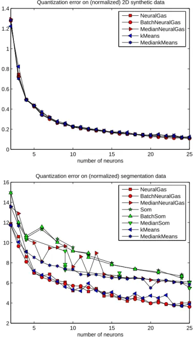
Fig. 1. Mean quantization error of the methods for the synthetic data set (top) and the segmentation data set (bottom).
being the number of neurons, and it is multiplicatively decreased during training. For Median SOM, we restrict to square lattices of n = √n × √n neurons and a rectangular neighborhood structure, whereby√n is rounded to the next integer. Here the initial neighborhood rate is√n/2.
−2.5 −2 −1.5 −1 −0.5 0 0.5 1 1.5 2 −3 −2 −1 0 1 2 3
Location of prototypes (6) for 2D synthetic data
NeuralGas BatchNeuralGas MedianNeuralGas −2.5 −2 −1.5 −1 −0.5 0 0.5 1 1.5 2 −3 −2 −1 0 1 2 3
Location of prototypes (12) for 2D synthetic data
NeuralGas BatchNeuralGas MedianNeuralGas
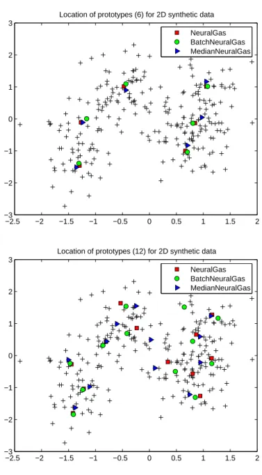
Fig. 2. Location of the prototypes for the synthetic data set for different variants of NG.
3.1 Synthetic data
The first data set is the two-dimensional synthetic data set from [27] consisting of 250 data points and 1000 training points. Clustering has been done using n = 2, . . . , 25 prototypes, resp. the closest number of prototypes implemented by a rectangular lattice for SOM. Training takes place for5n epochs.
The mean quantization error Pni=1Ppj=1χI(~xj)(i) · d(~xj, ~wi)/p on the test set and
the location of prototypes within the training set are depicted in Figs. 1 and 2. Obviously, the location of prototypes coincides for different versions of NG. This observation also holds for different numbers of prototypes, whereby the result is subject to random fluctuations for larger numbers. For k-means, idle prototypes can be observed for largen. For Batch SOM and standard SOM, the quantization error is worse (ranging from1.7 for 2 neurons up to 0.3 for 24 neurons, not depicted in the diagram), which can be attributed to the fact that the map does not fully unfold upon the data set and edge effects remain, which could be addressed to a small but nonvanishing neighborhood in the convergent phase in standard implementations of SOM which is necessary to preserve topological order. Median SOM (which has been directly implemented in analogy to Median NG) yields a quantization error competitive to NG. Thus, Batch and Median NG allow to achieve results competitive to NG in this case, however, using less effort.
3.2 Segmentation data
The segmentation data set from the UCI repository consists of 210 (training set) resp.2100 (test set) 19 dimensional data points which are obtained as pixels from outdoor images preprocessed by standard filters such as averaging, saturation, in-tensity, etc. The problem is interesting since it contains high dimensional and only sparsely covered data. The quantization error obtained for the test set is depicted in Fig. 1. As beforehand, SOM suffers from the restriction of the topology. Neural gas yields very robust behavior, whereas for k-means, idle prototypes can be observed. The median versions yield a larger quantization error compared to the vector-based algorithms. The reason lies in the fact that a high dimensional data set with only few
training patterns is considered, such that the search space for median algorithms is small in these cases and random effects and restrictions account for the increased error.
3.3 Checkerboard
This data set is taken from [15]. Two-dimensional data are arranged on a checker-board, resulting in10 times 10 clusters, each consisting of 15 to 20 points. For each algorithm, we train5 times 100 epochs for 100 prototypes. Obviously, the problem is highly multimodal and usually the algorithms do not find all clusters. The num-ber of missed clusters can easily be judged in the following way: the clusters are
NG batch median SOM batch median kmeans median
NG NG SOM SOM kmeans
quantization error train 0.0043 0.0028 0.0043 0.0127 0.0126 0.0040 0.0043 0.0046 test 0.0051 0.0033 0.0048 0.0125 0.0124 0.0043 0.0050 0.0052 classification error train 0.1032 0.0330 0.0338 0.2744 0.2770 0.0088 0.1136 0.0464 test 0.1207 0.0426 0.0473 0.2944 0.2926 0.0111 0.1376 0.0606 Table 1
Quantization error and classification error for posterior labeling for training and test set (both are of size about 1800). The mean over 5 runs is reported. The best results on the test set is depicted in boldface.
labeled consecutively using labels1 and 2 according to the color black resp. white of the data on the corresponding field of the checkerboard. We can assign labels to prototypes a posteriori based on a majority vote on the training set. The num-ber of errors which arise from this classification on an independent test set count the number of missed clusters, since1% error roughly corresponds to one missed cluster.
The results are collected in Tab. 1. The smallest quantization error is obtained by Batch NG, the smallest classification error can be found for Median SOM. As be-forehand, the implementations for SOM and Batch SOM do not fully unfold the map among the data. In the same way online NG does not achieve a small error because of a restricted number of epochs and a large data set which prevents online NG from full unfolding. K-means also shows a quite high error (it misses more than10 clusters) which can be explained by the existence of multiple local optima in this setting, i.e. the sensitivity of k-means with respect to initialization of proto-types. In contrast, Batch NG and Median NG find all but3 to 4 clusters. Median SOM even finds all but only1 or 2 clusters since the topology of the checkerboard exactly matches the underlying data topology consisting of10 × 10 clusters. Sur-prisingly, also Median k-means shows quite good behavior, unlike k-means itself, which might be due to the fact that the generalized medians enforce the prototypes to settle within the clusters. Thus, median versions and neighborhood cooperation seem beneficial in this task due to the multiple modes. Batch versions show much better behavior than their online correspondents, due to a faster convergence of the algorithms. Here, SOM suffers from border effects, whereas Median SOM settles within the data clusters, whereby the topology mirrors precisely the data topology. Both, Batch NG and Median NG, yield quite good classification results which are even competitive to supervised prototype-based classification results as reported in
20 40 60 80 100 120 140 20 40 60 80 100 120 140
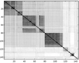
Fig. 3. Distance matrix for protein data.
[15].
3.4 Proximity data – protein clusters
We used the protein data set described in [29] and [28]: the dissimilarity of 145 globin proteins of different families is given in matrix form as depicted in Fig. 3. Thereby, the matrix is determined based on sequence alignment using biochemical and structural information. In addition, prior information about the underlying pro-tein families is available, i.e. a prior clustering into semantically meaningful classes of the proteins is known: as depicted in Fig 4 by vertical lines, the first 42 proteins belong to hemoglobinα, the next clusters denote hemoglobin β, δ, etc. Thereby, several clusters are rather small, comprising only few proteins (one or two). In ad-dition, the cluster depicted on the right has a very large intercluster distance.
Since only a proximity matrix is available, we cannot apply standard NG, k-means, or SOM, but we can rely on the median versions. We train all three median versions 10 times using 10 prototypes and 500 epochs. The mean quantization errors (and
variances) are3.7151 (0.0032) for Median NG 3.7236 (0.0026) for Median SOM, and4.5450 (0.0) for Median k-means, thus k-means yields worse results compared to NG and SOM and neighborhood integration clearly seems beneficial in this ap-plication scenario.
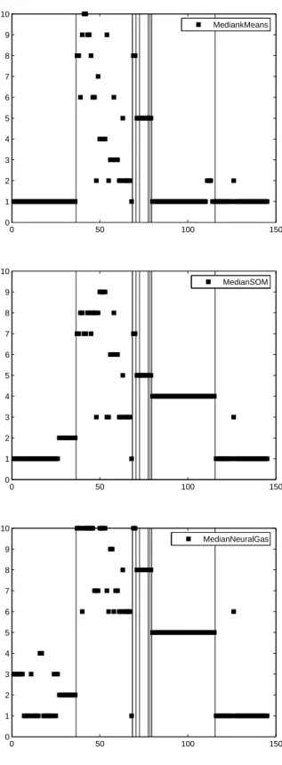
We can check whether the decomposition into clusters by means of the prototypes is meaningful by comparing the receptive fields of the ten prototypes to the prior semantic clustering. Typical results are depicted in Fig. 4. The classification pro-vided by experts is indicated by vertical lines in the images. The classification by the respective median method is indicated by assigning a value on the y-achses to each pattern corresponding to the number of its winner neuron (black squares in the figure). Thus, an assignment of all or nearly all patterns in one semantic cluster to one or few dedicated prototypes gives a hint for the fact that median clustering finds semantically meaningful entities.
All methods detect the first cluster (hemoglobinα) and neural gas and SOM also detect the eighth cluster (myoglobin). In addition, SOM and NG group together elements of clusters two to seven in a reasonable way. Thereby, according to the variance in the clusters, more than one prototype is used for large clusters and small clusters containing only one or two patterns are grouped together. The elements of the last two clusters have a large intercluster distance such that they are grouped together into some (random) cluster for all methods. Note that the goal of NG and SOM is a minimization of their underlying cost function, such that the cluster bor-der can lie between semantic clusters for these methods. Thus, the results obtained by SOM and NG are reasonable and they detect several semantically meaningful clusters. The formation of relevant clusters is also supported when training with a different number of prototypes
3.5 Proximity data – chicken pieces silhouettes
The data set as given in [1] consists of silhouettes of446 chicken pieces of different classes including wings, backs, drumsticks, thighs, and breasts. The task is a clas-sification of the images (whereby the silhouettes are not oriented) into the correct class. As described in [26], a preprocessing of the images resulting in a proximity matrix can cope with the relevant properties of the silhouette and rotation symme-try: the surrounding edges are detected and discretized into small consecutive line segments of20 pixels per segment. The images are then represented by the differ-ences of the angles of consecutive line segments. Distance computation takes place as described in [6] by a rotation and mirror symmetric variant of the edit distance of two sequences of angles, whereby the costs for a substitution of two angles is given by their absolute distance, the costs for deletion and insertion are given by k = 60.
We train Median k-means, Median NG, and Median SOM with different numbers of neurons for500 epochs, thereby annealing the neighborhood as beforehand. The results on a training and test set of the same size, averaged over ten runs, are de-picted in Tab. 2. Obviously, a posterior labeling of prototypes obtained by median clustering allows to achieve a classification accuracy of more than 80%. Thereby, overfitting can be observed for all methods due to the large number of prototypes compared to the training set (50 neurons constitute about 1/4th of the training set!). However, Median NG and Median SOM are less prone to this effect due to their inherent regularization given by the neighborhood integration.
neurons Median k-means Median NG Median SOM
train test train test train test
10 0.54 0.52 0.57 0.61 0.53 0.59 20 0.71 0.61 0.67 0.65 0.61 0.61 30 0.77 0.63 0.73 0.64 0.69 0.61 40 0.85 0.79 0.80 0.75 0.74 0.69 50 0.90 0.79 0.84 0.80 0.76 0.68 60 0.88 0.82 0.88 0.83 0.80 0.73 70 0.93 0.82 0.89 0.84 0.89 0.78 80 0.94 0.82 0.92 0.84 0.87 0.78 90 0.95 0.81 0.93 0.84 0.87 0.78 100 0.96 0.83 0.94 0.83 0.88 0.80 Table 2
Results for the median variants for different numbers of neurons on the chicken-piece-silhouettes data base. The best test classifications are depicted in bold.
3.6 Proximity data – chromosomes
The Copenhagen Chromosomes Database [20] consists of 4400 descriptions of chromosomes by their silhouettes in images. A chromosome is described by a se-quence over the alphabet{1, . . . , 6}, whereby the number describes the thickness of the density profile of the protein at the corresponding position. The difference between two profiles is determined by alignment assigning the costs |x − y| to
substitutions ofx and y, and assigning the costs 4.5 to insertions and deletions, as described in [26]. There are21 different classes. The set is divided into a training and test set of the same size.
We train median clustering with different numbers of neurons and100 cycles. The classification accuracy on a training and test set, averaged over10 runs, is depicted in Tab. 3. As beforehand, a classification accuracy of80% can be achieved. Thereby, Median NG shows the best results on the test set for almost all numbers of neurons, accompanied by a good generalization error due to the inherent regularization by means of neighborhood cooperation.
4 Conclusions
We have proposed Batch NG derived from the NG cost function which allows fast training for a priorly given data set. We have shown that the method converges and it optimizes the same cost function as NG by means of a Newton method. In addition, the batch formulation opens the way towards general proximity data by means of the generalized median. These theoretical discussions were supported by experiments for different vectorial data where the results of Batch NG and NG are very similar. In all settings, the quality of Batch NG was at least competitive to standard NG, whereby training takes place in a fraction of the time especially for high-dimensional input data due to the radically reduced number of updates of a prototype. Unlike k-means, NG is not sensitive to initialization and, unlike SOM, it automatically determines a data optimum lattice, such that a small quantization error can be achieved and topological initialization is not crucial.
neurons Median k-means Median NG Median SOM
train test train test train test
10 0.31 0.25 0.43 0.40 0.40 0.34 20 0.52 0.45 0.46 0.42 0.54 0.52 30 0.64 0.57 0.70 0.66 0.57 0.53 40 0.75 0.62 0.75 0.71 0.69 0.63 50 0.78 0.73 0.79 0.74 0.75 0.67 60 0.80 0.74 0.83 0.78 0.75 0.67 70 0.75 0.68 0.82 0.77 0.69 0.60 80 0.82 0.75 0.83 0.78 0.68 0.58 90 0.82 0.74 0.82 0.76 0.73 0.65 100 0.82 0.76 0.86 0.81 0.78 0.72 Table 3
Classification accuracy on the chromosome data set for different numbers of neurons. The best results on the test set are depicted in bold.
can be applied to non-vectorial data. We compared Median NG to its alternatives for vectorial data observing that competitive results arise if enough data are avail-able. We added several experiments including proximity data where we could ob-tain semantically meaningful grouping as demonstrated by a comparison to known clusters resp. a validation of the classification error when used in conjunction with posterior labeling. Unlike SOM, NG solely aims at data clustering and not data vi-sualization, such that it can use a data optimum lattice and it is not restricted by
topological constraints. Therefore better results can often be obtained in terms of the quantization error or classification. If a visualization of the output of NG is desired, a subsequent visualization of the prototype vectors is possible using fast standard methods for the reduced set of prototypes such as multidimensional scal-ing [4].
Thus, very promising results could be achieved which have been accompanied by mathematical guarantees for the convergence of the algorithms. Nevertheless, sev-eral issues remain: for sparsely covered data sets, median versions might not have enough flexibility to position the prototypes since only few locations in the data space are available. We have already demonstrated this effect by a comparison of batch clustering to standard euclidian clustering in such a situation. It might be worth investigating metric-specific possibilities to extend the adaptation space for the prototypes in such situations, as possible e.g. for the edit distance, as demon-strated in [14] and [25].
A problem of Median NG is given by the complexity of one cycle, which is quadratic in the number of patterns. Since optimization of the exact computation as proposed in [8] is not possible, heuristic variants which restrict the computation to regions close to the winner seem particularly promising because they have a minor effect on the outcome. A thorough investigation of the effects of such restriction will be investigated both theoretically and experimentally in future work.
Often, an appropriate metric or proximity matrix is not fully known a priori. The technique of learning metrics, which has been developed for both, supervised as well as unsupervised prototype-based methods [15,17] allows a principled inte-gration of secondary knowledge into the framework and adapts the metric accord-ingly, thus getting around the often problematic ‘garbage-in-garbage-out’ problem
of metric-based approaches. It would be interesting to investigate the possibility to enhance median versions for proximity data by an automatic adaptation of the dis-tance matrix during training driven by secondary information. A recent possibility to combine vector quantizers with prior (potentially fuzzy) label information has been proposed in [31] by means of a straightforward extension of the underlying cost function of NG. This approach can immediately be transferred to a median computation scheme since a well-defined cost function is available, thus opening the way towards supervised prototype-based median fuzzy classification for non-vectorial data. A visualization driven by secondary label information can be de-veloped within the same framework substituting the irregular NG lattice by a SOM neighborhood and incorporating Heskes’ cost function. An experimental evaluation of this framework is the subject of ongoing work.
References
[1] G. Andreu, A. Crespo, and J.M. Valiente (1997), Selecting the toroidal self-organizing feature maps (TSOFM) best organized to object recognition, Proceedings of ICNN’97, 2:1341-1346.
[2] M. Belkin and P. Niyogi (2002), Laplacian eigenmaps and spectral techniques for embedding and clustering, NIPS 2001, 585-591, T.G. Dietterich, S. Becker, and Z. Ghahramani (eds.), MIT Press.
[3] C.L. Blake and C.J. Merz (1998), UCI Repository of machine learning databases, Irvine, CA, University of California, Department of Information and Computer Science.
[4] I. Borg and P. Groenen (1997), Modern multidimensional scaling: theory and applications, Springer.
[5] L. Bottou and Y. Bengio (1995), Convergence properties of the k-means algorithm, in
NIPS 1994, 585-592, G. Tesauro, D.S. Touretzky, and T.K. Leen (eds.), MIT.
[6] H. Bunke and U. B ¨uhler (1993), Applications of approximate string matching to 2D shape recognition. Pattern Recognition 26(12): 1797-1812.
[7] Y. Cheng (1997), Convergence and ordering of Kohonen’s batch map, Neural
Computation 9:1667-1676.
[8] B. Conan-Guez, F. Rossi, and A. El Golli (2005), A fast algorithm for the self-organizing map on dissimilarity data, in Workshop on Self-Organizing Maps, 561-568.
[9] M. Cottrell, J.C. Fort, and G. Pag`es (1999), Theoretical aspects of the SOM algorithm,
Neurocomputing 21:119-138.
[10] M. Cottrell, S. Ibbou, and P. Letr´emy (2004), SOM-based algorithms for qualitative variables, Neural Networks 17:1149-1168.
[11] R.O. Duda, P.E. Hart, and D.G. Storck (2000), Pattern Classification, Wiley.
[12] J.-C. Fort, P. Letr´emy, and M. Cottrell (2002), Advantages and drawbacks of the Batch Kohonen algorithm, in ESANN’2002, M. Verleysen (ed.), 223-230, D Facto.
[13] T. Graepel and K. Obermayer (1999), A self-organizing map for proximity data,
Neur.Comp. 11:139-155.
[14] S. Guenter and H. Bunke (2002), Self-organizing map for clustering in the graph domain, Pattern Recognition Letters 23: 401 - 417.
[15] B. Hammer, M. Strickert, and T. Villmann (2005), Supervised neural gas with general similarity measure, Neural Processing Letters 21:21-44.
[16] T. Heskes (2001), Self-organizing maps, vector quantization, and mixture modeling,
[17] S. Kaski and J. Sinkkonen (2004), Principle of learning metrics for data analysis,
Journal of VLSI Signal Processing, special issue on Machine Learning for Signal
Processing, 37: 177-188.
[18] T. Kohonen (1995), Self-Organizing Maps, Springer.
[19] T. Kohonen and P. Somervuo (2002), How to make large self-organizing maps for nonvectorial data, Neural Networks 15:945-952.
[20] C. Lundsteen, J. Phillip, and E. Granum (1980), Quantitative analysis of 6985 digitized trypsin G-banded human metaphase chromosomes, Clinical Genetics 18:355-370.
[21] T. Martinetz, S.G. Berkovich, and K.J. Schulten (1993), ‘Neural-gas’ network for vector quantization and its application to time-series prediction, IEEE Transactions
on Neural Networks 4:558-569.
[22] T. Martinetz and K.J. Schulten (1994), Topology representing networks, Neural
Networks 7:507-522.
[23] M.N. Murty, A.K. Jain, and P.J. Flynn (1999), Data clustering: a review, ACM
Computing Surveys 31:264-323.
[24] Neural Networks Research Centre, Helsinki University of Technology, SOM Toolbox, http://www.cis.hut.fi/projects/somtoolbox/
[25] P. Somervuo, Online Algorithm for the Self-Organizing Map of Symbol Strings (2004), Neural Networks 17: 1231-1239.
[26] B. Spillmann (2004), Description of distance matrices, University of Bern, http://www.iam.unibe.ch/∼fki/varia/distancematrix/
[27] B.D. Ripley (1996), Pattern Recognition and Neural Networks, Cambridge.
[28] S. Seo and K. Obermayer (2004), Self-organizing maps and clustering methods for matrix data, Neural Networks 17:1211-1230.
[29] H. Mevissen and M. Vingron (1996), Quantifying the local reliability of a sequence alignment, Protein Engineering 9:127-132.
[30] T. Villmann, R. Der, M. Herrmann, and T. Martinetz (1994), Topology preservation in self-organizing feature maps: exact definition and measurement, IEEE Transactions
on Neural Networks 2:256-266.
[31] T. Villmann, B. Hammer, F.-M. Schleif, and T. Geweniger (2005), Fuzzy labeled neural gas for fuzzy classification, in Workshop on Self-Organizing Maps, 283-290.
[32] S. Zhong and J. Ghosh (2003), A unified framework for model-based clustering,
0 50 100 150 0 1 2 3 4 5 6 7 8 9 10 MediankMeans 0 50 100 150 0 1 2 3 4 5 6 7 8 9 10 MedianSOM 0 50 100 150 0 1 2 3 4 5 6 7 8 9 10 MedianNeuralGas
Fig. 4. Typical results for median classification and 10 prototypes. The x-axes shows the protein number, the y-axes its winner neuron. The vertical lines indicate an expert clas-sification into different protein families (from left to right: hemoglobin α, β, δ, ǫ, γ, F,