HAL Id: hal-00499421
https://hal.archives-ouvertes.fr/hal-00499421
Submitted on 9 Jul 2010
HAL is a multi-disciplinary open access
archive for the deposit and dissemination of
sci-entific research documents, whether they are
pub-lished or not. The documents may come from
teaching and research institutions in France or
L’archive ouverte pluridisciplinaire HAL, est
destinée au dépôt et à la diffusion de documents
scientifiques de niveau recherche, publiés ou non,
émanant des établissements d’enseignement et de
recherche français ou étrangers, des laboratoires
Blind Channel Identification and Extraction of more
Sources than Sensors
Pierre Comon
To cite this version:
Pierre Comon. Blind Channel Identification and Extraction of more Sources than Sensors. Advanced
Signal Processing Algorithms, Architectures, and Implementations VIII, Jul 1998, San Diego, United
States. pp.2-13, �10.1117/12.325670�. �hal-00499421�
Blind channel identification
and extraction of more sources than sensors
P. Comon
ba aI3S–CNRS, Algorithmes/Euclide, 2000 route des Lucioles,
Sophia-Antipolis, F-06410 Biot, France
b
Eurecom Institute, Mobile Communications Dept, BP193,
F-06904 Sophia-Antipolis, France
ABSTRACT
It is often admitted that a static system with more inputs (sources) than outputs (sensors, or channels) cannot be blindlyidentified, that is, identified only from the observation of its outputs, and without any a priori knowledge on the source statistics but their independence. By resorting to High-Order Statistics, it turns out that static MIMO systems with fewer outputs than inputs can be identified, as demonstrated in the present paper.
The principle, already described in a recent rather theoretical paper, had not yet been applied to a concrete blind identification problem. Here, in order to demonstrate its feasibility, the procedure is detailed in the case of a 2-sensor 3-source mixture; a numerical algorithm is devised, that blindly identifies a 3-input 2-output mixture. Computer results show its behavior as a function of the data length when sources are QPSK-modulated signals, widely used in digital communications.
Then another algorithm is proposed to extract the 3 sources from the 2 observations, once the mixture has been identified. Contrary to the first algorithm, this one assumes that the sources have a known discrete distribution. Computer experiments are run in the case of three BPSK sources in presence of Gaussian noise.
SPIE Conf. Adv. Sig. Proc. VIII, San Diego, 22-24 July, 1998, pp.2–13
Keywords: High-Order Statistics (HOS), Source Separation, Downlink Communications, User Extraction, Cumu-lant Tensor, Binary Quantics, Multiway array, Independent Component Analysis (ICA), Multiple Inputs Multiple Outputs (MIMO) static linear systems
1. INTRODUCTION
The principles on which the blind identification algorithm is based are related to rather unknown and forbidding canonical decompositions of homogeneous polynomials. Some of these results need to be introduced comprehensively. But algebra has been kept to a minimum, and a tradeoff between compactness and readability of the notation has been sought.
1.1. Notation
Throughout this paper, boldface letters, like u, will denote single way arrays, i.e. vectors. Its dimension is the range of variation of its index. Capital letters, like G, will denote arrays with more than one way, i.e. matrices or many-way arrays. The order of an array will refer to the number of its ways. The entries of an array of order d are accessed via d indices, say i1..id, every index ia ranging from 1 to na. The integer na is one of the d dimensions of the array.
For instance, a matrix is a 2-way array (order 2), and has thus 2 dimensions. A product between two arrays can be done in several manners. It is convenient to define two particular products.
Given two arrays, A = {Aij..!} and B = {Bi!j!..!!} of orders dA and dB respectively, having the same first
dimension, define the contraction product as:
(A • B)j..!j!..!! =
n1
!
i=1
Aij..!Bij!..!!
This product yields an array of order dA+ dB− 2. Next, the outer product yields an array of order dA+ dB and is
simply defined as:
(A ◦ B)ij..! i!j!..!! = Aij..!Bi!j!..!!
Examples. (i) Rank-one matrices are of the form u◦ v. (ii) The usual product between two matrices would be written A B = AT• B. (iii) The scalar product between two vectors can be written u • v. In the remaining, (T) will stand for transposition, (∗) for complex conjugation, and (†) for transposition and conjugation (i.e. Hermitian transposition).
1.2. Array decomposition
Now imagine data samples are stored in a d−way array, {Gi j..!}. This array is decomposable1 if it is equal to the
outer product of d vectors: G = u ◦ v ◦ · · · ◦ w. A general array is a superposition of decomposable arrays, and a common problem in data analysis is precisely to determine those constituting factors.1,2 In order to fix the ideas,
let’s concentrate on the fourth order case, and consider the array {Gijk!}. The problem consists of finding a family
of vector quadruples, (t(p), u(p), v(p), w(p)), such that G = "ωp=1 t(p) ◦ u(p) ◦ v(p) ◦ w(p). Clearly, three of the four factors can be determined only up to a constant multiplicative factor. It is thus legitimate to assume that these vectors have unit norm, without restricting generality, so that the model to identify is eventually:
G =
ω
!
p=1
γ(p) t(p) ◦ u(p) ◦ v(p) ◦ w(p) (1)
where γ(p) are unknown scalars, 1 ≤ p ≤ ω, and ω is minimal. For the moment, we shall refer to this equation as the Canonical Decomposition (CAND) of G. Note that this problem deflates to the standard factor analysis in the case of 2-way arrays.3 In the latter case, it now well known that the minimal value of ω allowing such a canonical
decomposition equals the rank of the matrix, and that the factors can be obtained by Singular Value Decomposition (SVD). However, the uniqueness is obtained to the price of imposing the additional constraint of orthogonality among each of the 2 families of ω vectors. This constraint is not mandatory at higher orders,4as will be pointed out subsequently.
1.3. Motivation
The motivation to go to higher order arrays is three-fold. First, as just said, the uniqueness is obtained with the help of an arbitrary constraint of orthogonality at order 2. This constraint may not be in accordance with the actual structure of the data. Second, data are often arranged in many-way arrays; the reduction to a 2-way array represents a loss of information. Third, the number of factors that can be identified is limited to the rank of the data matrix, itself bounded by the smallest dimension. Yet, there may very well be more factors than the smallest dimension.
Another field in data analysis where CAND is useful is learning theory. More precisely, if a probability density function (pdf) needs to be computed from a finite set of data in dimension n, then the number of samples required to reach a given relative precision grows exponentially with n. In practice, this makes it impossible to estimate pdf’s in dimensions as small as 9 or 10.5 One solution consists of splitting first the data into two subspaces of smaller
dimension, so that the pdf rewrites as well as possible as f (u, v) ≈ g(u) h(v). In other words, the data are almost statistically independent in the two subspaces.6The number of samples required in each of the two subspaces is thus
smaller by several orders of magnitude.
Beside data analysis, there are a number of fields where CAND is very useful, including Radar,7 Acoustics,
Com-plexity,1 or Digital communications, and particularly in military applications such as interception and classification
of radiating sources. In fact, the estimation of the sources must be carried out blindly in many military applications, that is, with very few a priori knowledge on the expected sources. In the civil domain, mobile communications need channel identification or equalization, which is carried out with the help of known sequences, emitted with this purpose. Since a small part of the source signal is known, one often refers to semi-blind equalization8of the channel.
Constructive algorithms executing semi-blind equalization are based on principles of both blind and clear-sighted equalization, hence the interest in blind approaches. In these problems, the statistics of the data are put in a d−way array instead of the data themselves.
To be more explicit, assume the data are measured on n sensors, and that they satisfy the following n−channel linear model:
where the components of x (referred to as sources) are statistically independent, and where A is a n × ω unknown full rank matrix. The problem of estimating the sources from measurements of y, solely based on independence between the xi’s is addressed in the literature under the terminology of Independent Component Analysis (ICA).9,10 It may
or may not conduct a prior blind identification of the mixing matrix A. In the former instance, it can be seen as a symmetric version of CAND. In the framework of ICA, the originality of the present work lies in the fact that the number of sources, ω, may be larger than the number of sensors, n. Let’s now be more explicit.
Random variables xi are statistically independent if all their cross-cumulants vanish.11 For instance, at order 4,
we should have that:
Cum{xi, xj, xk, x!} = γ(i) δ(i, j, k, $)
where δ is the Kronecker function, equal to 1 if all its arguments are equal and null otherwise. Yet, cumulants satisfy the multilinearity property,11 so that (2) implies that:
Gijk!=
!
p
γ(p) AipAjpAkpA!p (3)
if G denotes the fourth order cumulant tensor of y. Now denoting by a(p) the pth column of A, it is easily seen that (3) can be written as a symmetric canonical decomposition:
G =
ω
!
p=1
γ(p) a(p) ◦ a(p) ◦ a(p) ◦ a(p) (4)
This shows more explicitly that ICA is the symmetric version of CAND.
In the remaining, we shall be interested mainly in this symmetric decomposition, with d = 4, and with moderate values of the dimension n. In particular, in downlink mobile communications, it is realistic to assume that the receiver diversity will range between n = 2 and n = 4. In fact current equipment offers only n = 1, but it is reasonable to assume that n = 2 will be available in the near future, by exploiting either the spatial, sampling, or polarization diversities. In (4), n−dimensional vectors a(p) account for this diversity by the fact that they are not mutually collinear.
1.4. State of the art
In real world applications, it happens that the observation is dynamic, that is, y(t) = H(t)%x(t), where the mixture is characterized by a multichannel impulse response H(t) rather than by a constant matrix A. In such cases, additional equations can be utilized, as demonstrated by Tong12 or Regalia,13 even if ICA is underlying in all multichannel
blind equalization problems.14 But the problem with fewer sensors than sources has been very little addressed and
only very recently by the Signal Processing community, even in the static case (see for instance DeLathauwer15
Tong12Cao16 Comon4 et alterae).
In this paper, we concentrate only on the static model (2), also encountered in factor analysis. In the latter field, the problem started to raise serious attention around 1970 (see in particular Caroll17and Kruskal1). With the
terminology of this field, ω > n is translated into “more factors than subjects”.
Bergman18 has been probably the first to notice that the concept of rank is difficult to extend from matrices
to higher order arrays. Caroll17 provides the first canonical decomposition algorithm of a three-way array, later
referred to as Candecomp model. Kruskal1 conducts several years later a detailed analysis of uniqueness, and relates
several definitions of rank. The algorithm Candelinc2 was devised by Caroll and others in the eighties; it allows to
compute a canonical decomposition subject to a priori linear constraints. Leurgans19derives sufficient identifiability
conditions for the 3-way array decomposition; as opposed to Kruskal, his proof is constructive and yields a numerical algorithm running several matrix SVD’s. A solid account on decompositions of 3-way arrays can also be found in DeLathauwer’s PhD thesis15; an interesting tool defined therein is the HOSVD,20 generalizing the concept of SVD
to arrays of order 3, in a different manner compared to Caroll.
As shown in a recent work,4 symmetric arrays of order d and dimension n can be associated bijectively
to homogeneous polynomials of degree d in n variables. Based on this remark, decomposing a symmetric array is equivalent to decomposing a homogeneous polynomial into a sum of linear forms raised to the dth power (we shall go back to this in section 2). The advantage, compared to Candecomp, is that the symmetry is not broken. As a
consequence, the problem can then be connected to early works in invariant theory21and multilinear algebra.22The
first results go back to the beginning of the century with the works of Sylvester (see section 3.1) and Wakeford.23
One can also mention, among others, the works of Rota24 on binary quantics, and those of Reznick on quantics of
even degree,25especially in the complex case.26 Reznick introduced the concept of width, which corresponds to the
rank in the case of matrices.
2. POLYNOMIALS AND TENSOR ARRAYS
2.1. Linear spaces
A cumulant array may be considered as a tensor, because cumulants (as well as moments) satisfy the multilinearity property.11 For simplicity, tensors will be subsequently considered as mere arrays. The set of symmetric arrays of
order d and dimension n is a vector space of dimension:4
D(n; d) = # n + d − 1 d $ (5)
Now, every symmetric array G of order d and dimension n can be associated with a homogeneous polynomial p of degree d in n variables as follows:
p(x1, · · · xn) = n
!
k1..kd=1
Gk1..kdxk1· · · xkd (6)
In the above expression, some terms appear several times. For instance at order 4 and in dimension 2: p(x1, x2, x3, x4) = G1111x41+ 4 G1112x31x2+ 6 G1122x21x22+ 4 G1222x1x32+ G2222x42
and the total number of terms is nd= 16. For this reason, a compact notation needs to be introduced. Denote i a
vector of n integer indices, called multi-index. If a is a vector of size n, then the following conventions are assumed:
ai= n % k=1 aik k ; (i)! = n % k=1 ik! ; |i| = n ! k=1 ik (7)
Next, the multinomial coefficient can be written as:
c(i) = |i|!
(i)! (8)
For instance, in the binary case, c(1111) = 1, c(1112) = 4, and c(1122) = 6; notice that in the binary case, the multi-index i is necessary of the form (i, d − i) so that one can denote c(i) ≡ c(i), with some abuse of notation. In addition, c(i) = (d
i) = i! (d−i)!d! .
With this notation, any homogeneous polynomial of the form (6) can be written compactly without redundancy: p(x) = !
|i|=d
Gic(i) xi (9)
The linear space of homogeneous polynomials is of dimension D(n; d) as stated above, and one can choose as basis the set of all monomials of degree d: B(n; d) = {xi, |i| = d}.
Now the last ingredient we need is a scalar product. It turns out that the choice we are going to make is crucial in the development of some properties. Let p and q be two homogeneous polynomials of degree d in n variables, p(x) ="|i|=dγ(i, p) c(i) xi, and q(x) ="
|i|=dγ(i, q) c(i) xi. Then define their scalar product as:
'p, q( = !
|i|=d
c(i) γ(i, p)∗γ(i, q) (10)
This definition corresponds to the so-called apolar scalar product,24divided by (d!). This choice may seem strange and
arbitrary, but it is justified by the property below. Let L(x) = aTxbe a linear form. Then, Ld(x) ="
|j|=dc(j) ajxj,
and:
'p, Ld( = p(a∗)∗ (11) To see this, simply notice that from (10) 'p, Ld( = "
|j|=dc(j) γ(j, p)∗a
j. This fundamental property (11) will very
2.2. Definitions of rank
We define the array rank1 of a symmetric array (or just rank in short) as the minimal value of ω allowing to obtain
the decomposition given in (4). Note that other terminologies such as tensor rank15 or polynomial width25 are also
encountered. This definition will be used in sections 3.2 and 3.4.
But other definitions have been proposed,1,18,27 and are related to matrix ranks. In order to extract a matrix
slab from a many-way array (possibly not symmetric, but assumed square here for the sake of simplicity), one can for instance define27 mode−k vectors, 1 ≤ k ≤ d. These vectors are obtained by letting index i
k vary, 1 ≤ ik ≤ n,
the other d − 1 indices being fixed. The mode−k rank is defined as the rank of the set of all possible mode−k vectors (there are nd−1 of them). For symmetric arrays, mode−k ranks all coincide. For matrices, the mode−1 rank is the
column rank, and the mode−2 rank is the row rank. Mode−k rank and array rank are apparently not related to each other. But there exist close links between the High-Order SVD introduced by DeLathauwer15,27and mode−k ranks.
2.3. Courant-Fisher characterization
This section can be skipped in a first reading. In fact, other possible tracks for handling canonical decompositions are examined, but will not be utilized in the rest of the paper.
One alternative approach that would allow to connect the problem to known results borrowed from linear algebra is to consider a symmetric array of order d, G, as a linear operator, Lα, mapping the set of arrays of order d − α
onto the set of arrays of order α, 0 ≤ α < d. This mapping would be indeed defined as:
{Lα(B)}i1···iα=
!
iα+1···id
Gi1···iα···id· Biα+1···id (12)
which rewrites in compact form, with the notation introduced in section 1.1: Lα(B) = G • • · · · •
& '( )
d−α times
B
In order to fix the ideas without restricting much the generality, consider the case d = 4. Then, there are 4 linear operators that one can define:
L0(B) = G • B • B • B • B; L1(B) = G • B • B • B; L2(B) = G • B • B; L3(B) = G • B
For instance, L2 maps a matrix to a matrix. As a linear operator in finite dimension, L2 can be represented by a
symmetric matrix, which can be diagonalized. Its eigenvalue decomposition can be written as L2="pγ(p) A(p) ◦
A(p), where the A(p)’s can be called eigenmatrices. If uniqueness of this decomposition can be guaranteed, then from (4) we should have that A(p) = a(p) ◦ a(p), that is, the eigenmatrices should be of rank one. This resembles the approaches advocated by Cardoso.29,30
Now consider the following optimization criteria, when d = 4:
Ω20= |L0(v ◦ v ◦ v ◦ v)|2 = |G • v • v • v • v|2
Ω21= ||L1(v ◦ v ◦ v) − µ v||2 = ||G • v • v • v − µ v||2
Ω22= ||L1(v ◦ v) − µ v ◦ v||2 = ||G • v • v − µ v ◦ v||2
Ω23= ||L1(v) − µ v ◦ v ◦ v||2 = ||G • v − µ v ◦ v ◦ v||2
Ω24 = ||G − µ v ◦ v ◦ v ◦ v||2
where the Frobenius norm is assumed. By looking for stationary values of (µ, v) subject to the constraint ||v||2= 1, it
is possible to derive characteristic equations. One can show that stationarity of Ωmimplies µ = G•v•v•v•v, ∀m. On
the other hand, dΩ0= 0 or dΩ4= 0 lead to G•v•v•v = λv, but dΩ1= 0 ⇒ (3 v•v•G•G•v•v−4 µ G•v•v)•v = λv,
dΩ2= 0 ⇒ (v • G • G • v − 2 G • v • v) • v = λ v, and dΩ3= 0 ⇒ (G • • • G − 4 µ G • v • v) • v = λ v.
Of course similar results32 hold for d = 3. Inspired from these equations, one can build an iteration (a kind of
Rayleigh quotient31) allowing to compute the vector v dominating the decomposition of G. Then, after subtracting
its contribution, one could repeat the iteration as long as there is still a residual of significant norm. As a result, one would end up with the decomposition (4). Unfortunately, some algorithmic issues still remain to be addressed.
3. BLIND IDENTIFICATION ALGORITHM
The algorithm described in section 3.2.3 is based on an old result of multilinear algebra obtained by James Joseph Sylvester. In order to make it understandable, it is necessary to go into some mathematics, that have nevertheless been kept to a minimum.
3.1. Sylvester’s theorem
A binary quantic p(x, y) ="di=0γic(i) xiyd−ican be written as a sum of dth powers of r distinct linear forms:
p(x, y) =
r
!
j=1
λj(αjx + βjy)d,
if and only if (i) there exists a vector g of dimension r + 1, with components g!, such that
γ0 γ1 · · · γr .. . ... γd−r · · · γd−1 γd g = 0. (13)
and (ii) the polynomial q(x, y)def= "r!=0g!x!yr−! admits r distinct roots.
Proof. Let’s first prove the forward assertion. Define vector g via the coefficients of the polynomial q(x, y) :
q(x, y)def=
r
%
j=1
(βj∗x − α∗jy).
For any monomial m(x, y) of degree d − r, we have 'm q, p( ="rj=1λj'm q, (αjx + βjy)d(, by hypothesis on p. Next,
from property (11), we have 'm q, p( ="rj=1λjmq(α∗j, βj∗)∗. Yet, this scalar product is null since there is (at least)
one factor in q vanishing at x = α∗
j y = βj∗, for every j, 1 ≤ j ≤ r. This proves that 'm q, p( = 0 for any monomial
of degree d − r. In particular, it is true for the d − r + 1 monomials {mµ(x, y) = xµyd−r−µ, 0 ≤ µ ≤ d − r}. And
this is precisely what the compact relation (13) is accounting for, since it can be seen that 'mµq, p( ="r!=0g!γ!+µ.
Lastly, the roots of q(x, y) are distinct because the linear forms (αjx + βjy) are distinct. The reverse assertion,
proved along the same lines, is the basis of the numerical algorithm developed in the next section.
3.2. Algorithm with two sensors and 3 sources
3.2.1. Generic rank and uniqueness
Sylvester’s theorem is not only proving the existence of the r forms, but also gives a means to compute them. In fact, given the set of coefficients {γi}, it is always possible to find the vector g from (13), and then deduce the forms
from the roots of the associated polynomial q(x, y). More precisely, if r is unknown, one starts with a d − 1 × 2 Hankel matrix, and one assumes r = 1. If this matrix is full column rank, one goes to r = 2 and test the rank of the d − 2 × 3 Hankel matrix, and so forth. At some point, the number of columns exceeds the number of rows, and the algorithm stops. In general, this is what happens, and the generic rank r is obtained precisely at this stage, when 2r > d.
For odd values of d, we have thus a generic rank of r = d+1
2 , whereas for even values of d, r = d
2+ 1, generically.
It is then clear that when d is even, there are at least two vectors satisfying (13), because the Hankel matrix is of size d
2× ( d
2+ 2). To be more concrete, take as example d = 4. The first Hankel matrix having more columns than
rows is of size 2 × 4, and obviously has generically 2 vectors in its null space.
As a conclusion, when d is odd, there is generically a unique vector g satisfying (13), but there are two of them when d is even. In order to fix this indeterminacy, the idea proposed is to use another array, which should admit a related decomposition, as explained in the next section.
3.2.2. Choice of two cumulant arrays
We have seen why it is necessary to resort to orders higher than 2. Order 3 statistics have the great advantage that the uniqueness problem is much easier to fix, as emphasized earlier in this paper, leading to simpler constructive algorithms. Unfortunately, they often yield ill-conditioned problems, in particular when sources are symmetrically distributed about the origin. For these reasons, only 4th order statistics will be considered, even if the decomposition problem is much harder.
As in (2), denote y the random variable representing the n−sensor observation. The data we are considering here belong to the field of complex numbers. Thus there are 3 distinct 4th order cumulants that can be defined, namely:
Gijk!= Cum{yi, yj, yk, y!}; ˜Gijk!= Cum{yi, yj, y∗k, y!∗}; ˜˜Gijk!= Cum{yi, yj, yk, y∗!} (14)
Again because of conditioning, the third cumulant array is not of appropriate use. But the two others can be fully exploited. In fact, assume that model (2) is satisfied. Then we have:
Gijk!= r ! m=1 κmAimAjmAkmA!m; G˜ijk! = r ! m=1 ˜ κmAimAjmA∗kmA∗!m,
where κm = Cum{xm, xm, xm, xm} and ˜κm = Cum{xm, xm, x∗m, x∗m} are unknown complex and real numbers,
respectively. These relations clearly show that the two 4-way arrays G and ˜G admit canonical decompositions that are related to each other, because the same matrix A enters both of them. The idea is to compute the decomposition of G, up to some indeterminacies, and then to use the second 4-way array, ˜G, to fix it.
3.2.3. Algorithm forn = 2
Given a finite set of samples {y(t), 0 ≤ t ≤ T },
1. Compute the two 4th order cumulant arrays as follows, {1 ≤ i, j, k, $ ≤ 2}:
µij = 1 T T ! t=1 yi(t)yj(t) µ˜ij= 1 T T ! t=1 yi(t)y∗j(t) µijk!= 1 T T ! t=1
yi(t)yj(t)yk(t)y!(t) µ˜ijk!=
1 T
T
!
t=1
yi(t)yj(t)yk∗(t)y∗!(t)
Gijk!= µijk!− µijµk!− µikµj!− µi!µjk G˜ijk! = ˜µijk!− ˜µijµ˜k!− ˜µikµ˜j!− ˜µi!µ˜jk
Note that in practice, because of symmetries, only a small part of these entries need to be computed ; these details are omitted here for the sake of clarity.
2. Construct the 2 × 4 Hankel matrix as in (13), with γ0= G1111, γ1= G1112, γ2= G1122, γ3= G1222, γ4= G2222.
3. Compute two 4-dimensional vectors of its null space, v1 and v2.
4. Associate the 4-way array ˜G with a 4th degree real polynomial in 4 real variables. This polynomial lives in a 35-dimensional linear space, and can thus be expressed onto the basis of the 35 canonical homogeneous monomials of degree 4 in 4 variables. Denote ˜g the corresponding 35-dimensional vector of coordinates. 5. For θ ∈ [0, π) and ϕ ∈ [0, 2π) compute g(θ, ϕ) = v1 cos θ + v2 sin θ eϕ
6. Compute the 3 linear forms L1(x|θ, ϕ), L2(x|θ, ϕ), L3(x|θ, ϕ), associated with g(θ, ϕ).
7. Express |Lr(x|θ, ϕ)|4, r = {1, 2, 3} in the 35-dimensional linear space, by three vectors u1, u2, u3.
8. Detect the values (θo, ϕo) for which the vector ˜g is closest to the linear space spanned by [u1, u2, u3]
9. Set Lr= Lr(θo, ϕo), and A = [L1, L2, L2], where the 3 forms Lr are expressed by their 2 coordinates.
3.3. Computer results
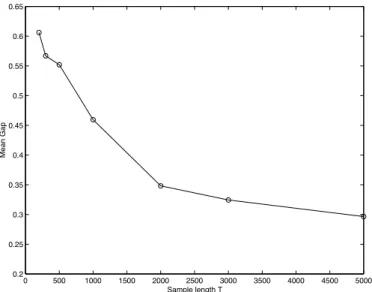
Source samples have been generated according to a discrete distribution with support {1, , −1, −}. Such sources are encountered in digital communications, when the (very common) QPSK modulation is used. They have as fourth order cumulants κ = 1 and ˜κ = −1. The data length T was varied from 200 to 5000 samples, and the mixing matrix was taken to be A = 0 0.81 + 0.39 0 0.35 + 0.35 0 0.5 − 0.86 0.86 1 .
A key issue is the choice of the performance measure. In the present case, it is not trivial to measure the error between the matrix identified by the algorithm, say ˆA, and the true mixing matrix A, since each column is computed up to a multiplicative complex number, and up to a permutation among the columns. In other words, one should measure the norm of ||A − ˆA · D||, for the best matrix D, formed of the product of a diagonal matrix and a permutation (such matrices are sometimes called generalized permutations). In order to do this, the basic tool is the computation of a distance Υ(u, v) between two vectors u and v, invariant up to a multiplicative complex number. For this purpose, one defines
Υ(u, v) = Min
z
||u − z v||2
||u|| · ||v||
It can be seen that if u†v= ||u|| · ||v|| · cos θ eψ, then the minimal distance Υ(u, v) is reached for || u ||u||−
v ||v||e−ψ||
and takes the value 2(1 − cos θ). The gap between two matrices is then computed as the minimum distance over the 6 possible permutations: Gap(A, ˆA) = Min P r ! i=1
Υ(coli(A), coli( ˆAP ))
The range of variation of this gap is thus [0, 6] in the present problem where r = 3. Note that this is easy to compute because of the very small dimension. For larger dimensions, one can avoid the exhaustive search for the best permutation by assuming another gap measure, of more complicated (but compact) form.9
In figure 1 the average gap obtained over 15 independent experiments is plotted. The gap keeps small (compared to its maximal achievable value of 6), even for a data length as small as T = 200. This behavior holds excellent as long as the noise is negligible. If noise is present, the performance degrades rather fast, especially for short data length T and non Gaussian noise. On the other hand, cumulant arrays are asymptotically insensitive to Gaussian noise (for large T ), providing some robustness to the method.
0 500 1000 1500 2000 2500 3000 3500 4000 4500 5000 0.2 0.25 0.3 0.35 0.4 0.45 0.5 0.55 0.6 0.65 Mean Gap Sample length T
3.4. Extension to larger dimensions
For dimensions n > 2, Sylvester’s theorem cannot apply. Instead, one should resort to Lasker-Wakeford theorem,4
whose proof is not constructive. Consequently, efficient blind identification algorithms still remain to be devised. But there are a number of results that are already known, especially concerning the rank (the width according to Reznick25). More precisely, for 2 ≤ n ≤ 8, it has been shown that the generic value of r is given by the following
table:4
r n 2 3 4 5 6 7 8 3 2 4 5 8 10 12 15 d 4 3 6 10 15 22 30 42
The number of free parameters that remain to be fixed in order to ensure uniqueness (in the sense that a finite set of equivalent solutions can be obtained) is given by the dimension of the manifold of solutions:4
n 2 3 4 5 6 7 8 3 0 2 0 5 4 0 0 d 4 1 3 5 5 6 0 6
One can check out, for instance, that for n = 2, we have indeed 1 free parameter to fix when decomposing 4-way arrays, whereas there are a finite number of solutions in the case of 3-way arrays. This has already been pointed out in section 3.2.1: a second 4-way cumulant array had been necessary in order to fix the parameter. It is interesting to notice that the latter property often holds true for 3-way arrays; on the contrary for 4-way arrays, it occurs only for n = 7 in the above table. Before to close this section, it is worth insisting that there is no simple rule or formula that would yield the values of these tables: it is the result of several theorems of various origins.4
4. NON LINEAR INVERSION OF THE LINEAR CHANNEL
In the previous section, the problem of blind identification of the mixture A has been addressed, but the recovery of the sources themselves was left open. In this section, it is assumed that the mixing matrix A is given, and the goal is to estimate the input (source) vector, x, from the observation vector, y. Because A has more columns than rows (under-determination), it cannot be linearly inverted.
4.1. Principle
In digital communications, the discrete-time processes always take values in a finite set. Therefore, their values can be completely characterized by a set of polynomial equations. Take the example of d−PSK modulated sources, which satisfy xd = 1. There are d solutions in the complex field, and hence a set of d allowed values. By adding to the n
observation equations (2) all the (n+dd+1) homogeneous monomials of degree d + 1, one gives oneself the opportunity to use the r additional equations xd
i = 1, 1 ≤ i ≤ r. The system can be solved thanks to these additional equations. In
order to illustrate the idea, we shall now consider the easiest case.
This system becomes especially simple when enough linear equations can be extracted. This is in particular the case if d = 2 and n = 2. In fact we have then r + 6 equations in r unknowns. The first 2 equations are given by (2). The next 4 equations are given by y3
1, y21y2, y1y22, y32. These equations involve products of the form x3i, x2ixj,
or xixjxk. By using the r remaining ones, namely x2j = 1, the latter products reduce simply to xi, xj, and xixjxk,
respectively. In other words, the system becomes almost linear, beside the (r
3) terms of the form xixjxk.
Now take our example of section 3, where r = 3. Then there is a single non linear term, x1x2x3. If this term is
considered as a plain unknown, independently of the 3 others, we end up with a linear system of 6 equations in 4 unknowns: # y z $ = # A 0 B $ · x1 x2 x3 x1x2x3 , where z = y3 1 y2 1y2 y1y22 y3 2 .
Since the 4 × 4 matrix B is a known function of A, it is given as soon as A is known. The above system can thus be solved for the 4 unknowns in the Least Squares (LS) sense. In the approach proposed here, the LS solution obtained for x1x2x3 is simply discarded.
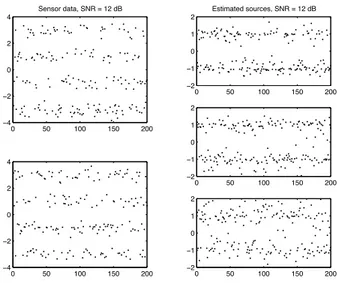
0 50 100 150 200 −4 −2 0 2 4 Sensor data, SNR = 12 dB 0 50 100 150 200 −4 −2 0 2 4 0 50 100 150 200 −2 −1 0 1 2 Estimated sources, SNR = 12 dB 0 50 100 150 200 −2 −1 0 1 2 0 50 100 150 200 −2 −1 0 1 2
Figure 2. Typical inversion results obtained with a SNR of 12dB.
4.2. Computer results
Data have been generated according to the following model:
y= A x + 1 ρw, where A = 0 2 0.1 −1 0.1 2 1 1
Parameter ρ allows to control the noise power. The signal to Noise Ratio (SNR) is defined here as 20 log10ρ. It is
thus a global value for the 3 sources, that implicitly depends on the matrix A, of course. Figure 2 shows a typical example, obtained for SNR=12dB. Note that the Signal to Interference Ratio (SIR) is of about 6dB for the first two sources, but of -6dB for the third one, measured on the space spanned by the exact directional vector. This yields an average SIR of about 3dB, coming in addition to the noise corruption.
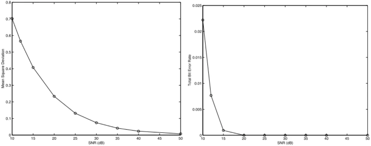
As the SNR varies from 10 to 50dB, two performance measures have been calculated. First, one has computed a mean standard deviation of the normalized source estimation error:
σerror= 8 3 ! i=1 variance 0 xi σ(xi) − xˆi σ( ˆxi) 191/2
where xi denotes the true source value of source i and ˆxi its estimate. Figure 3 (left) reports the performances
obtained. Second, the Bit Error Rate (BER) has been estimated over 10, 000 samples for each value of the SNR; the errors made for each of the 3 sources have been cumulated, so that the accuracy is 1/30, 000 ≈ 3.10−5. The BER
stays below 2 percent until 10dB (see figure 3, right).
5. CONCLUSION
One of the objectives of this paper was to demonstrate that it was possible to blindly identify a static system with more inputs than outputs, and to estimate its inputs from the outputs. The principles were illustrated in the case of n = 2 outputs and r = 3 inputs. The extension to larger numbers of inputs and outputs turns out to be much more complicated, and is still being studied. With this goal, other tracks can also be followed, as briefly explained in section 2.3. One of them, in the case of even orders (e.g. d = 4), is to consider the d−way array as an operator mapping the space of d/2−way arrays onto itself; another one is to attempt to compute the stationary values of Ωm.
Despite their potential usefulness, numerical algorithms have been to date only little studied.
ACKNOWLEDGMENTS
This work has been supported in part by the CNRS telecommunications program No.TL-97104, and in part by Eurecom’s industrial partners: Ascom, Cegetel, Hitachi, IBM France, Motorola, Swisscom, and Thomson CSF.
10 15 20 25 30 35 40 45 50 0 0.1 0.2 0.3 0.4 0.5 0.6 0.7 0.8 SNR (dB)
Mean Square Deviation
10 15 20 25 30 35 40 45 50 0 0.005 0.01 0.015 0.02 0.025 SNR (dB)
Total Bit Error Rate
Figure 3. Mean Standard Deviation (left) and Total Bit Error Rate (right) for the 3 estimates.
REFERENCES
1. J. B. KRUSKAL, “Three-way arrays: Rank and uniqueness of trilinear decompositions,” Linear Algebra and Applications 18, pp. 95–138, 1977.
2. J. D. CAROLL, S. PRUZANSKY, and J. B. KRUSKAL, “Candelinc: A general approach to multidimensional analysis of many-way arrays with linear constraints on parameters,” Psychometrika 45, pp. 3–24, Mar. 1980. 3. K. V. MARDIA, J. T. KENT, and J. M. BIBBY, Multivariate Analysis, Academic Press, 1979.
4. P. COMON and B. MOURRAIN, “Decomposition of quantics in sums of powers of linear forms,” Signal Pro-cessing, Elsevier 53, pp. 93–107, Sept. 1996. special issue on High-Order Statistics.
5. B. W. SILVERMAN, Density Estimation for Statistics and Data Analysis, Chapman and Hall, 1986.
6. P. COMON, “Supervised classification, a probabilistic approach,” in ESANN-European Symposium on Artificial Neural Networks, Verleysen, ed., pp. 111–128, D facto Publ., (Brussels), Apr 19-21 1995. invited paper. 7. E. CHAUMETTE, P. COMON, and D. MULLER, “An ICA-based technique for radiating sources estimation;
application to airport surveillance,” IEE Proceedings - Part F 140, pp. 395–401, Dec. 1993. Special issue on Applications of High-Order Statistics.
8. E. DeCARVALHO and D. T. M. SLOCK, “Cramer-Rao bounds for semi-blind, blind and training sequence based channel estimation,” in Proc. SPAWC 97 Conf., pp. 129–132, (Paris, France), Apr. 1997.
9. P. COMON, “Independent Component Analysis, a new concept ?,” Signal Processing, Elsevier 36, pp. 287–314, Apr. 1994. Special issue on Higher-Order Statistics.
10. J. F. CARDOSO, “High-order contrasts for independent component analysis,” Neural Computation , 1998. To appear.
11. P. McCULLAGH, Tensor Methods in Statistics, Monographs on Statistics and Applied Probability, Chapman and Hall, 1987.
12. L. TONG, “Identification of multichannel MA parameters using higher-order statistics,” Signal Processing, Elsevier 53, pp. 195–209, Sept. 1996. special issue on High-Order Statistics.
13. V. S. GRIGORASCU and P. A. REGALIA, “Tensor displacement structures and polyspectral matching,” in Fast Reliable Algorithms for Matrices with Structure, T. Kailath and A. H. Sayed, eds., ch. 9, SIAM Publ., Philadelphia, PA, 1998.
14. A. SWAMI, G. GIANNAKIS, and S. SHAMSUNDER, “Multichannel ARMA processes,” IEEE Trans. on Signal Processing 42, pp. 898–913, Apr. 1994.
15. L. DeLATHAUWER, Signal Processing based on Multilinear Algebra. Doctorate, Katholieke Universiteit Leuven, Sept. 1997.
16. X. R. CAO and R. W. LIU, “General approach to blind source separation,” IEEE Trans. Sig. Proc. 44, pp. 562– 570, Mar. 1996.
17. J. D. CAROLL and J. J. CHANG, “Analysis of individual differences in multidimensional scaling via n-way generalization of eckart-young decomposition,” Psychometrika 35, pp. 283–319, Sept. 1970.
18. G. M. BERGMAN, “Ranks of tensors and change of base field,” Journal of Algebra 11, pp. 613–621, 1969. 19. S. LEURGANS, R. T. ROSS, and R. B. ABEL, “A decomposition for three-way arrays,” SIAM Jour. Matrix
Anal. Appl. 14, pp. 1064–1083, Oct. 1993.
20. L. DeLATHAUWER, B. DeMOOR, and J. VANDEWALLE, A Singular Value Decomposition for Higher-Order Tensors. Second ATHOS workshop, Sophia-Antipolis, France, Sept 20-21 1993.
21. K. V. PARSHALL, “The one-hundred anniversary of the death of invariant theory,” The Mathematical Intelli-gencer 12(4), pp. 10–16, 1990.
22. J. A. DIEUDONN´E and J. B. CARREL, “Invariant theory, old and new,” in Computing Methods in Optimization Problems-2, pp. 1–80, Academic Press, (San Remo, Italy, Sept 1968), 1970.
23. E. K. WAKEFORD, “Apolarity and canonical forms,” in Proceedings of the London Mathematical Society, pp. 403–410, 1918.
24. R. EHRENBORG and G. C. ROTA, “Apolarity and canonical forms for homogeneous polynomials.” European Journal of Combinatorics, 1993.
25. B. REZNICK, “Sums of even powers of real linear forms,” Memoirs of the AMS 96, Mar. 1992. 26. B. REZNICK, “Sums of powers of complex linear forms.” Preprint, private correspondence, Aug. 1992. 27. L. DeLATHAUWER and B. DeMOOR, “From matrix to tensor: Multilinear algebra and signal processing,” in
Mathematics in Sig. Proc., IMA Conf. Series, Oxford Univ Press, (Warwick), Dec 17-19 1996.
28. J. F. CARDOSO and A. SOULOUMIAC, “Blind beamforming for nonGaussian signals,” IEE Proceedings -Part F 140, pp. 362–370, Dec. 1993. Special issue on Applications of High-Order Statistics.
29. J. F. CARDOSO, “Fourth-order cumulant structure forcing, Application to blind array processing,” in Proc. IEEE SP Workshop on SSAP, pp. 136–139, (Victoria), Oct. 1992.
30. P. COMON and J. F. CARDOSO, “Eigenvalue decomposition of a cumulant tensor with applications,” in SPIE Conf. Adv. Sig. Proc. Alg., vol. 1348, Arch. and Implem., pp. 361–372, (San Diego, CA), July 10-12 1990. 31. L. DeLATHAUWER, P. COMON, et al., “Higher-order power method, application in Independent Component
Analysis,” in NOLTA Conference, vol. 1, pp. 91–96, (Las Vegas), 10–14 Dec 1995.
32. P. COMON, “Cumulant tensors”. IEEE SP Workshop on HOS, Banff, Canada, July 21-23 1997. Keynote address, www.i3s.unice.fr/~comon/plenaryBanff97.html.