HAL Id: hal-02307255
https://hal.archives-ouvertes.fr/hal-02307255
Submitted on 7 Oct 2019
HAL is a multi-disciplinary open access
archive for the deposit and dissemination of
sci-entific research documents, whether they are
pub-lished or not. The documents may come from
teaching and research institutions in France or
abroad, or from public or private research centers.
L’archive ouverte pluridisciplinaire HAL, est
destinée au dépôt et à la diffusion de documents
scientifiques de niveau recherche, publiés ou non,
émanant des établissements d’enseignement et de
recherche français ou étrangers, des laboratoires
publics ou privés.
Vadose Zone Modeling in a Small Forested Catchment:
Impact of Water Pressure Head Sampling Frequency on
1D-Model Calibration
Benjamin Belfort, Ivan Toloni, Philippe Ackerer, Solenn Cotel, Daniel Viville,
François Lehmann
To cite this version:
Benjamin Belfort, Ivan Toloni, Philippe Ackerer, Solenn Cotel, Daniel Viville, et al.. Vadose Zone
Modeling in a Small Forested Catchment: Impact of Water Pressure Head Sampling Frequency on
1D-Model Calibration. Geosciences, Geological Survey of Iran, 2018, 8 (2), pp.72.
�10.3390/geo-sciences8020072�. �hal-02307255�
Geosciences 2018, 8, x; doi: FOR PEER REVIEW www.mdpi.com/journal/geosciences
Article
Vadose Zone Modeling in a Small Forested
Catchment: Impact of Water Pressure Head Sampling
Frequency on 1D-Model Calibration
Benjamin Belfort *, Ivan Toloni, Philippe Ackerer, Solenn Cotel, Daniel Viville and François Lehmann
Université de Strasbourg, CNRS, ENGEES, LHYGES UMR 7517, F-67000 Strasbourg, France; itoloni@unistra.fr (I.T.); ackerer@unistra.fr (P.A.); cotel@unistra.fr (S.C.); dviville@unistra.fr (D.V.); lehmann@unistra.fr (F.L.)
* Correspondence: belfort@unistra.fr; Tel.: +33-368-850-386
Received: 19 January 2018; Accepted: 13 February 2018; Published: date
Abstract: The characterization of vadose zone processes is a primary goal for understanding,
predicting, and managing water resources. In this study, the issue of soil water monitoring on a vertical profile in the small forested Strengbach catchment (France) is investigated using numerical modeling with the long-term sequences 1D-Richards’ equation and parameter estimation through an inverse technique. Three matric potential sensors produce the observation data, and the meteorological data is monitored using an automatic weather station. The scientific questions address the selection of the calibration sequence, the initial starting point for inverse optimization and monitoring frequency used in the inverse procedure. As expected, our results show that the highly variable data period used for the calibration provides better estimations when simulating the long-term sequence. For the starting point of the initial parameters, handmade iterative initial parameters estimation leads to better results than a laboratory analysis or set of ROSETTA parameters. Concerning the frequency of monitoring, weekly and daily datasets provide efficient results compared to hourly data. As reported in other articles, the accuracy of the boundary conditions is important for estimating soil hydraulic parameters and accessing water stored in the layered profile.
Keywords: forested catchment; hydrology; sensor monitoring; matric potential; parameter
estimation; numerical modeling; one-dimensional simulations
1. Introduction
The thin layer of the Earth’s surface from the top of the vegetation canopy to the bottom of the weathering zone has been called the ‚Critical Zone‛ (CZ). The CZ is also subject to increasing anthropogenic perturbations due to human activities [1]. Hence, the monitoring, understanding, and modeling of the CZ are compelling research activities in Earth and environmental sciences during the 21st century [2].
Among the various topics investigated by the CZ science community, the soil-plant-atmosphere continuum (SPAC) is of interest, because it links aboveground and belowground systems. The interactions between these two systems address the water flow in soil and concurrent plant root water uptake [3], the influence of precipitation partitioning [4,5], the interaction between vegetation distribution, climate, and soil moisture spatial patterns [6], and the interaction between surface and subsurface processes at the catchment scale [7,8]. SPAC leads to the examination of the vadose zone (VZ), also called the unsaturated zone, which is the portion of the subsurface located above the groundwater table. Processes occurring in the VZ can strongly affect the quality of water and the
rate of aquifer recharge, which are critical issues for the use and management of groundwater. In the context of climate change [1], one of the key variables for understanding and modeling hydrological processes, as well as for developing predictive numerical tools to manage human activities (agricultural, industrial, domestic, etc.), is soil moisture [9].
Different methods may be used to estimate the soil moisture, which mainly include in situ methods [10], satellite-based data retrieval [11–13], and hydrological model based results [14]. The various available methods are generally combined to take advantage of their respective assets [15–17], as temporal-spatial scale issues and human-economic means dedicated to monitoring are important limiting factors. In the context of hydrology data assimilation, soil water is a key variable to be integrated into a model to predict the state and evolution of a system [16]. Hence, reliable in situ measurements are of considerable interest and have received increasing attention in recent studies. The issues of measurements and numerical models have been largely handled in the literature, which focuses on either technical sensor specifications, scale definitions and spatial averaging aspects, processes and parameters characterization, or data aggregation methods, and so on [17–20]. Nonetheless, as noticed by Vereecken et al. [16], improved measurement and modelling methods must be combined to advance the science of the vadose zone and catchment hydrology. In the present article, monitoring strategies established in the Strengbach catchment for local measurements of water matric potential are addressed.
Our study is mainly focused on the integration of monitored data to access soil parameters, which can strongly affect the reliability of numerical simulations. To model water flow in the VZ, hydraulic parameters characterizing the soil, i.e., water retention curves and unsaturated hydraulic conductivity functions, must be defined [21]. To satisfy this characterization, direct measurement methods generally require soil samples followed by laboratory analysis. In situ measurements that include tension and pressure infiltrometers may be completed with the classic, undisturbed soil core methods in a laboratory [22]. The generalization of this approach to field scale applications is difficult, expensive and adaptation to modeling issues for flow and transport processes might require further discussion because of perturbation or the representativeness of small soil cores and scaling effects [23]. Hence, the development of indirect methods to derive soil hydraulic properties at the application scale of the model has gained popularity. On the one hand, parameter estimation using an inverse modeling approach based on flux data is often combined with measurements of matric potential, and this has become a common practice at the column scale [16,24]. On the other hand, only a limited number of studies use field scale measurements to inversely estimate soil hydraulic properties [16]. In their review paper, Vereecken et al. [16] argued that the selection of measurements is a critical point to provide physically reasonable estimates of hydraulic parameters. As a limiting factor, they also claimed that successful inversions require constraining parameters with additional information regarding measured matric potential, soil structural information, homogeneous soil assumptions, measured values of hydraulic properties, well-defined flow conditions with gravity-dominated flow, and known bottom boundary conditions. Therefore, inverse parameter estimation from field scale soil measurements under naturally occurring boundary conditions is a challenging issue, which has been moderately investigated.
Nonetheless, a few (non-exhaustive list) examples are discussed here in the abovementioned context. The time series of water content and/or matric potential monitored at experimental sites has been reported by Jacques et al. [25], Ritter et al. [26,27], Ireson et al. [28], Wollschläger et al. [29], Scharnagl et al. [30], Andreasen et al. [31], Mathias et al. [32], Thoma et al. [33], Seki et al. [34], Singh et al. [35], Broca et al. [36], and Hawke and McConchie [37]. We retain from these studies the following information: (i) laboratory soil characterization (textural, structural, water retention curves) provides useful additional information; (ii) fluxes at the soil surface (rainfall and evapotranspiration) and, to some extent, at the bottom of the profile are of great importance; (iii) the application of Richards’ equation (RE) to model water flow in the VZ under natural conditions may lead to efficient results; (iv) a combination of input data may be sufficient for suitable parameter estimation; and (v) unsaturated hydraulic properties obtained through inverse parameter modeling are affected by a strong non-uniqueness of the inverse problem, which makes it difficult to find an
‚ideal‛ set of parameter values in natural field conditions. These points have been considered in the present article: RE has been used, different additional information about soil and hydraulic behavior has been integrated to constrain parameter estimation and a specific focus has been placed on boundary fluxes estimation.
Another issue not yet addressed in this introduction is the frequency of measurements and their possible aggregation. Depending on the devices-site extension or treated subjects, measurement frequencies used in field monitoring are very disparate: 3 min [33], 5 min [37], 10 min [29,34], 15 min [37], 30 min [28,31], 1–2 or 3 h [25,29,30,33,35], 1 day [28,32], or 1 week [28]. Data are sometimes averaged over time or space to satisfy the constraints of numerical tools [35], minimize temporal correlation [31], investigate variability [36], and synchronize the frequency of monitoring devices or facilitate global interpretation [30,32]. These various articles highlight the difficulty in addressing field measurements and establishing a generic monitoring scheme. This overview does not permit the establishment of a general rule to define the frequency of measurements, the spatial or temporal averaging strategy to be implemented for the handled subject, and the extension of the experimental site. In the present article, the issue of monitoring resolution and its connection to parameter estimation will be addressed.
The scientific challenges resulting from climate and global change have raised the issue of data monitoring in many observatories, which are concerned with long-term observations and research in multi-compartment and multi-scale domains. The present study will describe an inverse parameters estimation approach based on measurements achieved under natural conditions at the experimental site of the Strengbach forested catchment. Hence, matric potential on a vertical profile and rainfall intensity were monitored and used to estimate the hydraulic properties of a heterogeneous forest soil. The originality and difficulty of this work relies on natural field conditions that have been considered. The second original point addresses the impact of the measurement frequency on the estimated parameters. To the best of our knowledge, this issue has not been addressed in this context. Hence, our purpose is to define a methodology that will take the best parts of different measurements obtained at the site to optimize its description in a potentially predictive numerical modeling approach.
This study could also serve to generalize the monitoring strategy at other locations in the catchment and to progressively obtain a general characterization that could be helpful for numerical simulations of hydrological processes in a 3D domain. The introduction section provides general motivations to study hydrological processes that occur in the VZ. A brief overview of field studies focusing on soil water is proposed. The interest in monitoring soil water variables and the difficulties encountered in this domain are underlined throughout different previous articles. The second section of this paper is dedicated to the description of the site, materials used for in situ measurements, available soil properties based on sampling and laboratory analysis, and the numerical method used for parameter estimation. In Section 3, the dataset is described and parameter estimation based on inverse modeling is discussed.
2. Materials and Methods
2.1. Site Description and Monitoring Devices
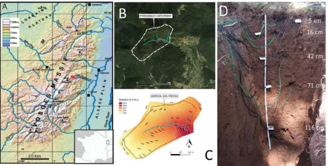
The present study was conducted in the forested Strengbach catchment, which is in the Vosges Mountains (northeastern France) (Figure 1A). This small watershed of 0.8 km2 has become a
completely equipped environmental observatory with permanent sampling and measuring stations that have been in operation since 1986. This watershed is the study site of the Observatoire Hydro-Géochimique de l’Environnement (OHGE, http://ohge.unistra.fr) and belongs to the French and European networks of Critical Zone observatories. With altitudes ranging from 883 to 1146 m (Figure 1B,C), the current climate is mountainous-oceanic with a mean annual rainfall of 1400 mm and an average temperature of approximately 6 °C [38]. The site is well suited for multidisciplinary studies in hydrological, geochemical and forest research [39–42].
Figure 1. (A) Regional map of the Vosges Massif and location of the Strengbach catchment. (B)
Contour map of the Strengbach watershed. (C) Topographic map of the Strengbach watershed and location of the studied weathering profile (map from OHGE). (D) Vertical profile in the experimental spruce parcel (blue star in Figure 1C) where sensors have been installed.
The monitoring devices have been installed in a 100-year-old spruce experimental stand located in the northern upper portion of the Strengbach catchment (Figure 1C,D, ALT: 1079 m; COORD: 48°12.963’ N and 7°11.928’ E). This parcel is representative of a large part of the domain, which is 90% covered by forest, which consists of 80% spruce and 20% beech. For hydrological instrumentation, a pit of approximately 1.30 m in depth and 0.70 m in width has been implemented between the trees during September 2010. Several probes, 5 Watermark sensors including a Campbell 257 for matric potential, and 4 Campbell 107 probes for temperature (the deeper location was not equipped) were horizontally inserted in the wall of the pit at five different depths (5, 16, 42, 71, and 116 cm). Automatic data acquisition is obtained by the 9 sensors using a Campbell Scientific®
CR1000 datalogger with a measurement frequency of 10 min, according to other devices monitored in the catchment. All the connecting wires were protected with a 40-mm flexible plastic tube to avoid instrumentation damage. After the in situ installation of these devices, the hole was refilled trying to maintain the natural order of the different layers of soil as close as possible to reduce soil disturbance.
The Watermark sensor is a solid-state, electrical resistance sensing device with a granular matrix that estimates soil water potential between 0 and −2 bars. The matric potential (MP) values are calculated from resistance values (kOhm) using the following equations [43–45]:
21 21 7.407 3.704 1 0.018 s MP R R R dT (1)where MP is the matric potential (kPa), R21 is the resistance at 21 °C, Rs is the measured resistance, and dT T S21 Ts are the soil temperature. After preliminary tests conducted in the laboratory, the previous linear calibration relationship proposed by the manufacturer (Equation (1)) appeared to be well suited compared to the proposed nonlinear calibration relationship.
The time series of precipitation, air temperature, relative humidity, wind speed, and solar radiation were obtained from a meteorological station located in a nearby clearing. These climatic variables monitored every 10 min were used to calculate potential evapotranspiration, which has been previously underlined as an important parameter controlling the applied boundary flux. The
data validation process of the pressure sensors led to discarded records for depths of 5 cm and 16 cm due to aberrant measurements. In this upper part of the profile and during different periods between 2011 and 2016, the pressure measurements were in contradiction with the monitored incoming flux; for example, these sensors show decreasing pressure heads while the soil was receiving rainwater. Despite the great focus given to preparation and field installation, this problem can be explained by a bad soil to sensor contact when positioning the probes and/or by disturbances related to the climatic conditions (such as ground freezing).
2.2. Vertical Profile and Soil Properties
During the probe installation operations, many soil samples were collected and subjected to laboratory analysis. Each sample was characterized in the following manner:
The hydraulic retention curve was determined (soil moisture as a function of pressure head);
The saturated hydraulic conductivity (Ksat) was estimated through 9 constant head permeability
tests (Table 1). The measures concerning the layer between −15 cm and −20 cm were discarded due to their abnormally large values and large standard deviation. For the same reason the first measure of each sample was discarded;
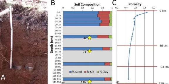
The composition of the soil was determined through a laser diffraction particle sizing technique (Figure 2). The soil was mainly composed of sand (70–80%). A strong gradient of porosity can be observed over the first 15 cm, which is probably related to the richness of organic matter in this soil layer (Figure 2C).
Figure 2. (A) Undisturbed soil cylinder samplers. (B) Soil composition profile; yellow stars
correspond to sampling points and (C) porosity profile obtained through laboratory analysis of the field samples. These values are used for the ROSETTA pedotransfer function. The red lines in (C) represent the interfaces between the three layers of the adopted soil model.
Samples were obtained from nine depths (Figure 2A); nonetheless, due to the restriction in operating devices and the complexity of parameter estimation under natural conditions, the domain discretization was simplified. Previous investigations in the catchment and local sampling at the bottom of the pit with a soil auger led to the consideration of a vertical profile of 150 cm depth. In addition, the soil composition (Figure 2B) and porosity profile (Figure 2C) may suggest simplifying the domain by considering two zones of approximately 50 cm on each side of the transition zone. Since two sensors have been installed at 71 and 116 cm, and to bring more flexibility to our inverse parameter estimation procedure, we have increased the number of degrees of freedom by dividing this deeper area into two zones. Finally, the horizons are placed halfway between the three lowest sensors (depths: 42 cm, 71 cm, and 116 cm). The first layer is from the soil surface to 56 cm, the
second layer is from 56 cm to 93 cm, and the third layer is from 93 cm to 150 cm. The data from the nine depths were fitted together to obtain the parameters of the three layers.
2.3. Numerical Models
2.3.1. Potential and Actual Evapotranspiration
The estimation of the potential evapotranspiration (PET) is important for modeling the water flux at the soil surface [46,47]. Following Biron [48], the computation of PET for our forested catchment is based on the Penman model and is achieved according to the procedure given by Brochet and Gerbier [49] (PETBG in Equation (2)). Previous studies have shown that this approach
considers the specificities of the experimental site, especially for the computation of the net radiation in the radiative term (first component of the r.h.s. term in Equation (2)) and the expression of the advective term (second component of the r.h.s. term in Equation (2)). Hence, to remain consistent with previous studies of the Strengbach catchment, the following equation was adopted:
n
BG 10 eR
1
PET
0.26
1 0.4 u
59
(2)PETBG is given in mm·d−1,
is the derivative of saturated vapor pressure versus temperature(mbar·K−1) expressed as the air temperature Ta (°C) (see Equation (3)), Rn is the net radiation at the
canopy surface (cal·cm−2·d−1),
e
is the saturation vapor pressure deficit (mbar) expressed at the air temperature Ta (°C) and the relative humidity Hr (%) (see Equation (4)),
is the psychrometricconstant (0.66 mbar·K−1) and U10 is the adjusted wind speed at 10 m height (m·s−1).
a a 7.5 T 237.3 T 2 a 25039 10 237.3 T (3)
aa 7.5 T 237.3 T e 1 Hr 6.107 10 (4)Originally, the estimation of net radiation was based on global radiation measurements and a table of sunshine duration for potential corrections. Hence, the previous equations (Equations (2)–(4)) have allowed for the computation of daily PETBG; since the data are available at a 10-min time step,
net radiation is cumulated every hour and other variables were averaged to obtain hourly PETBG.
Notice that the cumulated values of hourly PETBG are in concordance with daily or weekly
estimations. Between January 2011 and December 2016, the amount of rainfall reached 1228 mm/year, and the amount of PETBG is 446 mm/year.
If PET represents the maximal evapotranspiration under well-watered conditions, the actual evapotranspiration (AET) considers the hydric stress and precipitation intercepted and evaporated
by conifer foliage during different seasons. Using BILJOU© software
(https://appgeodb.nancy.inra.fr/biljou/) [50], the AET was calculated as follows:
AET Tr In SEvap (5)
where Tr refers to transpiration by the canopy (mm·d−1), In is the interception (mm·d−1) and SEvap is
the soil and understored evaporation (mm·d−1).
Climatic variables such as PET and recorded precipitations are provided to BILJOU as input data, together with the site characterizing parameters, which concern canopy, plant interception, soil evaporation and changing of the seasons. The three contributions to AET in Equation (5) are partly driven by the maximum leaf area index (LAI), which is a dimensionless quantity that characterizes plant canopies and is defined as the projected leaf area per unit ground area (in this study LAI = 7). AET is calculated from BILJOU using a daily time step. Runoff has never been observed on the experimental parcel due to the vegetation cover. Therefore, considering that this type of surface– subsurface interaction in the model is not required, the application of BILJOU software is possible.
Between January 2011 and December 2016, 12.1% of the rainfall amount was intercepted from the canopy, 13.5% returned to the air by transpiration and 1.4% was evaporated from the soil. Approximating the infiltrated water flux as the difference between rainfall and AET, it follows that 73% (896.7 mm) of the precipitation (1228 mm) infiltrated the soil.
2.3.2. Vadose Zone Model
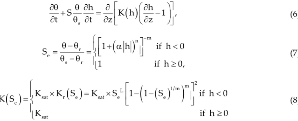
The adopted hydrological model is composed of the Richards’ Equation (6), which describes water movement in a variably saturated, porous medium. Furthermore, the standard Mualem-van Genuchten model (Equations (7) and (8)) describes the interdependencies between the pressure head (h), water content (θ), and relative conductivity (Kr) [51,52]:
s h h S K h 1 , t t z z (6)
n m r e s r 1 h if h 0 S 1 if h 0, (7)
2 m 1/ m L sat r e sat e e e sat K K S K S 1 1 S if h 0 K S K if h 0 (8)where S is the storage coefficient [L−1], Se is the effective saturation [-], θ is the volumetric water
content [L3·L−3], θs is the saturated water content [L3·L−3], θr is the residual water content [L3·L−3], h is
the pressure head [L], K is the hydraulic conductivity [L·T−1], z is the vertical distance positive
downward [L], t is the time [T], α is a parameter related to the mean pore size [L−1], n is a parameter
reflecting the uniformity of the pore size distribution [-], m is a parameter defined by (m 1 1 n) [-] [51], Ksat is the saturated hydraulic conductivity [L·T−1], and L is a parameter related to the tortuosity
chosen here equal to 0.5 [-] [52].
A set of 5 parameters (Ksat, θs,θr, n, α) is needed for each layer of the considered domain. The
hydraulic retention curves described in Section 2.2 were fitted to estimate the 5 parameters for a 3-layer profile (Table 1). In each layer, data coming from the sampling analyses of the 9 layers were aggregated to correspond to the 3 layers of the discretized domain. A second estimation of the hydrodynamic parameters was obtained from soil granulometry and bulk density through the ROSETTA pedotransfer function [53].
Table 1. Estimation of hydrodynamic parameters obtained through fitting the hydraulic retention
curves and ROSETTA pedotransfer function. The Ksat value of the first parameter set was obtained
using the constant head permeability test.
Layer
Retention Curve Fit ROSETTA Ksat (cm/day) θr (-) θs (-) α (1/cm) n (-) Ksat (cm/day) θr (-) θs (-) α (1/cm) n (-) 1 805 0.2 0.5 0.08 1.60 202 0.04 0.48 0.034 1.46 2 843 0.2 0.5 0.10 1.40 213 0.04 0.41 0.041 1.92 3 1616 0.0 0.5 0.40 1.15 262 0.04 0.42 0.041 1.96 2.4. Numerical Simulations
Simulations for the years 2012 to 2016 were run using ‚WaMoS-IPE-1D‛ (water movement in soil–inverse parameters estimation–1-dimensional). Numerical methods used in this Fortran computational code to solve the RE (Equation (6)) consist of the following: (i) a finite element method for spatial discretization; (ii) backward Euler scheme (full implicit) for temporal approximation; (iii) variable switching method with modified Picard or Newton methods for the
linearization strategy [54]; (iv) heuristic time stepping scheme based on the number of iterations for progression over time [55]; (v) a switching, flux-controlled procedure for the management of the top boundary condition (to preserve physical results) [56]; and (vi) Levenberg-Marquardt iterative algorithm to solve the inverse problem. A complete description of the code can be found in Lehmann and Ackerer [57]. A uniform mesh with 1 cm node spacing has been used for the spatial discretization of the domain. An initial pressure head profile was adopted as follows. High suction was initially assigned to the soil surface to facilitate water infiltration (htop = pF 4). The initial
pressure head profile is then obtained through the interpolation of the values measured at −42 cm, −71 cm, and −116 cm. Each simulation was subjected to a sufficiently long warm-up period so that no impact of the initial pressure head profile on parameter estimation was observed. An imposed flux boundary condition (BC) was applied to the soil surface, which was combined with a free drainage bottom BC.
A preliminary work has been achieved to validate the flux BC, which results from a combination of rainfall intensity and AET. Despite the simulated period, consideration of the raw rainfall data collected at the nearby meteorological weather station led to a systematic overestimation of humidity in the upper part of the soil profile. On the other hand, the AET was not subject to such an impact, especially during the dry period. Among several tested combinations, the most efficient and acceptable solution to construct the BC consisted of retaining 80% of precipitation data and subtracting the total amount of AET. In other words, the precipitation data likely had to be adjusted because of its required input data spatial adaptation for the specific location of the vertical profile. Simultaneously, the BILJOU parametrization, which was used in previous unpublished studies dealing with water balance estimation, was considered reliable, and therefore, it has been retained to estimate AET. Simulations were run using hourly, daily, and weekly BC frequencies. The BILJOU software estimates daily AET, and the weekly AET was obtained by cumulating daily AET. We assumed that the AET followed the same distribution over the course of a day as the PET, and consequently, the hourly AET was obtained as follows:
h h day day PET AET AET PET (9)
2.5. Strategies Investigated for the Model Calibration
The model was calibrated minimizing an objective function, which is defined as the square difference between pressure head measured values (hi) and simulated values
ˆhi :
inv N 2 i i i 1 ˆ O h h
(10)where Ninv is the amount of data (3 times the number of hourly, daily or weekly observation times)
used for the inverse problem.
As previously stated, the iterative solution to the inverse problem was obtained by applying the Levenberg-Marquardt algorithm [58]. The effectiveness of the calibrations was evaluated through the objective functions value and information indicators such as the Akaike information criterion (AIC) and Bayesian information criterion (BIC) [59,60]. The AIC and BIC provide a measure of the relative quality of a model for a given set of data, which considers the number of data, number of model parameters, and the value of the objective function:
p inv inv
AIC=2N +N Log(O/N )
(11)p inv inv inv
BIC=N Log(N )+N Log(O/N )
(12)where Np is the amount of parameters, Ninv is the amount of data used in the inverse problem, and O
is the objective function value after minimization. The smaller the criterion value, the better the calibration.
Our parameter estimation strategy involved the comparison of the effects of data monitoring frequencies, calibration periods, and initial parameter descriptions for the calibrated parameters. Hence, the model was calibrated with data from two periods. The first period, which was from June to September 2012, represents an average annual sequence. The second period, which was from April to December 2015, constitutes an unusual sequence that includes a dry period with low-pressure values in the profile. The inverse simulations related to the first and second periods were preceded by a warm-up period of 5 months and 3 months, respectively, to reduce the potential impacts of errors in initial conditions.
The model was calibrated with pressure head data presenting hourly, daily, or weekly frequencies (Figure 3). Since the collected observation data have a 10-min frequency, the required frequency was obtained through virtual sampling, i.e., by choosing one data point every hour, every day, or every week, without averaging the physical variables. The temporal discretization of BC leads to equivalent flux conditions, despite the time step size, i.e., the weekly or daily BC correspond to the accumulation of the hourly BC. As a starting point, several sets of parameters were tested for the optimization. Neither the parameters obtained through laboratory measurements nor the parameters obtained through the ROSETTA pedotransfer function led to a good match between measured and computed pressures. The best starting set of parameters was found empirically and is closer to the ROSETTA parameters than to the laboratory parameters (Table 2). The calibration process involved parameters Ksat, n, and α. Parameters θs andθr have empirically determined
assigned values due to the difficulties in their optimization and to decrease the problems’ degrees of freedom.
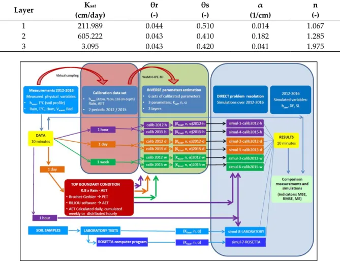
Table 2. Initial values of the hydraulic parameter estimation procedure using inverse modeling.
Layer Ksat (cm/day) θr (-) θs (-) α (1/cm) n (-) 1 211.989 0.044 0.510 0.014 1.067 2 605.222 0.043 0.410 0.182 1.285 3 3.095 0.043 0.420 0.041 1.975
Figure 3. Conceptual scheme of the modeling approach. The data frequency changes at different
steps during the process. The initial measured data and final simulated data have a 10-min time step. However, throughout the process, data with hourly, daily, and weekly time steps are used. The hmes
(hsim) is measured (simulated) pressure head, T °C is temperature, rain is rainfall, AET is the
calculated actual evapotranspiration, Ksat is the saturated hydraulic conductivity, α and n are parameters for the Mualem-van Genuchten model, DF is the drained flux at −150 cm, SL is the saturation level, MBE is the mean bias error, RMSE is the root mean square error, and ME refers to the modeling efficiency.
A global description of the modeling approach is summarized in Figure 3. This figure depicts the various steps, which include preparation of the data according to the selected frequency, constitution of the top boundary condition, estimation of parameters during the two calibration periods, direct simulations over the complete period, and analysis of results using statistical indicators.
3. Results
3.1. Parameters
The parameters optimized using hourly, daily, and weekly pressure head data for the periods from June to September 2012 and from April to December 2015 are shown in Table 3. The standard error (SE) for each estimated parameter was computed as follows:
1 T inv p O J J N SE N (13)
where J is the Jacobian matrix whose coefficients are the derivatives of predicted pressure head with respect to model parameters [57,61].
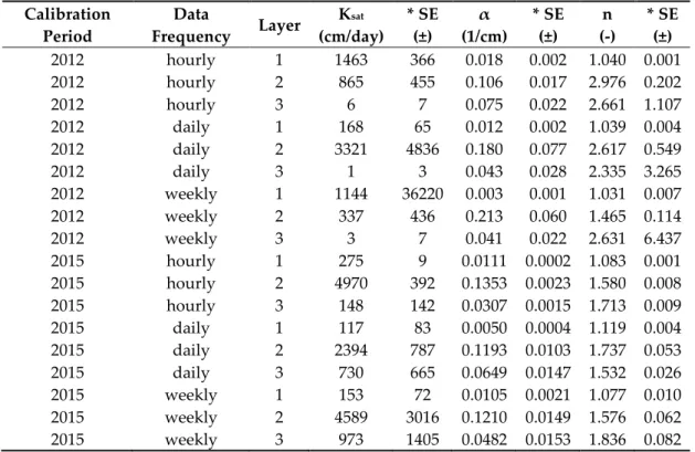
Table 3. Optimized parameters using hourly, daily, and weekly pressure head data. Data are
selected from two periods: from June to September 2012 and from April to December 2015. The adopted values of θs andθr are shown in Table 1.
Calibration Period Data Frequency Layer Ksat (cm/day) * SE (±) α (1/cm) * SE (±) n (-) * SE (±) 2012 hourly 1 1463 366 0.018 0.002 1.040 0.001 2012 hourly 2 865 455 0.106 0.017 2.976 0.202 2012 hourly 3 6 7 0.075 0.022 2.661 1.107 2012 daily 1 168 65 0.012 0.002 1.039 0.004 2012 daily 2 3321 4836 0.180 0.077 2.617 0.549 2012 daily 3 1 3 0.043 0.028 2.335 3.265 2012 weekly 1 1144 36220 0.003 0.001 1.031 0.007 2012 weekly 2 337 436 0.213 0.060 1.465 0.114 2012 weekly 3 3 7 0.041 0.022 2.631 6.437 2015 hourly 1 275 9 0.0111 0.0002 1.083 0.001 2015 hourly 2 4970 392 0.1353 0.0023 1.580 0.008 2015 hourly 3 148 142 0.0307 0.0015 1.713 0.009 2015 daily 1 117 83 0.0050 0.0004 1.119 0.004 2015 daily 2 2394 787 0.1193 0.0103 1.737 0.053 2015 daily 3 730 665 0.0649 0.0147 1.532 0.026 2015 weekly 1 153 72 0.0105 0.0021 1.077 0.010 2015 weekly 2 4589 3016 0.1210 0.0149 1.576 0.062 2015 weekly 3 973 1405 0.0482 0.0153 1.836 0.082 * Standard error.
The optimizations using the 2012 data result in Ksat values with very large SE, which means that
this parameter has little influence on pressure head. Generally, the saturated hydraulic conductivity is known to be a very sensitive parameter [62,63]. Here, the large SE could be related to the lack of
dynamics in the pressure head values at depths of 71 cm and 116 cm, as well as to the small pressure variations during 2012. The 2015 optimized values also have quite a large SE value, but a value smaller than the 2012 SE. The optimized Ksat values are very large compared to the values estimated
by the ROSETTA pedotransfer function and constant head permeability test (Table 1). Moreover, if previously estimated values are larger for the third layer, optimized values are larger for the first or second layer. This may be due to a higher organic matter content. The ‚n‛ optimized values for the first layers are typical of clay-rich soils.
3.2. Simulation Quality Estimation
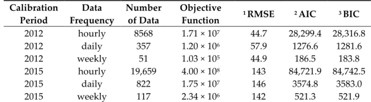
According to the AIC and BIC criteria (Table 4), the best calibrations are those performed using weekly data, followed by daily and hourly data. Since the best statistical criteria values are obtained from the calibrations using the smaller dataset, this selection based on AIC and BIC criteria could be influenced by the number of data involved in the inverse optimizations. Normally, AIC and BIC consider the amount of data, but the applied weight was not sufficient. Similarly, the calibrations using the 2012 data obtain better results than those using the 2015 data, which are performed over a longer period. The root mean square error (RMSE), which is defined in Equation (14), has also been computed to compare the different calibrations. The RMSE values reported in Table 4 corroborate previous conclusions that result from the AIC and BIC criteria.
inv N i i i dir h h RMSE N
2 1 ˆ (14)where Ninv refers to the number of pressure head measurements used in the inverse parameters
estimation (Ninv = number of data in Table 4) and Ndir refers to the number of pressure head
measurements used for the comparison of direct problem solutions.
Table 4. Parameters characterizing the effectiveness of calibrations.
Calibration Period Data Frequency Number of Data Objective Function
1 RMSE 2 AIC 3 BIC
2012 hourly 8568 1.71 × 10⁷ 44.7 28,299.4 28,316.8 2012 daily 357 1.20 × 10⁶ 57.9 1276.6 1281.6 2012 weekly 51 1.03 × 10⁵ 44.9 186.5 183.8 2015 hourly 19,659 4.00 × 10⁸ 143 84,721.9 84,742.5 2015 daily 822 1.75 × 10⁷ 146 3574.8 3583.0 2015 weekly 117 2.34 × 10⁶ 142 521.3 521.9
1 Root mean square error; 2 Akaike information criterion; 3 Bayesian information criterion.
To evaluate the effectiveness of the direct simulations, 3 indicators have been computed: the RMSE (Equation (14)), mean bias error (MBE Equation (15)), and model efficiency (ME Equation (16)). These indicators were calculated from simulated pressure head values and observed values with a resolution of 10 min over the entire 2012–2016 period. These values are presented in Table 5 with the goal of identifying the impact of the different calibrations (Table 3) on the predictive simulations [54] [64].
dir N i i i 1 dir ˆh h MBE N
(15)
dir Lk k N 2 i i i 1 N 3 2 i L k 1 i 1 ˆh h ME 1 h h
(16)where Ndir refers to the number of pressure head measurements used for the comparison of direct
problem solutions (Ndir = 3 × 227,371 = 628,113), k
L
h refers to the mean observed pressure head in layer Lk (k = 1, 2 or 3), and NLk refers to the number of values originating from layer Lk. Notice that
the RMSE in Table 5 was computed using Ndir instead of Ninv. The desired value for ME is one,
whereas the desired values for MBE and MRSE are zero. The modeling efficiency, ME, is a global model performance measure that provides the ratio of deviations regarding the measured values. It compares the square difference between the modelled and measured heads (numerator) with the square difference between the average measured values and the measured values (denominator). The RMSE statistical measure is an average error obtained through a term by term comparison of the square difference between the simulated and observed values. Hence, errors are cumulated using RMSE, whereas the MBE value is a relative measure that distinguishes between under and overestimation. MBE is positive (resp. negative) when the computed values are greater (resp. smaller) on average than the measurements.
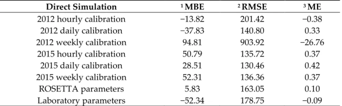
Table 5. Statistical measures for direct simulations over the period from 2012 to 2016 using eight
different sets of parameters (see Figure 3). All the sets of parameters were obtained through calibration except for the ROSETTA parameters set and laboratory parameters set. The statistical measures are related to the entire profile, and those referring to each layer are provided as supplementary material.
Direct Simulation 1 MBE 2 RMSE 3 ME
2012 hourly calibration −13.82 201.42 −0.38 2012 daily calibration −37.83 140.80 0.33 2012 weekly calibration 94.81 903.92 −26.76 2015 hourly calibration 50.79 135.72 0.37 2015 daily calibration 28.51 130.46 0.42 2015 weekly calibration 52.31 136.36 0.37 ROSETTA parameters 5.83 163.05 0.10 Laboratory parameters −52.34 178.75 −0.09
1 Mean bias error 2 root mean square error 3 model efficiency.
According to the RMSE and ME, the best model performances over the period of 2012–2016 are those using the 2015 calibrations. This could be related to the fact that in 2015, pressure head measures reached high negative values that significantly impacted the RMSE. The calibration using daily sampled data resulted in simulations with a slightly smaller RMSE and a larger ME than other sampling frequencies. The model predictions obtained using the set of parameters from the ROSETTA pedotransfer function and the retention curve fit (laboratory parameters) (Table 1) show RMSE values of 163 and 179, respectively. All sets of calibrated parameters result in smaller RMSE values, except for the parameter set optimized using the 2012 weekly and hourly data.
According to the statistical indicators (AIC, BIC, RMSE), the 2012 optimizations are better than those from 2015, but at the same time, the best direct simulations over the 2012–2016 period are those performed using the 2015 calibrated parameters (RMSE, ME). Thus, the model calibration is useless if the calibration period is not carefully chosen. In conclusion, the best calibrations are those performed using the 2015 pressure head data with a daily frequency. Nevertheless, since the difference in RMSE between the results of daily sampled calibration and weekly sampled calibration is modest (less than 8%), weekly sampling could result in good modeling in those cases where an optimization of financial and human resources is needed. The parameters estimated by ROSETTA result in a quite a good model prediction, in which there is only a 25% difference in the RMSE compared to the
best parameters set of the 2015 calibration. Concerning the MBE, the best parameters set is provided by ROSETTA, followed by the results of the 2012 calibration using the hourly data and by the 2015 calibration using the daily data. Parameter estimation achieved for the 2015 calibration period leads to a systematic overestimation of the results compared to the measurements. This point has not been observed for the results using the parameters sets from the 2012 calibration period. Finally, the parameters set derived from laboratory tests are not suitable for a direct application in numerical code. This result agrees with previous studies [26,27,29,30]; therefore, it is clearly advised to improve any experimental parameter estimation by using ROSETTA or an inverse method.
3.3. Pressure Head
The sampling frequency of the 2015 calibration data has little impact on the simulations of the 2012–2016 pressure head, which has also been deduced from the RMSE (Figures 4 and 5). The peaks are quite well described, but an offset can be observed at the baseline, especially at the 71 cm and 116 cm depths (Figure 5). Moreover, the lower layers present a dynamic that is influenced by the boundary conditions is not present in the observed values.
(a)
(c)
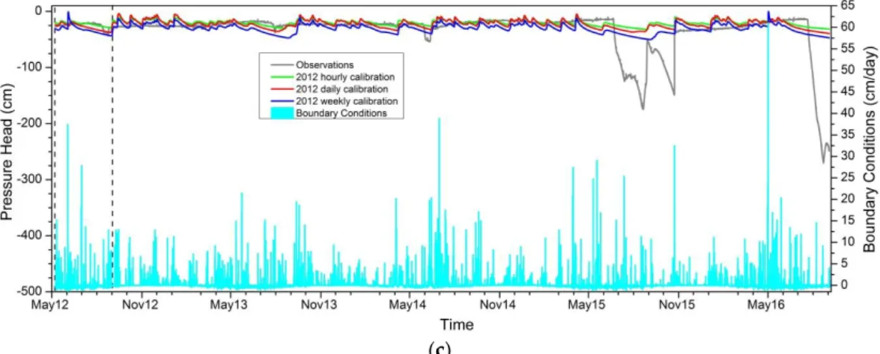
Figure 4. Pressure head values modeled for the period from May 2012 to September 2016. The model
is calibrated using hourly, daily, and weekly data for the period from June to September 2012 (limited by vertical straight lines): pressure head values at depths of 42 cm (a), 71 cm (b) and 116 cm (c).
(a)
(c)
Figure 5. Pressure head values modeled for the period from May 2012 to September 2016. The model
is calibrated using hourly, daily, and weekly data for the period from April to December 2015 (limited by vertical straight lines in the picture): pressure head values at depths of 42 cm (a), 71 cm (b), and 116 cm (c).
Simulations using 2012 calibrations do not show the offset observed when using the 2015 calibrations (Figure 4), but the peaks are not well reproduced. The −42 cm peaks are overestimated by the hourly and weekly calibrations, and the −71 cm and −116 cm peaks are underestimated by all calibrations. This may be related to the lack of dynamic and large depressions in the 2012 calibration data set. A strong impact of the 2012 calibration data frequency is seen for the simulated pressure head at a depth of 42 cm. No clear trend can be identified, but the weekly calibration leads to very large depressions (−12,000 cm), whereas the daily and hourly calibrations show smaller depressions (−1000 cm and −3000 cm). From this point of view, the numerical results obtained with the parameters coming from the 2012 weekly calibration are less realistic and quite different compared to the measurements.
The lowest impact of sample frequency on the calibration, which was observed for the 2015 data, may be related to higher variability in this dataset in the sense of higher information content. A less variable dataset is more likely influenced by the sample frequency, since it is more affected by each information loss.
3.4. Drained Flux
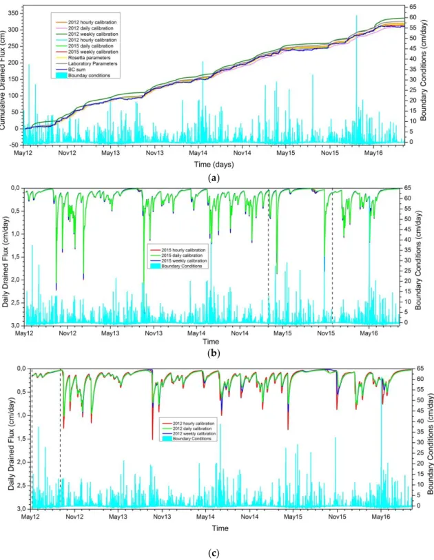
Modeling of the drained water flux at 150 cm depth is useful for evaluating aquifer recharge and water balance. Cumulative drained fluxes are strictly controlled by infiltration fluxes and thus by the boundary conditions. The cumulative drained flux curve is almost superimposed onto the cumulative boundary condition at the soils surface (Figure 6a). There was little calibration impact observed on the cumulative drained flux. Only the 2012 weekly calibration results in a deviated curve, but this calibration has the largest uncertainty on the parameters (Table 3). Comparing the cumulative drained flux to the imposed top boundary condition shows that the average relative error is less than 1% using the 2015 calibrated parameters; this average relative difference is greater for the 2012 calibrated parameters with a maximum of over 15% for the weekly frequency. An impact can be noticed on the instant drained flux, which is not on its dynamic but on its peak amplitude. The 2015 calibrations show approximately 50% higher peaks, and there is almost no calibration impact of the sampling frequency. A larger sampling frequency impact is observed using the 2012 calibrations, which shows higher peaks for the hourly sampling.
(a)
(b)
(c)
Figure 6. Modeled cumulative (a) and daily (b and c) drained flux at the depth of 150 cm for the
period from May 2012 to September 2016. The model is calibrated using hourly, daily, and weekly data for the periods from April to December 2015 (b) and from June to September 2012 (c) (calibration period is limited by vertical straight lines on each picture).
The modeling of drained flux is therefore hardly influenced by the sampling frequency of the calibration data or the choice of the calibration period. The influence of the calibration on the drained flux is relevant only for peak heights. As previously observed for the pressure head, the 2015 calibrations are less influenced by the sampling frequency due to their higher effectiveness.
The water saturation of each layer, which is computed using Equation (17), provides information about the water quantity contained in the soil porosity. The saturation level for each layer is estimated as follows:
,
1 , ,
Lj Nn i r Lj Lj i s Lj r Lj SL (17)where SLLj refers to the saturation level of the jth layer [-] and NnLj is the number of nodes in layer j.
Small effects from the sampling frequency on the saturation level simulations are seen for the 2015 calibrations (Figure 7a). Only daily sampling provides a larger saturation level than the hourly and weekly sampling for a third layer.
(a)
(b)
Figure 7. Saturation level modeled for the period from May 2012 to September 2016 for a three-layer
model. The model is calibrated using hourly, daily and weekly data for the periods from April to December 2015 (a) and from June to September 2012 (b) (calibration period is limited by vertical straight lines on each picture).
A larger effect is observed for the 2012 calibrations, except for the first layer saturation level (Figure 7b). Weekly sampling provides a larger saturation level for the second layer. The third layer saturation level increases passing from hourly to weekly and back to daily sampling.
Both 2012 and 2015 calibrations result in an unlikely, very humid first layer; its mean saturation is greater than 95% during the entire period. This is probably related to the clay-like small ‚n‛ values of the first layer obtained for all calibrations. Inversely, the mean saturation level of layers 2 and 3 are smaller than 25% for the 2015 calibration period due to the larger values of ‚n‛ and Ksat.
4. Conclusions
Soil hydraulic parameters are of great importance in the numerical modeling of vadose zone processes. Their measurement or determination throughout laboratory experiments or in situ tests is usually invasive, destructive, and often inappropriate for the model definition and scales. Since the simulated pressure heads at different depths agree well with the monitored data over a period of five years, this study demonstrates that the inverse modeling approach provides an interesting and efficient way to assess soil parameters.
The first step to emphasize is the great attention dedicated to boundary conditions, which is suggested in the literature. Based on this, we have deduced that the BILJOU software provides a good estimation of the AET. Precipitation monitored near the soil profile should be reduced to 80% to avoid overestimation of the soil humidity. This difficulty, which is potentially linked to the topography and aerodynamic effects, has also been mentioned in the literature [34]. Contrary to other experimental sites where the bottom boundary condition is also monitored, we assumed a free drainage condition.
Sample analyses allowed us to propose a consistent discretization of the domain in 3 layers. Even if the first two MP sensors could not be included in our inverse modeling approach due to incoherent results in regards to the top BC, data from the 3 Campbell 257 (Watermark) devices at depths of 42 cm, 71 cm, and 116 cm have been stored every 10 min between 2011 and 2016. Temperature correction has been implemented to prevent perturbations, which was as advised in the instruction manual and previous studies [43,64]. Because of its internal gypsum tablet, the sensor was not sensitive to the soil bulk electroconductivity. This type of sensor generally required polynomial calibration relationships or better still, field calibration curves [64]. The accuracy of the measurement can also be correlated to the soil saturation level, which suggests adopting various models for the calibration curves [65]. Nonetheless, Watermark users generally investigated a first relationship to estimate the MP and then converted its value into water content through a logarithmic equation or a power function (van Genuchten model). Our approach was quite different because no other control measurements were available in the vertical profile, which prevented field calibration. In addition, the use of a quadratic function was not successful. Finally, the van-Genuchten model was implied for the inverse parameters estimation instead of into the sensor calibration. In the context of field studies in natural (not controlled) environment, the results depicted in this paper clearly illustrated both the originality and efficiency of our approach.
McCann et al. [45] and Thompson et al. [65] discussed the limitations displayed by the Watermark sensor in case of rapidly drying media or very moist soil. Varble and Chávez [64] also suggested that the energy state of the water into the sensor must equilibrate with that of the surrounding soil. The higher discrepancy between measurements and simulations in the deeper layers, which have a higher content of sand and could drain water faster, may be explained in the abovementioned point. In addition, the saturation level of the deeper layers is less. In fact, more fluctuations were observed in the numerical results because the sensors have perhaps encountered limitations due to the dynamic effect. Thompson et al. [65] indicated that no clear advantage was obtained by using continuously collected data (2 times per hour) compared to using single daily data points. This remark noted for calibration investigations joins the results of our study on the impact of the measurement frequency used in the inverse problem. Hydraulic parameters obtained using daily sampled data led to very accurate results. Nevertheless, these authors also claimed to include dynamic datasets because of the constantly changing field conditions. As shown by comparing two calibration periods, our results agree with the necessity of selecting measurements that can reflect the range of variations in the field conditions.
Concerning the parameters estimation using the inverse modeling approach, our objective was to use the MP measurements to estimate 3 hydraulic parameters of the Mualem-van Genuchten model (Ksat, n, α) for each of the three layers. This goal is consistent with what appeared in the
literature (see [66–69]). Estimating the water content at saturation would have required the collection of additional data, which was done in other studies [70–72]. Nonetheless, we underline that the
present exercise was challenging due to a range of variations in the MP measurements, which were quite extensive compared to the cases generally presented that dealt with (field) data monitoring.
The best direct simulation over the 2012–2016 period is the one performed using the 2015 daily calibrated parameters (according to RMSE and ME), although the best parameter optimizations (according to AIC, BIC, and RMSE) are those related to the 2012 period. The 2015 daily calibrated parameters more efficiently reproduce the observed dynamic and extreme events. Nonetheless, the means bias errors indicate that the ROSETTA computer program provides a parameter set that allows for the efficient description of the trend of measured data.
In this study, the importance of the choice of calibration period clearly emerges. A dataset with high variability is suitable, and should include a recording frequency apt to describe the dynamic of the measured physical variables. The 2015 pressure head measurements show high variability and thus bring ‚more information‛ to the calibration process. Consequently, the model calibrations performed using 2015 data are more stable and less influenced by the frequency of data sampling. In contrast, the 2012 data set shows low variability, model calibrations performed using 2012 data are heavily influenced by the frequency of data sampling, and optimized parameters show larger errors. An interesting issue in this study is that once a good period of calibration is chosen, the influence of the sampling frequency is minor, at least under our conditions. This means that data acquisition using a weekly frequency could be sufficient to estimate the drainage flux and thus the aquifer recharge. If this issue is confirmed, weekly sampling could allow for an optimization of financial and human resources in the environmental observatories. To add to what has been stated previously, diversifying the sensors is certainly an interesting means for accessing other parameters or monitoring other sites.
Finally, several reasons may explain the discrepancy between the measured and simulated MP: (i) Water content values have not been monitored, which probably left uncertainty in the soil hydraulic properties; (ii) Hysteresis has been omitted in this study, whereas the wetting and drying processes are followed by one another in the field environment; (iii) The bottom boundary condition was not monitored and the modeling approach contained part of the uncertainty; and (iv) Since the rainfall measurement was not determined directly near the vertical profile, the top boundary condition has been estimated as the difference between 80% rainfall and the AET obtained using the BILJOU software. The results presented in this article will be the basis for future investigations, and the abovementioned points could improve our modeling of the catchment.
Acknowledgments: The study was partially financed by Strasbourg University and by the French Agence
Nationale de la Recherche through the project Hydrocrizsto (HYDRO-Geochemical behavior of Critical Zone at Strengbach Observatory, http://hydrocrizsto.unistra.fr/). The authors are grateful to S. Benarioumlil and P. Friedmann for their help installing the devices and data recovery. We would like also to extend great thanks to M.C. Pierret for her constant help, advice and enthusiasm.
Author Contributions: Ivan Toloni and Philippe Ackerer contributed to the numerical simulations and
analyses; they also actively worked on the writing of this paper. Solenn Cotel and Daniel Viville participated in the device installations for the vertical profile in the Strengbach catchment; they provided the different data used in this study and were very involved in the field monitoring. François Lehmann and Benjamin Belfort contributed substantially to many different steps in this project, which included field devices installation, numerical modeling developments, simulations analysis, and reaction to the present article.
Conflicts of Interest: The authors declare no conflict of interest.
References
1. Pachauri, R.K.; Allen, M.R.; Barros, V.R.; Broome, J.; Cramer, W.; Christ, R.; Church, J.A.; Clarke, L.; Dahe, Q.; Dasgupta, P. Climate Change 2014: Synthesis Report. Contribution of Working Groups I, II and III to the fifth
Assessment Report of the Intergovernmental Panel on Climate Change; IPCC: Geneva, Switzerland, 2014;
2. Guo, L.; Lin, H. Critical Zone Research and Observatories: Current Status and Future Perspectives. Vadose
3. Javaux, M.; Couvreur, V.; Vanderborght, J.; Vereecken, H. Root Water Uptake: From Three-Dimensional Biophysical Processes to Macroscopic Modeling Approaches. Vadose Zone J. 2013, 12, doi:10.2136/vzj2013.02.0042.
4. Llorens, P.; Domingo, F. Rainfall partitioning by vegetation under Mediterranean conditions. A review of studies in Europe. J. Hydrol. 2007, 335, 37–54.
5. Muzylo, A.; Llorens, P.; Valente, F.; Keizer, J.J.; Domingo, F.; Gash, J.H.C. A review of rainfall interception modelling. J. Hydrol. 2009, 370, 191–206.
6. Rodriguez-Iturbe, I.; D’Odorico, P.; Porporato, A.; Ridolfi, L. On the spatial and temporal links between vegetation, climate, and soil moisture. Water Resour. Res. 1999, 35, 3709–3722.
7. Maxwell, R.M.; Putti, M.; Meyerhoff, S.; Delfs, J.-O.; Ferguson, I.M.; Ivanov, V.; Kim, J.; Kolditz, O.; Kollet, S.J.; Kumar, M. Surface-subsurface model intercomparison: A first set of benchmark results to diagnose integrated hydrology and feedbacks. Water Resour. Res. 2014, 50, 1531–1549.
8. Kollet, S.; Sulis, M.; Maxwell, R.M.; Paniconi, C.; Putti, M.; Bertoldi, G.; Coon, E.T.; Cordano, E.; Endrizzi, S.; Kikinzon, E. The integrated hydrologic model intercomparison project, IH-MIP2: A second set of benchmark results to diagnose integrated hydrology and feedbacks. Water Resour. Res. 2017, 53, 867–890. 9. Seneviratne, S.I.; Corti, T.; Davin, E.L.; Hirschi, M.; Jaeger, E.B.; Lehner, I.; Orlowsky, B.; Teuling, A.J.
Investigating soil moisture–climate interactions in a changing climate: A review. Earth-Sci. Rev. 2010, 99, 125–161.
10. Dorigo, W.A.; Wagner, W.; Hohensinn, R.; Hahn, S.; Paulik, C.; Xaver, A.; Gruber, A.; Drusch, M.; Mecklenburg, S.; van Oevelen, P.; et al. The International Soil Moisture Network: A data hosting facility for global in situ soil moisture measurements. Hydrol. Earth Syst. Sci. 2011, 15, 1675–1698.
11. Liu, Y.Y.; Parinussa, R.M.; Dorigo, W.A.; De Jeu, R.A.M.; Wagner, W.; van Dijk, A.I.J.M.; McCabe, M.F.; Evans, J.P. Developing an improved soil moisture dataset by blending passive and active microwave satellite-based retrievals. Hydrol. Earth Syst. Sci. 2011, 15, 425–436.
12. Lee, H.J. Sequential Ensembles Tolerant to Synthetic Aperture Radar (SAR) Soil Moisture Retrieval Errors.
Geosciences 2016, 6, 19, doi:10.3390/geosciences6020019.
13. Pérez Hoyos, C.I.; Krakauer, Y.N.; Khanbilvardi, R.; Armstrong, A.R. A Review of Advances in the Identification and Characterization of Groundwater Dependent Ecosystems Using Geospatial Technologies. Geosciences 2016, 6, 17, doi:10.3390/geosciences6020017.
14. Vereecken, H.; Schnepf, A.; Hopmans, J.W.; Javaux, M.; Or, D.; Roose, T.; Vanderborght, J.; Young, M.H.; Amelung, W.; Aitkenhead, M.; et al. Modeling Soil Processes: Review, Key Challenges, and New Perspectives. Vadose Zone J. 2016, 15, 1–57.
15. Albergel, C.; Rüdiger, C.; Pellarin, T.; Calvet, J.-C.; Fritz, N.; Froissard, F.; Suquia, D.; Petitpa, A.; Piguet, B.; Martin, E. From near-surface to root-zone soil moisture using an exponential filter: An assessment of the method based on in-situ observations and model simulations. Hydrol. Earth Syst. Sci. 2008, 12, 1323–1337. 16. Vereecken, H.; Huisman, J.A.; Bogena, H.; Vanderborght, J.; Vrugt, J.A.; Hopmans, J.W. On the value of
soil moisture measurements in vadose zone hydrology: A review. Water Resour. Res. 2008, 44, doi:10.1029/2008WR006829.
17. Ochsner, T.E.; Cosh, M.H.; Cuenca, R.H.; Dorigo, W.A.; Draper, C.S.; Hagimoto, Y.; Kerr, Y.H.; Njoku, E.G.; Small, E.E.; Zreda, M.; et al. State of the Art in Large-Scale Soil Moisture Monitoring. Soil Sci. Soc. Am.
J. 2013, 77, 1888–1919.
18. Romano, N. Soil moisture at local scale: Measurements and simulations. J. Hydrol. 2014, 516, 6–20. 19. Susha Lekshmi, S.U.; Singh, D.N.; Shojaei Baghini, M. A critical review of soil moisture measurement.
Measurement 2014, 54, 92–105.
20. Robinson, D.A.; Campbell, C.S.; Hopmans, J.W.; Hornbuckle, B.K.; Jones, S.B.; Knight, R.; Ogden, F.; Selker, J.; Wendroth, O. Soil Moisture Measurement for Ecological and Hydrological Watershed-Scale Observatories: A Review. Vadose Zone J. 2008, 7, 358–389.
21. Assouline, S.; Or, D. Conceptual and Parametric Representation of Soil Hydraulic Properties: A Review.
Vadose Zone J. 2013, 12, 1–20.
22. Reynolds, W.D.; Bowman, B.T.; Brunke, R.R.; Drury, C.F.; Tan, C.S. Comparison of Tension Infiltrometer, Pressure Infiltrometer, and Soil Core Estimates of Saturated Hydraulic Conductivity. Soil Sci. Soc. Am. J.
2000, 64, 478–484.
23. Pachepsky, Y.; Rawls, W.J.; Giménez, D. Comparison of soil water retention at field and laboratory scales.
24. Vrugt, J.A.; Stauffer, P.H.; Wöhling, T.; Robinson, B.A.; Vesselinov, V.V. Inverse Modeling of Subsurface Flow and Transport Properties: A Review with New Developments. Vadose Zone J. 2008, 7, 843–864. 25. Jacques, D.; Šimůnek, J.; Timmerman, A.; Feyen, J. Calibration of Richards’ and convection–dispersion
equations to field-scale water flow and solute transport under rainfall conditions. J. Hydrol. 2002, 259, 15–31. 26. Ritter, A.; Hupet, F.; Muñoz-Carpena, R.; Lambot, S.; Vanclooster, M. Using inverse methods for
estimating soil hydraulic properties from field data as an alternative to direct methods. Agric. Water
Manag. 2003, 59, 77–96.
27. Ritter, A.; Muñoz-Carpena, R.; Regalado, C.M.; Vanclooster, M.; Lambot, S. Analysis of alternative measurement strategies for the inverse optimization of the hydraulic properties of a volcanic soil. J. Hydrol.
2004, 295, 124–139.
28. Ireson, A.M.; Wheater, H.S.; Butler, A.P.; Mathias, S.A.; Finch, J.; Cooper, J.D. Hydrological processes in the Chalk unsaturated zone—Insights from an intensive field monitoring programme. J. Hydrol. 2006, 330, 29–43.
29. Wollschläger, U.; Pfaff, T.; Roth, K. Field-scale apparent hydraulic parameterisation obtained from TDR time series and inverse modelling. Hydrol. Earth Syst. Sci. 2009, 13, 1953–1966.
30. Scharnagl, B.; Vrugt, J.A.; Vereecken, H.; Herbst, M. Inverse modelling of in situ soil water dynamics: Investigating the effect of different prior distributions of the soil hydraulic parameters. Hydrol. Earth Syst.
Sci. 2011, 15, 3043–3059.
31. Andreasen, M.; Andreasen, L.A.; Jensen, K.H.; Sonnenborg, T.O.; Bircher, S. Estimation of Regional Groundwater Recharge Using Data from a Distributed Soil Moisture Network. Vadose Zone J. 2013, 12, doi:10.2136/vzj2013.01.0035.
32. Mathias, S.A.; Sorensen, J.P.R.; Butler, A.P. Soil moisture data as a constraint for groundwater recharge estimation. J. Hydrol. 2017, 552, 258–266.
33. Thoma, M.J.; Barrash, W.; Cardiff, M.; Bradford, J.; Mead, J. Estimating Unsaturated Hydraulic Functions for Coarse Sediment from a Field-Scale Infiltration Experiment. Vadose Zone J. 2014, 13, 1–17.
34. Seki, K.; Ackerer, P.; Lehmann, F. Sequential estimation of hydraulic parameters in layered soil using limited data. Geoderma 2015, 247–248, 117–128.
35. Singh, S K.; Ibbitt, R.; Srinivasan, M.S.; Shankar, U. Inter-comparison of experimental catchment data and hydrological modelling. J. Hydrol. 2017, 550, 1–11.
36. Brocca, L.; Tullo, T.; Melone, F.; Moramarco, T.; Morbidelli, R. Catchment scale soil moisture spatial– temporal variability. J. Hydrol. 2012, 422–423, 63–75.
37. Hawke, R.; McConchie, J. In situ measurement of soil moisture and pore-water pressures in an ‘incipient’ landslide: Lake Tutira, New Zealand. J. Environ. Manag. 2011, 92, 266–274.
38. Ackerer, J.; Chabaux, F.; Van der Woerd, J.; Viville, D.; Pelt, E.; Kali, E.; Lerouge, C.; Ackerer, P.; di Chiara Roupert, R.; Négrel, P. Regolith evolution on the millennial timescale from combined U–Th–Ra isotopes and in situ cosmogenic 10Be analysis in a weathering profile (Strengbach catchment, France). Earth Planet.
Sci. Lett. 2016, 453, 33–43.
39. Weill, S.; Delay, F.; Pan, Y.; Ackerer, P. A low-dimensional subsurface model for saturated and unsaturated flow processes: Ability to address heterogeneity. Comput. Geosci. 2017, 21, 301–314.
40. Gangloff, S.; Stille, P.; Schmitt, A.-D.; Chabaux, F. Factors controlling the chemical composition of colloidal and dissolved fractions in soil solutions and the mobility of trace elements in soils. Geochim. Cosmochim.
Acta 2016, 189, 37–57.
41. Beaulieu, E.; Lucas, Y.; Viville, D.; Chabaux, F.; Ackerer, P.; Goddéris, Y.; Pierret, M.-C. Hydrological and vegetation response to climate change in a forested mountainous catchment. Model. Earth Syst. Environ.
2016, 2, 191, doi:10.1007/s40808-016-0244-1.
42. Pierret, M.C.; Stille, P.; Prunier, J.; Viville, D.; Chabaux, F. Chemical and U–Sr isotopic variations in stream and source waters of the Strengbach watershed (Vosges mountains, France). Hydrol. Earth Syst. Sci. 2014,
18, 3969–3985.
43. Campbell Scientific. Instruction Manual: Models 253-L and 257-L Soil Matric Potential Sensors; Révision: 9/13; Campbell Scientific, Inc.: Logan, UT, USA, 2013;
44. Shock, C.C.; Barnum, J.M.; Seddigh, M. Calibration of Watermark Soil Moisture Sensors for Irrigation Management. In Proceedings of the International Irrigation Show; Irrigation Association: San Diego California, CA, USA, 1998; pp. 139–146.