Developing Clinically Useful Risk Stratification
Models
by
Paul Daniel Myers
B.S.E., University of Michigan (2015)
S.M., Massachusetts Institute of Technology (2017)
Submitted to the Department of Electrical Engineering and Computer
Science
in partial fulfillment of the requirements for the degree of
Doctor of Philosophy
at the
MASSACHUSETTS INSTITUTE OF TECHNOLOGY
September 2020
c
○ Massachusetts Institute of Technology 2020. All rights reserved.
Author . . . .
Department of Electrical Engineering and Computer Science
August 28, 2020
Certified by . . . .
Collin M. Stultz
Professor of Electrical Engineering and Computer Science
Thesis Supervisor
Accepted by . . . .
Leslie A. Kolodziejski
Professor of Electrical Engineering and Computer Science
Chair, Department Committee on Graduate Students
Developing Clinically Useful Risk Stratification Models
by
Paul Daniel Myers
Submitted to the Department of Electrical Engineering and Computer Science on August 28, 2020, in partial fulfillment of the
requirements for the degree of Doctor of Philosophy
Abstract
When a patient presents to a hospital with symptoms of cardiovascular disease, one of the first courses of action is to estimate the patient’s risk of an adverse outcome. The process of categorizing patients by risk level, known as risk stratification, is an essential step in assigning appropriate therapy. Risk stratification models, which aid clinicians in this task, consist of feature sets that are combined by an algorithm to yield a score. In addition to the performance of the model, a key factor in model de-velopment is clinician acceptance of the score. One way to bolster clinician acceptance is to choose parsimonious feature sets to be used in risk scores that are convenient to integrate into the clinical workflow. A second consideration is establishing clinician trust in the model predictions. This is particularly important when using models that are difficult to explain to clinicians and when it is not straightforward to iden-tify failure modes for the model. Providing clinicians with a measure of how much to trust a given prediction from a model is one way to encourage the use of models that are difficult to interpret. In this thesis, we consider the problem of developing clinically useful risk models using real clinical data. We begin by discussing how to choose clinical variables in a data-driven fashion in the context of acute coronary syn-drome. We present a risk score that can accommodate a variable number of inputs and demonstrate that it has superior performance to the Global Registry of Acute Coronary Events (GRACE) risk score, particularly on the difficult to risk stratify low-risk patients (AUC 0.754 vs. 0.688 for the GRACE score, p < 0.007). We then discuss the development of a risk score for aortic stenosis (AS) using both data-driven feature selection and expert opinion. We show that the model performs well on pa-tients with moderate to severe aortic stenosis (AUC 0.74), as well as on the difficult to risk stratify low gradient severe AS subgroup (2-5 year hazard ratios ≥ 3.3, p < 0.05). Finally, we develop a method to identify unreliable predictions in clinical risk models and show, using the GRACE dataset, that we can identify subgroups of poor model performance to aid in bolstering clinician trust of risk models.
Thesis Supervisor: Collin M. Stultz
Acknowledgments
I am indebted to my thesis advisor, Collin Stultz, for his patience, encouragement, and guidance. My time in graduate school was filled with challenges and I cannot imagine having completed the course without Collin’s support in both the technical and non-technical aspects of the process.
I am also grateful to the thesis committee members John Guttag and Peter Szolovits. John provided indispensable feedback throughout the years, as well as many opportunities to learn to speak in front of a group and field difficult questions. Peter provided important input on the final drafts of the thesis and was instrumental in preparing for the defense.
I would also like to acknowledge the members of the Computational Cardiovascu-lar Research Group, Wangzhi Dai, Daphne Schlesinger, Aniruddh Raghu, Katherine Young, Erik Reinertsen, Megumi Masuda-Loos, and Arlene Wint, for their fellowship and feedback.
Finally, I would like to thank my family for their support throughout the years. Although not physically present with me during this thesis work, they nonetheless shouldered much of the burden along with me. I would also like to thank Fr. John Downie and Presbytera Camelia for their kindness, as well as Harris and Jessica Pitsillides. I will never be able to thank them adequately for what they have done for me. Thanks are also due to Fr. Asterios Gerostergios (+2019) and Venkat Arun.
Contents
1 Introduction 19
1.1 Background . . . 21
1.1.1 Acute Coronary Syndrome . . . 21
1.1.2 Aortic Stenosis . . . 27
1.2 Organization of the Thesis . . . 30
1.2.1 Choosing Clinical Variables for Patient Risk Stratification Post-Acute Coronary Syndrome . . . 30
1.2.2 Prediction of Outcomes in Patients with Aortic Stenosis Using Machine Learning . . . 31
1.2.3 Identifying Unreliable Predictions in Clinical Risk Models. . . 33
2 Choosing Clinical Variables for Risk Stratification Post-Acute Coro-nary Syndrome 35 2.1 Methods . . . 36
2.1.1 Feature Selection with Bootstrap Lasso Regression . . . 36
2.1.2 Model Development and Testing. . . 38
2.1.3 Data Imputation . . . 39
2.1.4 Testing on the Validation Set . . . 40
2.1.5 Statistical Analyses . . . 41
2.2 Results . . . 41
2.2.1 Features Selection with BLR . . . 41
2.2.3 Evaluating the Relative Importance of Non-GRACE Score
Fea-tures . . . 42
2.2.4 RLRVI Discriminatory Ability Using a Subset of Clinical Features 42 2.2.5 RLRVI Performance on the Validation Set . . . 43
2.3 Discussion . . . 46
3 Predicting Outcomes in Patients with Aortic Stenosis Using Machine Learning 53 3.1 Methods . . . 54
3.1.1 Primary Cohort . . . 54
3.1.2 Data Preprocessing . . . 54
3.1.3 Feature Selection . . . 55
3.1.4 AS Risk Stratification (ASRS) Model . . . 56
3.1.5 Validation Cohort . . . 58
3.1.6 Baseline Risk Model . . . 59
3.1.7 Ethics Approval . . . 59 3.2 Results . . . 59 3.2.1 Primary Cohort . . . 59 3.2.2 Validation Cohort . . . 62 3.3 Discussion . . . 64 3.3.1 Clinical Interface . . . 67 3.3.2 Limitations . . . 67 3.4 Conclusions . . . 68
4 Identifying Unreliable Predictions in Clinical Risk Models 69 4.1 Methods . . . 72
4.1.1 A Method for Estimating Unreliable Predictions . . . 72
4.1.2 Clinical Risk Models and Data. . . 75
4.1.3 Calculating 𝑈 (⃗𝑥) . . . 77
4.1.4 Trust Score Calculations . . . 79
4.2 Results . . . 80
4.2.1 Prediction Unreliability is a Function of Class Imbalance . . . 80
4.2.2 Performance of the GRACE Score in an Unreliable Subgroup . 81 4.2.3 The Most Unreliable GRACE Predictions Have Significantly Reduced Performance. . . 83
4.2.4 Unreliable Predictions in a Stroke Risk Model . . . 86
4.3 Discussion . . . 87
5 Summary and Conclusion 95 5.1 Choosing Variables for Risk Stratification Post-Acute Coronary Syn-drome . . . 95
5.1.1 Implications for Future Work . . . 96
5.2 Predicting Outcomes in Aortic Stenosis . . . 96
5.2.1 Implications for Future Work . . . 97
5.3 Identifying Unreliable Predictions in Clinical Risk Models . . . 97
5.3.1 Implications for Future Work . . . 98
A Additional Experiments for the Unreliability Metric of Chapter 4 99 A.1 Application of the Unreliability Score to the Aortic Stenosis Risk Score 99 A.2 Further Considerations: Addressing Unreliable Predictions . . . 100
A.2.1 Oversampling Unreliable Predictions . . . 100
List of Figures
1-1 (a) Anatomy of a normal heart [41] and (b) a heart with AS with observable left ventricular hypertrophy [42]. . . 27
1-2 AS of increasing severity [42]. . . 28
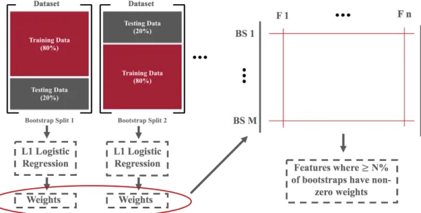
2-1 Schematic of the BLR algorithm. The dataset is first partitioned into 𝑀 training and testing sets by stratified sampling with replacement. Separate L1-regularized logistic regression models are trained on each training set and the 𝑛 feature weights are compiled. Features that appear in at least 𝑁 % of the bootstrap splits are retained for further model development. . . 37
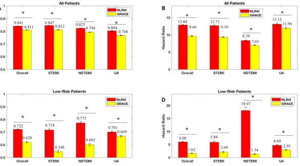
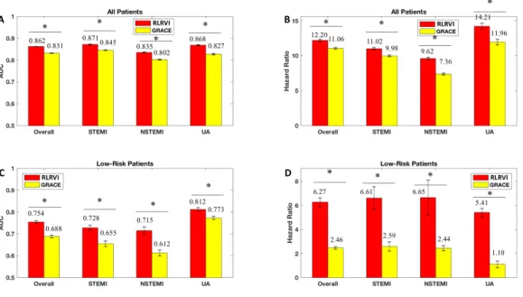
2-2 RLR Performance on the Development Set. AUCs and six-month haz-ard ratios in the overall (a,b) and low-risk (GRACE < 87) subset (c,d) of the development set. Error bars show one standard error of the mean. * indicates p < 0.001. Numbers above the bars indicate mean values. AUC = area under the curve; GRACE = Global Registry of Acute Coronary Events; RLRVI = ridge logistic regression with vari-able inputs; STEMI = ST elevation myocardial infarction; NSTEMI = non-ST elevation myocardial infarction; UA = unstable angina. . . . 45
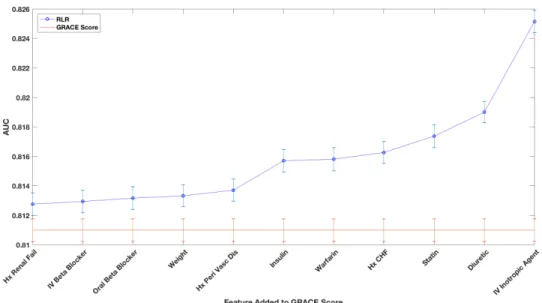
2-3 Evaluating the Relative Importance of non-GRACE Score Features. AUCs from adding one of the 11 non-GRACE score features at a time and imputing the remaining features. AUCs are averaged over 100 bootstrapped test sets. Error bars show one standard error of the mean. All models show improved performance over the GRACE score with p< 0.001. AUC = area under the curve; GRACE = Global Registry of Acute Coronary Events; RLRVI = ridge logistic regression with variable inputs; Hx = History; Peri Vasc Dis = peripheral vascular disease; IV = intravenous; CHF = congestive heart failure. . . 46
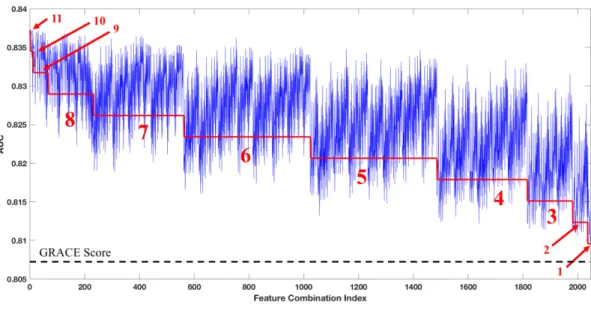
2-4 RLRVI Discriminatory Ability Using a Subset of Clinical Features. AUCs averaged over 10 bootstrap splits of the development set for all possible combinations of the 11 non-GRACE score features selected by BLR. The red line and numbers indicate the number of features that were known and therefore not imputed. For example, the red 6 indi-cates that all points in that range were generated by models that had six of the non-GRACE score features available; all possible combina-tions of 11 choose 6 are represented in this range. The performance of the GRACE score on the same 10 bootstrap splits is shown by the dashed line at the bottom of the plot. All feature combinations show improvement over the GRACE score with p < 0.003. AUC = area under the curve; GRACE = Global Registry of Acute Coronary Event. 47
2-5 RLRVI Performance on the Validation Set. AUCs and six-month haz-ard ratios in the overall (a,b) and low-risk (GRACE < 87) subset (c,d) of the validation set. Error bars show one standard error of the mean. * indicates p < 0.007. Numbers above the bars indicate mean val-ues. AUC = area under the curve; GRACE = Global Registry of Acute Coronary Events; RLRVI = ridge logistic regression with vari-able inputs; STEMI = ST elevation myocardial infarction; NSTEMI = non-ST elevation myocardial infarction; UA = unstable angina. . . . 48
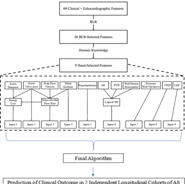
3-1 Flowchart describing feature selection and model construction. Ab-breviations: AS: aortic stenosis; CHF: congestive heart failure; CKD: chronic kidney disease; LGAS: low-gradient aortic stenosis; MI: my-ocardial infarction; PVD: peripheral vascular disease. . . 57
3-2 Time to event analysis based on ASRS model in aortic stenosis patients within (a) the primary cohort, (b) the LGAS subgroup of the primary cohort, and (c) the group of patients not undergoing intervention in the primary cohort. High-risk group determined by upper quartile of ranked risk. Curves are averaged over 10 bootstrapped test sets. . . . 63
3-3 Time to event analysis based on ASRS model in aortic stenosis patients within (a) the validation cohort, (b) the LGAS subgroup of the valida-tion cohort, and (c) the group of patients not undergoing intervenvalida-tion in the validation cohort. High-risk group determined by upper quartile of ranked risk. . . 65
4-1 Unreliability scores are a function of class imbalance. (a) Average un-reliability as a function of the classifier prediction, 𝑓 (⃗𝑥), when there is no class imbalance in the data, 𝑃 (𝑦 = 1) = 0.05. (b) Average un-reliability for different predictions, 𝑓 (⃗𝑥), in the setting of large class imbalance, 𝑃 (𝑦 = 1) = 0.01. Calculated expected values assume a uniform distribution for 𝛽⃗𝑥. . . 81
4-2 Average pairwise distance between features of patients who fall within the top 1% of uncertainty and those that fall within the remainder of the dataset. Patients who have predictions that fall within the highest 1% of uncertainty form a set that has features that are at least as heterogeneous as the set containing patients who are not in this subgroup. 82
4-3 Prediction scores in the upper 50th percentile of unreliability (top 50% of 𝑈 (⃗𝑥) values) have worse performance. (a) Calibration curves (red -top 50%, black - bottom 50%), (b) Normalized Brier scores (inset shows expanded region corresponding to 0.89 ≤ Brier/Brier𝑛𝑢𝑙𝑙 ≤ 0.912), and
(c) Average AUCs for predicting the outcome of all-cause death within 6 months of presentation for predictions in the upper 50th percentile (red) and those within the lower 50th percentile (black). *p < 0.05; **p << 0.0001. Error bars are from 100 bootstrap splits and show one standard deviation (a) or one standard error of the mean (b and c). . 84
4-4 The most unreliable predictions (predictions within the top 1% of 𝑈 (⃗𝑥) values) in the GRACE risk model are associated worse performance. (a) Calibration curves (red - top 1%, black - bottom 99%), (b) nor-malized Brier scores, and (c) AUCs for the most unreliable predictions (red) and those that fall within the bottom 99% of 𝑈 (⃗𝑥) values (black). **p << 0.0001. Error bars are from 100 bootstrap splits and show one standard deviation (a) or one standard error of the mean (b and c). Error bars are truncated at 1. . . 84
4-5 Untrustworthy predictions in the GRACE risk model using the trust score. (a) Calibration curves (red - bottom 1%, black - top 99%), (b) normalized Brier scores, and (c) AUCs for the most untrustworthy predictions (red) and those that fall within the bottom 99% trust score values (black). Error bars are from 100 bootstrap splits and show one standard deviation (a) or one standard error of the mean (b and c). Error bars are truncated at 1. . . 85
4-6 Unreliable predictions in the Stroke risk model. (a) Calibration curves (red - top 1%, black - bottom 99%), (b) normalized Brier scores (in-set shows expanded region corresponding to 0.95 ≤ Brier/Brier𝑛𝑢𝑙𝑙 ≤
1.02), and (c) AUCs for the most untrustworthy predictions (red) and those that fall within the bottom 99% 𝑈 (⃗𝑥) values (black). **p << 0.0001. Error bars are from 100 bootstrap splits and show one standard deviation (a) or one standard error of the mean (b and c). . . 87
4-7 Untrustworthy predictions in the Stroke risk model using the trust score. (a) Calibration curves (red - bottom 1%, black - top 99%), (b) normalized Brier scores (inset shows expanded region corresponding to 0.95 ≤ Brier/Brier𝑛𝑢𝑙𝑙≤ 1.0), and (c) AUCs for the most untrustworthy
predictions (red) and those that fall within the bottom 99% 𝑈 (⃗𝑥) values (black). *p < 0.05, **p << 0.0001. Error bars are from 100 bootstrap splits and show one standard deviation (a) or one standard error of the mean (b and c). . . 88
4-8 Relative prevalence of positive outcomes in patients in different co-horts, defined by their uncertainty score. Patients in cohorts with high uncertainty are more heterogeneous with respect to the outcome than patients who have lower uncertainty scores. Insets juxtapose the prevalence of positive and negative patients within relevant subgroups. 89
A-1 Untrustworthy predictions in the aortic stenosis risk score. (a) AUCs and (b) Normalized Brier scores in the bottom 90% of 𝑈 (⃗𝑥) and top 10% of 𝑈 (⃗𝑥). *p < 0.05. Error bars are from 10 bootstrap splits and show one standard error of the mean. . . 100
List of Tables
2.1 Features selected by the bootstrap lasso. GRACE = Global Registry of Acute Coronary Events; IV = intravenous.. . . 43
2.2 Population characteristics in the development and validation sets. Num-bers for continuous variables are presented as the median with the in-terquartile range in parentheses. GRACE = Global Registry of Acute Coronary Events; CABG = coronary artery bypass grafting; MI = my-ocardial infarction; PCI = percutaneous coronary intervention; TIA = transient ischemic attack; IV = intravenous; ACE = angiotensin con-verting enzyme. . . 45
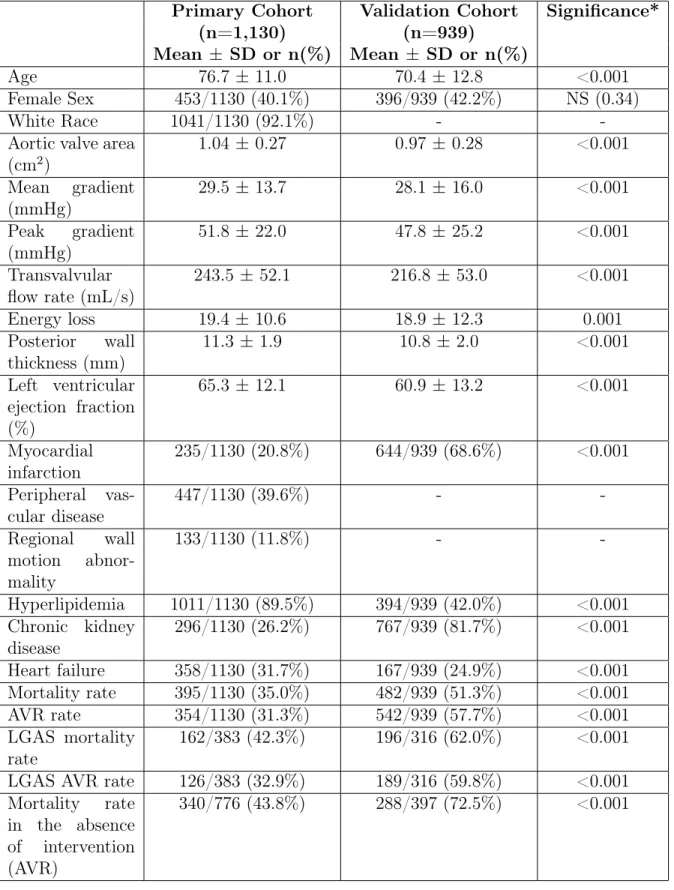
3.1 Descriptive Statistics. *Using Mann-Whitney U test and Chi-squared test, 2-sided significance. Abbreviations: AVR: aortic valve replace-ment; LGAS: low-gradient aortic stenosis. . . 60
3.2 Features selected in the final algorithm. *Calculated from aortic valve area, mean gradient and peak velocity using validated formula. **Cal-culated from aortic valve area, aortic sinus diameter and transvalvular flow rate using validated formula. ***Calculated from aortic valve area and aortic sinus diameter using validated formula; differs from feature 19 in that this feature does not use the transvalvular flow rate. . . . 61
3.3 Discriminatory ability of Baseline and ASRS risk models for the com-bined outcome of death/AVR in both the primary and Validation Co-horts. AUCs for the primary cohort are up to 7.3 years of follow and AUCs for the validation cohort are for up to 5 years of follow up. . . 62
3.4 Hazard ratios for death in the primary cohort, LGAS subset, and subset of patients in whom no intervention was performed.Results are from 10 bootstrapped test sets. Hazard ratios are calculated using the upper quartile of risk. Abbreviations: AS: aortic stenosis; AVR = aortic valve replacement; CI = confidence interval; HR = hazard ratio; LGAS: low-gradient aortic stenosis.. . . 64
3.5 Hazard ratios for death in the validation cohort, LGAS subset and pa-tients not undergoing intervention. Hazard ratios are calculated using the upper quartile of risk. Abbreviations: AS: aortic stenosis; AVR = aortic valve replacement; CI = confidence interval; HR = hazard ratio; LGAS: low-gradient aortic stenosis. . . 66
4.1 Population characteristics in the subset of the GRACE dataset used for all analyses. IDR: Interdecile range. . . 76
4.2 Characteristics of patients with predictions in the upper 1% of unreli-ability scores. IDR = interdecile range . . . 90
A.1 Results of applying oversampling to unreliable model predictions. STD = standard deviation.. . . 101
Chapter 1
Introduction
When a patient presents to a hospital with symptoms of cardiovascular disease, one of the first courses of action is to estimate the patient’s risk of an adverse outcome. The process of categorizing patients by risk level, known as risk stratification, is an essential step in assigning appropriate therapy. Invasive procedures, for example, are inappropriate for patients whose risk of future adverse events is lower than the risk of the procedure itself. Conversely, patients who are deemed to be very high risk might benefit from aggressive, higher risk strategies and closer follow-up [1,2].
Risk stratification models are constructed from various types of patient data, in-cluding demographics, medical history, physiological signals, and laboratory findings, which are all combined to yield a risk score. The choice of features to use in a risk model often arises from expert knowledge [3–5], data-driven approaches that auto-matically select a parsimonious feature set from a large list of available features [6], or some combination of the two [7,8]. Each approach is associated with its own set of advantages. Primarily expert-driven methods generally yield risk scores that are intuitive to clinicians, while primarily data-driven approaches might uncover features with prognostic value that were not previously considered to be important. Hybrid approaches offer some of the advantages of both extremes and are suitable in cases where it is important to capture clinical intuition while still allowing for the discovery previously unappreciated features that have prognostic value.
con-stituent features and the algorithm. It has been noted that if a sufficiently powerful feature set is available, complex models offer little or no advantage over simpler meth-ods such as logistic regression [9,10]. Indeed, clinical adoption of a risk score is often heavily dependent on not only its performance, but also how understandable it is to a clinician [10]. Basic logistic regression, for example, relates the odds ratio of the outcome of interest to a weighted, linear combination of the features. Given a set of features clinicians believe are important for predicting an outcome, it is easy to identify which features contribute most to the model’s predictions by looking at the feature weights. Thus, logistic regression is a popular choice for developing risk scores because its predictions are understandable to clinicians. Nonetheless, such models are limited in their flexibility; thus, there has been much recent interest in exploring more sophisticated methods based on machine learning that can take advantage of a range of data types [11–13]. Despite their impressive performance, however, the problem of clinician acceptance still remains. Indeed, it is often difficult to identify failure modes of sophisticated, “black box" models, making their safe deployment in a med-ical setting challenging [14]. An important step toward clinical adoption, then, is to develop methods that can identify when a model’s predictions should not be used. Such reliability checks can help bolster clinicians’ trust of a model, even when its inner workings cannot be easily understood.
In this thesis, we consider the problem of developing clinically useful risk mod-els. We begin by discussing an approach that uses limited a priori knowledge to select prognostic features, utilizing acute coronary syndrome as a model disease. We demonstrate with this approach that we can identify important features that were overlooked by experts when developing existing methods. We then turn to the prob-lem of combining expert opinion and data-driven feature selection to arrive at a risk score that contains both features that clinicians find intuitive and features that are not routinely considered in the context of aortic stenosis. We conclude by presenting a method to evaluate the reliability of clinical model predictions to aid in clinical adoption of risk models.
1.1
Background
As we use acute coronary syndrome and aortic stenosis as model diseases to develop our methods, we provide background here on their pathophysiology, as well as existing methods of risk stratification.
1.1.1
Acute Coronary Syndrome
The term acute coronary syndrome (ACS) refers to a spectrum of conditions that are primarily attributable to inadequate blood flow to the myocardium due to blockage of the coronary arteries [15]. ACS may be categorized based on how the electrocar-diogram (ECG), a non-invasive measurement of the electrical activity of the heart, is affected. Broadly, there are three categories of ACS: Non-ST segment elevation my-ocardial infarction (NSTEMI), ST segment elevation mymy-ocardial infarction (STEMI), and unstable angina (UA) [15]. In 2010, more than 1.1 million unique hospitalizations were ascribed to ACS and it is estimated that in the United States more than 780,000 people will experience an ACS each year [15,16].
Early risk-stratification plays an especially important role in the management of patients after an ACS. Patients who are identified as high risk using traditional risk metrics benefit from invasive therapies (such as percutaneous coronary intervention) within 24–48 hours of presentation [17,18]. A number of risk scores may be calculated using a patient’s presenting signs and symptoms, historical data - information that is available at the time of presentation – and the results of laboratory studies that can be obtained within minutes to hours after presentation [3,4,8]. Despite the relative success of these methods, an accurate assessment of patient risk remains a difficult task. Many risk scores, for example, fail to capture a significant number of deaths in certain patient cohorts [19,20]. Indeed, while patients who fall into the highest risk group have the highest prevalence of adverse outcomes, many adverse events occur in patients who are not classified as being high risk using conventional metrics. This happens because only a small fraction of the population is typically classified as being high risk by most risk scores. Although the probability of adverse outcomes in
patients who are not-high risk is relatively low, the absolute number of deaths in this cohort will be large as the vast majority of the population is considered to be not high-risk. Such “low risk-high number” phenomena plague many risk stratification problems in medicine [19,21]. There is therefore a great need to develop risk models that can more accurately identify high risk subgroups that are missed by traditional metrics.
Existing Risk Scores
A number of risk scores exist for ACS [22]. We review several here.
The TIMI Risk Scores Two Thrombolysis in Myocardial Infarction (TIMI) risk scores exist, one for NSTEMI/UA ACS [3] and one for STEMI ACS [23]. In designing the scores, ease of use by the clinician was a top priority: Neither score requires a specialized calculator, both use a small number of features (7 or 8), and both may be computed at presentation. Both scores were derived using multivariate regression.
The NSTEMI/UA score was designed to identify patients at high risk of all-cause mortality, new or recurrent MI, or severe recurrent ischemia requiring urgent revascularization up to 14 days after randomization and consists of the following seven features:
∙ Age ≥ 65
∙ ≥ 3 risk factors for coronary artery disease ∙ Prior coronary stenosis of ≥ 50
∙ ST-segment deviation on ECG at presentation ∙ ≥ 2 anginal events in prior 24 hours
∙ Use of aspirin in prior 7 days ∙ Elevated serum cardiac markers
In practice, the clinician counts the number of risk factors a given patient has, then converts the tally to a percent risk using a nomogram [3]. Each factor is worth one point.
The STEMI score was designed to identify patients at high risk of mortality within 30 days of presentation. It consists of the following eight features:
∙ Age ≥ 75 years (3 points) or age between 65 and 74 years (2 points) ∙ Systolic blood pressure < 100 mmHg (3 points)
∙ Heart rate > 100 beats per minute (2 points) ∙ Killip class II-IV (2 points)
∙ Anterior ST elevation or left bundle branch block (1 point) ∙ Diabetes, hypertension, or angina (1 point)
∙ Weight < 67 kg (1 point)
∙ Time to treatment > 4 hours (1 point)
As with the NTEMI/UA score, the STEMI score may be converted to a percent risk using a nomogram [23].
Although the TIMI risk scores offer the advantage of simplicity, they are limited in their ability to distinguish between high and low risk patients [22]. In particular, a high TIMI risk score has been shown to capture only 40% of the mortalities in a given cohort [24].
The GRACE Risk Score The Global Registry of Acute Coronary Events (GRACE) risk score was derived from a registry that was designed to reflect an unbiased and generalizable sample of ACS patients hospitalized from 1999 to 2007 in 94 hospitals in 14 countries [25]. Of the more than 1,000 variables in the registry, 198 are available within the critical first 24 hours of presentation [6]. Of these 198 variables, approxi-mately 50 were chosen by domain experts as inputs for stepwise feature selection, the
output of which was then further refined using expert knowledge to arrive at a final set of eight [7]. The eight features are the following:
∙ Age ∙ Pulse rate
∙ Systolic blood pressure ∙ Initial creatinine ∙ Killip class
∙ Cardiac arrest at presentation ∙ Initial positive cardiac enzymes ∙ ST-segment deviation at presentation
Unlike the TIMI scores, the GRACE score requires that the eight features be input to a specialized calculator, which is available online and as a smartphone app. The outcome of interest is all-cause mortality from admission to six months post-discharge. The final model utilized Cox proportional hazards regression and the direct output of the model is a raw score, which may be converted to a percent risk using a published nomogram [26].
Although the GRACE score requires a specialized calculator, the pervasiveness of smartphones makes using the calculator straightforward for clinicians. Thus, like the TIMI scores, the GRACE score is advantageous because of its ease of use and the availability of the features. Nonetheless, like the TIMI scores, the GRACE score misses a sizeable fraction of the mortalities in a given cohort (33% according to [24]). The PURSUIT, HEART, and FRISC Risk Scores The Platelet glycopro-tein IIb/IIIa in Unstable angina: Receptor Suppression Using Integrilin (eptifibatide) Therapy (PURSUIT) risk score [27] was developed to predict the risk of death or
myocardial infarction (MI) 30 days after admission; it was derived using multivari-ate regression analysis [22]. It consists of five clinical features: Age, gender, worst Canadian Cardiovascular Society class for angina in the past six weeks, signs of heart failure, and ST-segment depression on the ECG. One drawback of the PURSUIT score is that it was developed before the introduction of troponin assays, which are now standard in clinical practice. Another shortcoming is that most of the score is determined by the age, which does not help the clinician improve decisions in an emergency setting [22]. Thus, it has not gained much popularity.
The History, ECG, Age, Risk factors, Troponin (HEART) risk score [28], named after its constituent features, was developed for the combined endpoint of MI, per-cutaneous coronary intervention, coronary artery bypass grafting, or death within six weeks after presentation. Unlike the foregoing scores, the HEART score was not developed using multivariate regression, but was based entirely on expert opinion [22]. The Fast Revascularisation in Instability in Coronary disease (FRISC) risk score [29] was derived using multivariate regression to predict one-year death/MI for UA. Its constituent features are: Age, gender, diabetes, previous MI, ST-segment depression on ECG, elevated troponin levels, elevated interleukin 6 or c reactive protein. The FRISC score has a modest AUC of 0.70 and is simple to calculate, but allows only for binary decision making [22].
ECG-Based Risk Metrics While all of the foregoing risk scores utilize infor-mation from the ECG, they do so primarily by noting the presence or absence of ST-segment elevation or depression at a particular time point (e.g., at presentation). The importance of the ECG in clinical decision making for ACS has led some to explore risk metric development using other aspects of the waveform.
Heart Rate Variability (HRV) is the general name for a class of methods that quantifies how much the heart rate changes during a period of time due to vari-ous physiological factors [30]. HRV can be broadly categorized into time domain methods and frequency domain methods. Time domain methods involve comparing instantaneous heart rates at various points in time, such as night and day, or
com-puting the standard deviation of the instantaneous heart rate over time. Frequency domain methods involve computing the energy content in certain spectral bands and comparing them.
HRV is a well-studied metric, but is limited in that it does not take advantage of the morphology of the ECG signal. One method developed to do so is called Morphologic Variability (MV) [31]. Briefly, the MV method first segments the signal into beats, then computes the distance between consecutive beats using dynamic time warping, then computes the energy in the resulting time series between 0.30 and 0.55 Hz. MV has shown superior performance to certain types of HRV and has low correlation with HRV, demonstrating that it extracts independent information from the ECG signal. Nonetheless, MV can require up to 24 hours of data, which may limit its applicability. A recently proposed method, Morphologic Variability in Beat Space (MVB) [24], improves upon the standard MV method by replacing the 0.30 to 0.55 Hz frequency band with a band defined by the heart rate rather than by time. While MVB shows improved performance over MV, it nonetheless also requires up to 24 hours of data.
A number of other ECG-based methods exist. We list a few of them here:
∙ Deceleration Capacity, which measures cardiac responsiveness to vagal stimula-tion [32]
∙ Heart Rate Turbulence, which quantifies the variation in the heart rate after a premature ventricular beat [33]
∙ Heart Rate Motifs, which seeks to find repeated patterns in the ECG that are correlated with adverse outcomes [34]
∙ Symbolic Mismatch, which identifies patients with unusual long-term physio-logical activity [35]
∙ Severe Autonomic Failure, characterizes abnormal cardiac autonomic function using a combination of heart rate motifs and deceleration capacity [36]
∙ T-Wave Alternans, which measures the electrical instability of the heart by noting alternating patterns of T-waves [37]
∙ A model based on a combination of a recurrent neural network and logistic regression that extracts features from the ST-segment morphology [38]
1.1.2
Aortic Stenosis
Aortic stenosis (AS) is a condition characterized by a narrowing of the aortic valve, resulting in reduced blood flow from the left ventricle to the rest of the body. AS can be caused by a number of factors, including the build-up of calcium deposits on the aortic valve [39] and congenital defects. Left untreated, the reduction in flow places an increased load on the heart, which causes compensatory left ventricular hypertrophy (Figs. 1-1a and 1-1b). Although this response helps preserve the left ventricular ejection fraction, it is associated with increased mortality, even when moderate in severity [39,40].
(a) (b)
Figure 1-1: (a) Anatomy of a normal heart [41] and (b) a heart with AS with observ-able left ventricular hypertrophy [42].
The treatment of AS requires that the stage of the disease progression be known. Disease stages are defined by valve anatomy, valve hemodynamics, the consequences of valve obstruction on the left ventricle and vasculature, and patient symptoms [43].
Hemodynamic severity can be measured by the maximum transaortic velocity or mean pressure gradient. Severe AS is defined by a peak velocity of > 4 m/s, which corresponds to a mean gradient of > 40 mmHg [43]. The extent of the valve occlusion (Fig.1-2) also affects patient outcomes, with valve areas < 1 cm2 resulting in poorer
prognoses [43]. Extraction of the peak velocity, mean gradient, and valve area may be done using echocardiography.
Figure 1-2: AS of increasing severity [42].
Identifying patients with AS who are at increased risk of death is important for clinical decision making. However, quantifying risk is challenging because of a com-plex interplay of multiple factors that determines the overall risk for any given patient. The conventional risk assessments for AS mentioned above utilize only a few echocar-diographic criteria, namely aortic valve area, mean transvalvular gradient, and peak transvalvular velocity [43]. This type of assessment is incomplete [44] – two patients with identical valve gradients can have very different risks based on other interact-ing, and unaccounted for, features. Some widely used risk models were developed for patients without pre-existing cardiovascular disease and therefore were not designed to predict adverse outcomes in patients with AS [45]. As such, risk scores for AS are scarce in the literature.
One subgroup of patients with AS that is traditionally difficult to risk stratify is that consisting of patients with an aortic valve area < 1 cm2 and a mean transvalvular
gradient ≤ 40 mmHg. Such low-gradient severe AS (LGAS) patients present with valve areas consistent with severe AS, but mean gradients consistent with moderate AS, making the actual severity of the stenosis and the risk of treatment difficult to gauge [46]. To date, no AS risk score has been developed that is applicable to LGAS
patients.
Existing Risk Scores
We briefly review a few of the existing risk scores for AS below.
A Risk Score for Myocardial Fibrosis In [47], the authors develop a risk score based on features associated with myocardial fibrosis to predict a combined outcome of cardiovascular death, heart failure, and new angina, dyspnoea, or syncope. My-ocardial fibrosis results from myocyte death that occurs during the transition between adaptive left ventircular hypertrophy due to AS and heart failure. Myocardial fibrosis has been shown to be a predictor for cardiovascular outcomes in patients with AS. While high-risk patients identified by the model are shown to have poor prognoses and low-risk patients are shown to have positive prognoses, the cohorts used to per-form the analyses were relatively small. Moreover, the model was not evaluated for use in the important LGAS subgroup.
A Risk Score for Asymptomatic AS The authors of [48] present a risk score for asymptomatic severe AS based on the peak aortic-jet velocity, B-type natriuretic peptide, and gender. The score is shown to have high discriminatory ability in both the development and validation cohorts for the combined outcome of death or aortic valve replacement up to 24 months. The simplicity of the score and its performance are favorable, though the development and validation cohorts were quite small, as the authors acknowledge. The score is intended primarily for asymptomatic patients and was not validated for LGAS patients.
Predicting Survival after Echocardiography Using Machine Learning The work of [49] notes that echocardiography is a widely-used and rich source of infor-mation for diagnosing various forms of cardiovascular disease. They hypothesize that linear models are unable to adequately model the relationship between routinely ac-quired echocardiographic data and mortality and that non-linear machine learning models should be used. Using a clinical dataset consisting of 171,510 patients, they
demonstrate that machine learning methods do indeed provide superior performance for predicting five-year mortality over linear models. They further show that only 10 variables, six of which are derived from the echocardiogram, are required to achieve 96% of the maximum performance obtained with all variables in their dataset. While this study demonstrates the utility of machine learning for predicting outcomes with echocardiographic data, its value for patients with AS is not clear. The study includes patients with no AS to severe AS, but only patients with moderate to severe AS are indicated for treatment [43]. Moreover, the models were not evaluated specifically on AS patients, so it is difficult to know how well they perform for this subgroup. Surgical Risk Scores The Society of Thoracic Surgeons Predicted Risk of Mor-tality (STS-PROM) [50] and the EuroSCORE [51] were designed to predict mortality after an aortic valve replacement. Despite their noted limitations [44], they are see-ing increassee-ing use. Nonetheless, they were designed to predict surgical risk and are therefore not suitable for the prediction of clinical outcomes in AS.
1.2
Organization of the Thesis
1.2.1
Choosing Clinical Variables for Patient Risk
Stratifica-tion Post-Acute Coronary Syndrome
In Chapter 2, we present a risk stratification model for ACS developed using a data-driven feature selection procedure.
Motivation
In reviewing the various existing risk scores for ACS above, we noted that many of these scores were derived using some combination of multivariate regression and expert knowledge of which factors are most relevant to prognosis. While expert opinion is an important source of information for risk score development, it is possible that there is relevant information in features that experts have overlooked. We also
note that most risk scores were designed to use as few features as possible. While this choice makes a score easy to use, it also limits, sometimes unnecessarily, how much information the score can use to make a prediction.
Contributions
In this work, we develop a risk model for ACS that consists of features that were selected with limited a priori knowledge. We also employ a data imputation method that allows us to impute missing input features, thereby enabling the clinician to enter as much information as is on hand. We demonstrate that the model is able to identify patients at risk of an adverse event in a subgroup that is considered to be low risk by the GRACE score. Specifically, our contributions are:
∙ A risk model for ACS:
– Constructed using limited domain-specific knowledge that consists of fea-tures not considered by experts when deriving the GRACE score
– That achieves superior performance to the GRACE score on low-risk pa-tients that are traditionally difficult to risk stratify
– That can take a variable number of inputs
∙ A publicly-available clinical interface (https://www.rle.mit.edu/cb/calc-rlrvi/)
1.2.2
Prediction of Outcomes in Patients with Aortic Stenosis
Using Machine Learning
In Chapter3, we discuss a risk stratification model developed for patients with moder-ate to severe AS using a hybrid approach that combines expert opinion and autommoder-ated feature selection.
Motivation
As discussed above, risk stratification for patients with AS is difficult because there are many contributing, and often discordant, factors. Nonetheless, clinical
experi-ence has identified the aortic valve area and mean transvalvular pressure gradient as important features to consider when making a diagnosis. Recent research, however, has identified other factors, such as the transvalvular flow rate [52,53], that may also contribute to clinical decision making. We therefore sought to construct a risk model that incorporates standard clinical variables (valve area and mean gradient), but also allows for the discovery of new features that are not routinely considered for AS risk stratification. Although risk scores incorporating patients with AS exist they have not been evaluated in the difficult to manage LGAS subgroup.
Contributions
In this work, we develop a risk model that predicts clinical outcomes in patients with moderate to severe AS using a combination of machine learning techniques and expert opinion. We demonstrate that the model is able to identify high risk patients in the LGAS subgroup and can generalize to data from an independent center. We also show that in addition to incorporating standard clinical features, the model includes features not routinely considered for AS risk stratification. Specifically, our contributions are:
∙ A risk model for AS:
– Derived from a large cohort of patients using a combination of expert knowledge and automated feature selection
– That generalizes to a large patient population from an independent center – That distinguishes between high and low risk patients in the traditionally
difficult to classify LGAS subgroup
– That derives significant prognostic value from the transvalvular energy loss, a feature not routinely measured, but shown to be clinically important [54] – That incorporates the transvalvular flow rate, a feature known to affect the prognostic value of standard variables such as the mean gradient and valve area [43,52,53]
∙ A publicly-available clinical interface (https://www.rle.mit.edu/cb/calc-as/)
1.2.3
Identifying Unreliable Predictions in Clinical Risk
Mod-els
Finally, in Chapter 4, we discuss a method to identify unreliable risk predictions by finding subgroups of patients in which model performance is reduced.
Motivation
An important step in the deployment of a risk model involves determining to which patient populations the model may be applied. This process commonly involves defin-ing clinically important subgroups stratified by factors such as gender, age, or phys-iological measurements and evaluating the model performance in these subgroups. While this approach can provide important insights into patient populations where the model will and will not work, it is limited in how the subgroups are defined. Moreover, a patient may fall into a subgroup where the model has been validated at the population level, but the model may still not provide an accurate risk estimate for that individual patient. Thus, a method that can identify arbitrary subgroups and individual patients where model performance is reduced would be of value. Contributions
In this work, we propose a score that can identify unreliable model predictions. We define unreliable predictions as those that fall into a subgroup in which model per-formance is reduced. In practice, this method may be integrated into existing risk calculators to flag predictions that may be of dubious value for clinical decision mak-ing. Specifically, our contributions are:
∙ An unreliability metric that:
– Identifies subgroups of patients in which model performance is reduced – Is risk model independent
– Does not require access to the original training data, but only summary statistics
– Works in settings of high class imbalance
∙ An addition to the clinical interface from Chapter2that gives the user a measure of the performance of the model in the subgroup into which the patient falls
Chapter 2
Choosing Clinical Variables for Risk
Stratification Post-Acute Coronary
Syndrome
Traditional risk scores that are used in clinical practice were developed using regres-sion models that take a fixed number of clinical variables as input. These input features are typically derived from an analysis of the relevant clinical literature and the opinions of experts who are well versed in the signs, symptoms, associated risk factors, and pathophysiology of ACS [3–5,8,55]. While “domain-specific knowledge” – information that can be garnered from clinical experts and pertinent scholarship – provides a powerful resource for identifying clinical variables that have prognostic value, domain experts are not infallible. As clinical information grows with time, for example, factors that were once deemed important may later be found to be less so, and factors that were once not thought to be significant may later be found to have prognostic value. Thus, feature sets constructed using limited a priori knowledge could potentially reveal important, and as of yet unconsidered, characteristics that could improve risk model performance.
In this work we demonstrate that machine learning techniques can be used to select a subset of prognostic features from a large list of patient characteristics in an unbiased manner. In focusing on the problem of ACS, we specifically consider risk
model development using the GRACE dataset. We show that this naive approach can discover prognostic features that were not identified by domain experts when deriving the original GRACE score, thereby demonstrating the potential benefit of using methods that do not heavily rely on domain specific information. We also use a data imputation method to impute missing clinical variables, which enables the model to use a variable number of input parameters. We show that the resulting model can identify patients at risk of adverse events amongst cohorts that would not be classified as high risk using the original GRACE score.
2.1
Methods
This study used the ACS cohort in the GRACE study and the outcome of interest was six-month all-cause mortality from admission. GRACE was designed to reflect an unbiased and generalizable sample of ACS patients hospitalized from 1999 to 2007 in 94 hospitals in 14 countries. All methods were carried out in accordance with rele-vant guidelines and regulations at each participating site, and only patients ≥18 years of age were eligible to be enrolled in the database [25]. The GRACE protocol was approved by the UMass Medical School institutional review board and participating hospitals, where required, also received approval from their local ethics or institu-tional review boards. Signed, informed consent for follow-up contact was obtained from the patients at enrollment. For those sites using active surveillance for case identification, verbal or written consent was obtained from patients to review infor-mation contained in their medical charts. Details of the GRACE design, recruitment, and data collection are described elsewhere [7,8,56–58].
2.1.1
Feature Selection with Bootstrap Lasso Regression
We restricted our analysis to clinical features that are available within the first 24 hours after presentation, yielding 198 such features in the registry. These features collectively include laboratory data, patient demographic information, as well med-ications administered during the first hospital day. In GRACE there were 15,534
patients who had values for all 198 features. We used 80% (12,428) of these patients for the BLR analysis and left the remaining 20% (3,106) as a holdout set. Both sets of patients had the same mortality rate.
All features were normalized to fall between 0 and 1, inclusive, where 0 corre-sponds to the minimum value of that feature in the dataset and 1 correcorre-sponds to the maximum feature value. Features were taken directly from the registry, so no feature preprocessing was necessary. In Bootstrap Least Absolute Shrinkage and Selection Operator (LASSO) Regression (BLR), a logistic regression model is trained using re-peated rounds of bootstrapping where some fraction of the data is used for training and the remaining fraction is used for testing [59]. Lasso regression models have the property that many of the feature weights in the model are forced to zero, leaving only the most important features in the final model. As the features that are selected by lasso regression may differ depending on the precise dataset used for training, we only use features that are consistently retained (i.e., have non-zero weights) after many bootstrap iterations (Fig. 2-1).
Figure 2-1: Schematic of the BLR algorithm. The dataset is first partitioned into 𝑀 training and testing sets by stratified sampling with replacement. Separate L1-regularized logistic regression models are trained on each training set and the 𝑛 feature weights are compiled. Features that appear in at least 𝑁 % of the bootstrap splits are retained for further model development.
We trained a BLR model on the 198 features available within the first 24 hours using a bootstrapping procedure, where a random subset of 80% of the 12,428 patients was used for training and hyperparameter tuning; this process was repeated 100 times to generate 100 bootstrap splits. We ensured that each random 80% had the same percentage of patients who died as in the overall registry; i.e., each bootstrap was stratified with respect to death. Hyperpameter tuning was done using three-fold cross validation on the training sets. Features that had non-zero weights in at least 90% of the bootstrap splits were retained. Throughout this work we use the term “bootstrap split” to refer to a training-test set pair generated as described above. To determine whether the final set of features chosen by BLR yielded a model that has similar discriminatory ability relative to the model trained with 198 features, we trained a logistic regression model using all 198 features and compared its performance to a model trained with only the features selected by BLR and tested them both on the holdout set of 3,106 patients. Both models were trained using L2-regularization on the 12,428 patients used for the BLR analysis. To determine statistical significance, we randomly selected 20% of the patients in the holdout set and evaluated the performance of both models on this 20%; we repeated this process 10 times to generate confidence intervals.
2.1.2
Model Development and Testing
Our final risk stratification model was developed using L2-regularized logistic regres-sion (also known as Ridge Logistic Regresregres-sion, RLR) using the features selected by BLR. RLR, unlike lasso regression, tends to assign non-zeros weights to all of the variables that are used as input. L2-regularization is a method that helps to prevent over-fitting the model to the training data. Hence, while BLR is used to select impor-tant features (it assigns zero weights to features that are not related to the outcome of interest), RLR is used to prevent overfitting once the important features have been chosen (it finds values for the weights that minimizes overfitting assuming all of the input features are important).
80% of the patients were used for training and the remaining 20% was used for testing; i.e., 100% of the dataset is represented across each train/test split. As before, the training and testing sets were constrained to have the same percentage of deaths as in the overall dataset. The development set consisted of all patients in the ACS cohort of the GRACE dataset who had values for all of the features discovered by BLR.
We evaluated the model’s performance on bootstrapped test sets as well as sev-eral clinically important sub-groups within each test set; i.e., patients with: 1) ST-elevation myocardial infarction (STEMI), 2) non-ST ST-elevation MI (NSTEMI), 3) un-stable angina (UA), and 4) a GRACE score ≤ 87 (the “low-risk” patients). We chose a cutoff of 87 to identify low risk patients because prior work suggests that this value captures patients who fall within the lowest tertile of risk for both NSTEMI and STEMI ACS and yields an overall 6-month mortality less than 2% [7,57]. In our development set, patients who have a GRACE score ≤ 87 fall within the lowest 14% of risk.
Metrics used to evaluate the model performance include the area under the re-ceiver operator characteristic curve (AUC or C-statistic), six-month hazard ratio (HR, highest vs. other quartiles), and two-category net reclassification index (NRI) [60]. AUCs, HRs and NRIs, are reported as the means across these 100 bootstrap trials. Upper and lower 95% confidence intervals for the HRs are reported as the means of the confidence intervals across bootstrap rounds.
2.1.3
Data Imputation
In order to make the model usable in instances where patients are missing values for some of the features used in the RLR model, a data imputation technique was applied to estimate them. Imputation was done using a multivariate normal distribution with mean and covariance estimated using the sample mean and covariance of the training set. Absent values in the test set were imputed by finding the corresponding feature values that maximize the conditional probability of the normal distribution given val-ues for the features that are present. These valval-ues can be analytically computed once the mean and covariance matrix of the multivariate normal distribution are specified.
We call the resulting model, which uses imputed values for missing model parameters, RLR with a Variable number of Inputs (RLRVI) because, from the standpoint of the user, the model can accommodate a variable number of input features.
We note that the RLRVI model reduces to the RLR model for patients who have values for all model parameters. Furthermore, we note that this imputation procedure makes no assumptions about the underlying pattern of “missingness” within the data. Rather it makes a fundamental assumption about the underlying distribution of the features; i.e., that they arise from a multivariate normal distribution.
2.1.4
Testing on the Validation Set
To further evaluate the model, we constructed a validation set that comprised patients who had all eight GRACE score features, but who were not part of our development set nor part of the patient cohort that was used to derive the original GRACE score. Patients in the validation set could be missing any of the non-GRACE score features that are part of the RLRVI model. We trained a RLRVI model on the entire develop-ment set, and evaluated its performance on the validation set. Thus, the validation set was used as a held-out test set; no feature selection or model development was done on this group of patients. For comparison, we also evaluated the performance of the GRACE score on the validation set. To obtain confidence intervals for both models, we computed performance metrics (e.g., AUCs, HRs) using bootstrapping. For each bootstrap iteration, we randomly chose 20% of the validation set (subject to the constraint that it had the same percentage of deaths as in the overall validation set) and evaluated the models’ performance on this subset. The confidence intervals were calculated as the standard error of the mean (standard deviation divided by the square root of the number of bootstrap splits) for the AUCs and HRs across these 100 bootstrap splits.
2.1.5
Statistical Analyses
HRs were computed using a Cox proportional hazards model [61]. Confidence inter-vals were generated by computing the standard error of the mean from the bootstrap test sets. HRs were computed by placing all patients with model scores in the upper-quartile of risk in the high-risk group and all other patients in the not-high-risk group. The cutoff for determining the upper-quartile score was derived from the training sets. Statistical significance testing was done using two-sided, paired-sample t-tests between each pair of models over the 100 bootstrap splits. All logistic regres-sion models and statistical analyses were performed using the commercial software MATLAB 9.0 (2016a) (The MathWorks, Natick, MA).
2.2
Results
2.2.1
Features Selection with BLR
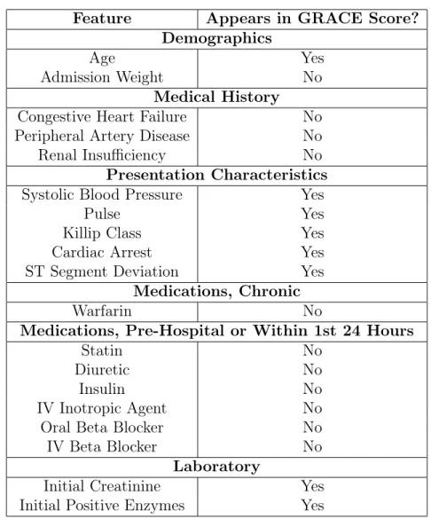
BLR identified 19 clinical features out of 198 clinical features available within the first 24 hours as being the most predictive (Table2.1). A L2 regularized model using the 19 features has an AUC on the holdout set of 0.852, which is similar to the AUC of a L2 regularized model using all 198 features (AUC 0.859, p = 0.127).
2.2.2
RLRVI Performance on the Development Set
A development set of 43,063 patients was constructed by collecting all patients who had values for all features identified by BLR. Table 2.2 shows the distribution of patient characteristics in the development set.
The RLRVI model has improved discriminatory ability relative to the GRACE score in the bootstrapped test sets, as well as the STEMI, NSTEMI, and UA subsets, as measured by the AUC (Fig. 2-2a). Similarly, HRs for all subsets show a statisti-cally significant improvement over the GRACE score (Fig. 2-2b). The RLRVI model correctly classifies more patients than GRACE in all patient subsets, as evidenced by a positive two-category NRI of 0.0337 (standard deviation over 100 bootstrapped
test sets 0.0149). Most notably, in patients who fall within the lowest 14% of risk (GRACE score ≤ 87), the RLRVI model yields significant improvements in both the discriminatory performance (Fig. 2-2c) and HR (Fig. 2-2d) relative to the GRACE score.
2.2.3
Evaluating the Relative Importance of Non-GRACE Score
Features
To determine the relative importance, over the standard GRACE score features, of each of the non-GRACE features in our model, we computed performance metrics for the RLRVI model when only the 8 GRACE score features plus one non-GRACE score feature was used as input. As the RLRVI model can accommodate 19 features as input, values for the remaining 10 features were estimated using the data imputation approach described in the methods section. Adding each of the 11 non-GRACE score features to the 8 GRACE score features yield AUCs that are improved relative to the GRACE score values (Fig. 2-3).
2.2.4
RLRVI Discriminatory Ability Using a Subset of Clinical
Features
We sought to determine how the RLRVI model performs when the number of available clinical variables changes. If there are 𝑁 < 19 features available, we could compute AUCs for the RLRVI model when only those N features are available, using data imputation to estimate the missing parameters. To determine what subsets of clinical features (if any) yield improvement when added to the established 8 GRACE score features, we considered all possible combinations of the remaining 11 features, giving 2,047 possible models.
We trained and tested each feature combination over 10 bootstrap splits of the development set. Fig. 2-4 shows the AUC averaged over the 10 bootstrap splits for each possible feature combination. For all models, the RLRVI model provides improved discriminatory ability relative to the GRACE score with p < 0.003.
Feature Appears in GRACE Score? Demographics
Age Yes
Admission Weight No
Medical History Congestive Heart Failure No Peripheral Artery Disease No Renal Insufficiency No Presentation Characteristics Systolic Blood Pressure Yes
Pulse Yes
Killip Class Yes
Cardiac Arrest Yes
ST Segment Deviation Yes Medications, Chronic
Warfarin No
Medications, Pre-Hospital or Within 1st 24 Hours
Statin No
Diuretic No
Insulin No
IV Inotropic Agent No
Oral Beta Blocker No
IV Beta Blocker No
Laboratory
Initial Creatinine Yes Initial Positive Enzymes Yes
Table 2.1: Features selected by the bootstrap lasso. GRACE = Global Registry of Acute Coronary Events; IV = intravenous.
2.2.5
RLRVI Performance on the Validation Set
A validation set, which contains patients who were not used to develop either the RLRVI model or the original GRACE risk model, was used to further assess the model’s performance. Table 2.2 shows the distribution of patient characteristics in the development and validation sets.
The RLRVI model has improved discriminatory ability relative to the GRACE score Fig. 2-5a and offers statistically significant improvement in all HRs in the vali-dation set except the UA subgroup Fig.2-5b. The two-category NRI on the validation set is 0.0191, however, the standard deviation over 100 bootstrapped test sets is high
(0.0315). In the lowest risk patients, the RLRVI model also has improved discrimi-natory ability in all patient subgroups Fig. 2-5c and offers improved HRs in all but the UA subgroup Fig.2-5d.
Development Set Validation Set
Population Size 43,063 6,363
Low-Risk (GRACE Score ≤ 87) 13,205 1,665
Mortalities 3,078 (7.15%) 719 (11.3%) Demographics Age (years) 66.1 (55.7-75.8) 68.2 (57.1–77.6) Female 32.6% 33.9% Height (cm) 170 (162–175) 169 (161–175) Admission Weight (kg) 77.0 (67.0–88.0) 77.0 (67.2–87.2) Medical History (%)
Congestive Heart Failure 10.5 11.1
Peripheral Artery Disease 9.7 9.2
Angina 51.9 45.5
Coronary Artery Bypass Graft (CABG) 12.6 11.9
Myocardial Infarction (MI) 30.3 31.0
Hypertension 62.1 61.6
Hyperlipidemia 48.3 48.1
Diabetes 25.1 26.3
Percutaneous Coronary Intervention (PCI) 17.7 17.7
Smoking 57.7 53.0
TIA/Stroke 8.3 9.1
Renal Insufficiency 7.8 8.0
Presentation Characteristics
Systolic Blood Pressure (mmHg) 140 (120–160) 140 (120–160)
Pulse (bpm) 77 (65–90) 77 (65–90)
Killip Class I 83.3% 81.6%
Killip Class II 12.0% 12.6%
Killip Class III 3.9% 4.6%
Killip Class IV 0.8% 1.3%
Cardiac Arrest 1.7% 2.3%
ST Segment Deviation 54.8% 53.1%
Medications, Chronic Use (%)
Warfarin 4.5 5.2
Medications, Pre-Hospital Acute or Within 1st 24 Hours in Hospital (%)
Oral Beta Blocker 69.8 67.1
Statin 51.0 56.6
Diuretic 25.3 28.0
Insulin 14.3 16.0
IV Beta Blocker 12.9 11.5
ACE Inhibitors 47.6 47.4
Medications, Within 1st 24 Hours in Hospital (%)
Aspirin 90.3 86.6
Laboratory
Initial Creatinine (mg/dl) 1.0 (0.9–1.3) 1.0 (0.9–1.3)
Initial Positive Enzymes 46.8% 50.7%
Table 2.2: Population characteristics in the development and validation sets. Num-bers for continuous variables are presented as the median with the interquartile range in parentheses. GRACE = Global Registry of Acute Coronary Events; CABG = coronary artery bypass grafting; MI = myocardial infarction; PCI = percutaneous coronary intervention; TIA = transient ischemic attack; IV = intravenous; ACE = angiotensin converting enzyme.
Figure 2-2: RLR Performance on the Development Set. AUCs and six-month hazard ratios in the overall (a,b) and low-risk (GRACE < 87) subset (c,d) of the development set. Error bars show one standard error of the mean. * indicates p < 0.001. Numbers above the bars indicate mean values. AUC = area under the curve; GRACE = Global Registry of Acute Coronary Events; RLRVI = ridge logistic regression with variable inputs; STEMI = ST elevation myocardial infarction; NSTEMI = non-ST elevation myocardial infarction; UA = unstable angina.
Figure 2-3: Evaluating the Relative Importance of non-GRACE Score Features. AUCs from adding one of the 11 non-GRACE score features at a time and imputing the remaining features. AUCs are averaged over 100 bootstrapped test sets. Error bars show one standard error of the mean. All models show improved performance over the GRACE score with p< 0.001. AUC = area under the curve; GRACE = Global Registry of Acute Coronary Events; RLRVI = ridge logistic regression with variable inputs; Hx = History; Peri Vasc Dis = peripheral vascular disease; IV = intravenous; CHF = congestive heart failure.
2.3
Discussion
Risk stratification models that are used in clinical practice are often constructed using regression models that take a fixed number of clinical variables as input [3–
5,8,55]. Variables that are thought to have prognostic significance are identified using a combination of expert opinion to first identify potential clinical characteristics followed by stepwise regression [62]. For example, the GRACE dataset – a registry derived from 94 hospitals across the globe – contains over 1400 clinical variables. In order to develop a risk model that could be used in clinical practice, a small subset of clinical variables (usually less than 50 features), which are typically available at presentation, was chosen based on published results from prior studies and expert clinical opinion [7,8,57]. Features in this list that had the greatest association with all-cause mortality were then selected and backward elimination was used to arrive
Figure 2-4: RLRVI Discriminatory Ability Using a Subset of Clinical Features. AUCs averaged over 10 bootstrap splits of the development set for all possible combinations of the 11 non-GRACE score features selected by BLR. The red line and numbers indicate the number of features that were known and therefore not imputed. For example, the red 6 indicates that all points in that range were generated by models that had six of the non-GRACE score features available; all possible combinations of 11 choose 6 are represented in this range. The performance of the GRACE score on the same 10 bootstrap splits is shown by the dashed line at the bottom of the plot. All feature combinations show improvement over the GRACE score with p < 0.003. AUC = area under the curve; GRACE = Global Registry of Acute Coronary Event. at a regression model that included 14 features. A simpler model, which only uses 8 features that contain the most predictive information, was then provided for clinical use [7].
As backward elimination, and, more generally stepwise regression, involves evalu-ating the performance of many models that contain different numbers of explanatory variables, the process becomes intractable when a large number of candidate variables are considered. For example, backward elimination using the 198 candidate variables we considered in this work would require training over 19,000 models to explore the different possible subsets of clinical variables. In these situations, expert knowledge forms an effective platform for limiting the number of potential variables, thereby a
Figure 2-5: RLRVI Performance on the Validation Set. AUCs and six-month hazard ratios in the overall (a,b) and low-risk (GRACE < 87) subset (c,d) of the validation set. Error bars show one standard error of the mean. * indicates p < 0.007. Numbers above the bars indicate mean values. AUC = area under the curve; GRACE = Global Registry of Acute Coronary Events; RLRVI = ridge logistic regression with variable inputs; STEMI = ST elevation myocardial infarction; NSTEMI = non-ST elevation myocardial infarction; UA = unstable angina.
making comprehensive stepwise regression computationally tractable. While expert knowledge is a powerful resource that can be leveraged to identify the most important prognostic features, relying too heavily on expert opinion limits our ability to discover previously unappreciated characteristics that have prognostic value. We therefore im-plemented a feature selection technique based on a machine learning method called BLR [59]. Unlike traditional stepwise elimination, BLR can accommodate large fea-ture sets, thereby eliminating the need to use expert knowledge to pre-prune the feature set before feature selection. In the present study, BLR identified 19 prognos-tic features from our original list of 198 by constructing only 100 models from 100 bootstrap rounds; i.e., one model for each bootstrap iteration. The fact that eight of the 19 features identified by BLR also appear in the GRACE score further
sup-ports the validity of using this automated feature selection method to generate feature sets Table 2.2. Moreover, one of these 19 features (chronic warfarin use), although available at patient presentation, was not considered in the full GRACE model that included 48 features that were identified by clinical experts, thereby demonstrating the ability of the method to discover new features with prognostic significance.
Although BLR, in general, facilitates the identification of a small set of features that can be used to build parsimonious risk stratification models, its effectiveness is limited in cases where features are highly correlated. For instance, given two important collinear features, BLR might select one in 50% of the bootstrap splits and the other in the remaining 50% of the splits. Moreover, as the method focusses on features that are consistently selected across different bootstrap splits, neither of these features would be identified as being important. While comprehensive stepwise regression avoids this problem by explicitly building models that include all possible feature combinations, it is associated with a significant computational cost when the number of potential features is large. Therefore, while BLR is not guaranteed to find all important clinical features, it does identify a subset of features that can be used to build effective risk stratification models. In this work, the model developed using only 19 features – representing less than 10% of the features available within 24 hours of presentation – has similar performance relative to the model developed using all 198 features. Models that utilize a parsimonious list of features are often easier to interpret and less likely to be over fit to a given training set. We further note that it is possible to remove correlated features from the initial feature set using a filter based on the covariance matrix. This would result in a starting feature set with independent features on which we could apply feature selection. Nonetheless, we emphasize that our goal was not to arrive at a feature set with independent features, but a model with adequate performance for the problem of interest.
![Figure 1-2: AS of increasing severity [42].](https://thumb-eu.123doks.com/thumbv2/123doknet/14726221.571838/28.918.237.676.315.468/figure-as-of-increasing-severity.webp)