Developing automated tools to analyze synaptic calcium events

Developing Automated Tools to Analyze Synaptic

Calcium Events

by

Alyssa Weiss

Submitted to the Department of Electrical Engineering and Computer

Science

in partial fulfillment of the requirements for the degree of

Master of Engineering in Electrical Engineering and Computer Science

at the

MASSACHUSETTS INSTITUTE OF TECHNOLOGY

May 2020

c

○ Massachusetts Institute of Technology 2020. All rights reserved.

Author . . . .

Department of Electrical Engineering and Computer Science

May 12, 2020

Certified by . . . .

Troy J. Littleton

Professor

Thesis Supervisor

Accepted by . . . .

Katrina LaCurts

Chair, Master of Engineering Thesis Committee

Developing Automated Tools to Analyze Synaptic Calcium

Events

by

Alyssa Weiss

Submitted to the Department of Electrical Engineering and Computer Science on May 12, 2020, in partial fulfillment of the

requirements for the degree of

Master of Engineering in Electrical Engineering and Computer Science

Abstract

Synapses are the fundamental building blocks of the nervous system. Neuroscien-tists use electrophysiological approaches to measure synaptic release, which lack spa-tial resolution to measure synaptic transmission at the resolution of single synapses. One challenge in accurate measurements is the lack of reliable quantitative tools to detect synaptic signals from individual synapses. Moreover, the small size of synapses makes it tedious to measure synaptic transmission and analyze it manually. To over-come this problems, in this thesis, a range of tools to analyze calcium florescent images of synaptic regions were implemented and developed in order to create a pipeline for gathering synaptic release information from calcium imaging data. Using this analysis pipeline, we quantified synaptic signals, mapped the probability of release and applied machine learning tools to classify synapses as high and low probability synapses. The final result of this thesis aims to demonstrate that it is possible to create a set of tools that can automate the process of calculating synapse release information at a level that drastically improves upon the efficiency of manual work and that has, ideally, near human accuracy.

Thesis Supervisor: Troy J. Littleton Title: Professor

Acknowledgments

The completion of this thesis would not have been possible without the hard work and time from multiple people in the Littleton Lab. I would like to thank Dr. Suresh Kumar Jetti for his guidance throughout this process. He introduced me to the project and provided support throughout the process, and I appreciate all of the help he provided. I would also like to thank Professor Littleton for supporting this project and providing guidance and support on the writing of this thesis. I would also like to acknowledge Grace Tang and Dr. Sourish Chakravarty (postdoc fellow in the Brown lab) for their technical contributions to this project. Their work with ROI identification and motion correction was crucial in helping to develop an efficient pipeline for analysis. I would also like to thank Yulia Akbergenova for her help throughout the process in discussing what features of successful annotation would be considered important. I truly appreciate all of the help from everyone in the Littleton Lab.

Contents

1 Introduction 11

1.1 Background . . . 11

1.2 Thesis Goals . . . 12

1.3 Related Works . . . 13

1.3.1 Calcium Imaging for Neurons . . . 13

1.3.2 Previous Work at Littleton Lab . . . 15

1.3.3 Work Preparation for this Project . . . 16

2 Imagine Analysis Pipeline 19 2.1 Pipeline Overview . . . 19 2.2 Motion Correction . . . 21 2.3 ROI Detection . . . 22 2.3.1 Background . . . 22 2.3.2 Application in Code . . . 25 2.4 Florescence Tracing . . . 26 2.5 P𝑟 Mapping . . . 27 2.5.1 Overview . . . 27 2.5.2 Challenges . . . 28 2.5.3 Algorithm Design . . . 29 2.5.4 Pipeline Results . . . 33 2.6 Code Pipeline . . . 34

3 High and Low Release Probability Calculations 35 3.1 Overview . . . 35 3.2 CNN Approach . . . 35 3.3 K-means Approach . . . 37 3.3.1 Description . . . 37 3.3.2 Results . . . 39 4 Future Work 43 4.1 Overview . . . 43 4.2 Pipeline Analysis . . . 43

4.3 High and Low Release Probability Analysis . . . 44

5 Conclusion 47

List of Figures

1-1 Organization of the Drosophila Synapse . . . 12

1-2 Neuron ROI Labeling . . . 14

1-3 Synapse ROI Detection and Labeling . . . 17

2-1 Analysis Pipeline . . . 20

2-2 ROI Labeling . . . 25

2-3 Florescence Tracing Example 1 . . . 26

2-4 Florescence Tracing Example 2 . . . 27

2-5 Binary Mask Generation Matlab Code . . . 30

2-6 Flash Assignment Based on DF/F . . . 32

2-7 P𝑟 Map Results . . . 33

2-8 Code Pipeline . . . 34

3-1 Release Classification Map Example One . . . 40

A-1 Additional P𝑟 Map Additional Example One . . . 50

A-2 Additional P𝑟 Map Additional Example Two . . . 51

A-3 Additional P𝑟 Map Additional Example Three . . . 52

Chapter 1

Introduction

1.1

Background

Synapses, the fundamental building blocks of the nervous system, are specialized devices of neuron-to-neuron information transfer [9]. At the synapse, the electro-chemical signals from the presynaptic neuron exit the neuron’s axon terminal, and are passed to the dendrite of the postsynaptic neuron. Being able to analyze information about these synaptic communications has important effects in understanding brain function, and having accurate information on timing and intensity of these commu-nications would allow for significant advances in topics such as understanding certain neurological disorders or analyzing the effect of certain medications. The traditional and most common method used to study synaptic communication in neural circuits is electrophysiology [8]. However, while electrophysiology is effective for quantifying how an ensemble of individual synapses participate in neuron to neuron communi-cation, it does not allow for a strong analysis of the communication that occurs at individual synapses. To resolve this problem, the Littleton lab has developed ge-netic and imaging technology to address this fundamental challenge in neuroscience research. Building on top of the work that has been done so far, a problem that remains is that there are no standard analytical tools to measure how individual synapses communicate in a reliable and robust manner. To address this problem, in this thesis, I aim to develop quantitative tools to analyze synaptic calcium imaging

data and release probabilities of synapses in a manner that is as accurate as human manual analysis and significantly more efficient, where a significant improvement in efficiency represents a significant amount of time saved as compared to work done manually.

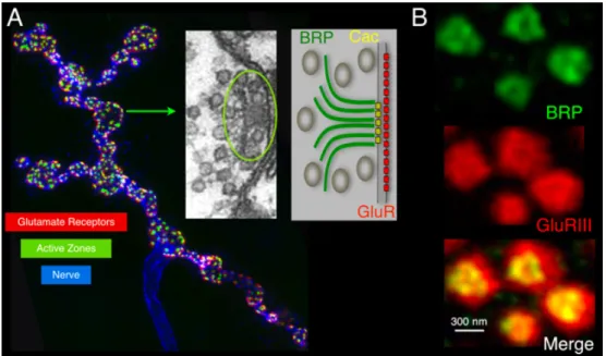
Figure 1-1: Organization of the Drosophila Synapse: immunolabeling of the axon (anti-HRP, blue), active zones (anti-BRP, green) and postsynaptic compartment (anti-GluRs, red). Electron micrograph of an active zone (AZ) with the electron dense T-bar (circled) and associated synaptic vesicles. Each dot represents a synap-tic vesicle. A model of the AZ with BRP (which forms a T-bar filamentous structure), Cac (N-type Ca2+ channel) and postsynaptic GluRs is on the right. 1B. Nanoscale organization of synapse: STED imaging of AZs (green, anti-BRP) and their apposed postsynaptic densities (PSDs; red, anti-GluRIII).

1.2

Thesis Goals

Aim 1. Create a pipeline for detecting the location of synapses, extracting calcium signals and mapping release probability: The data used in this thesis was collected by Drs. Jetti and Akbergenova from different types of synapses that differ in their release probability and response kinetics. The first aim of the work in this thesis is to create

a pipeline to analyze release probability of individual synapses. This pipeline, as will be described in detail, includes applications of various tools to handle challenges such as motion correction, Active Zone (AZ) releases that cover multiple AZs, and dimming of calcium signals over time. The pipeline is designed so that, as input, it can take in videos of the calcium florescence intensity of a neuron over time, and output a mapping of all synapses in the neuron to their release probabilities. Additional information, such as the DF/F traces of all synapses over time, is also generated from the output of this pipeline.

Aim 2. Determine the classification of the release probability of individual synapses. The goal here is to provide tools be able to classify synapses as high or low release probability with machine learning approaches such as K-means clustering.

1.3

Related Works

1.3.1

Calcium Imaging for Neurons

In the field of analyzing calcium florescent images, there have been multiple ap-proaches to developing tools for automatic analysis of calcium imaging data for the neurons [18]. However, such sophisticated tools are still lacking to analyze synaptic calcium signals at the level of individual AZs. One such example of a similar project applied at a neuron level is the CalmAn project, which is an open source tool for calcium imaging data analysis [7]. CaImAn provides the ability to analyze neuron images with calcium florescence and provides analysis on different types of models that can be used to extract information from calcium images. CaImAn is able to use Convolutional Neural Nets (CNNs) to perform neuron location detection on calcium florescent images at near human accuracy. CNNs are a machine learning tool that are often recommended to be used for image analysis, as they can use training data to learn to recognize image feature that are of significance. The goals of the project are different from this thesis, as CaImAn is focused on the detection of calcium signals from neurons rather than from the synapse, which is harder to achieve. There are

currently no such tools that are able to apply similar ideas from the CaImAn project to actual synapse analysis, as the small size of synapses and the variety of shapes of synapses makes them more challenging to analyze. Although the applications of the CaImAn are different from the aim of this thesis, having an understanding of this work provided insight into what types of tools may be most successful at working with calcium florescent images.

Figure 1-2: Analysis comparing neuron Region of Interest (ROI) labeling with synapse ROI labeling. (a) shows an image of multiple neurons with the ROIs labeled (the neurons are outlined in white), and (b) shows an image with multiple synapses with ROIs outlined. This highlights the differences in size, shape, and closeness of ROIs on the neuron level and on the synapse level.

The differences between the two images in Figure 1-2 highlight some of the key differences between analyzing calcium images of neurons compared to analyzing cal-cium images of synapses. At the neuron level, neurons are much more likely to be clearly circular and spaced apart. At the synaptic level, however, there is much larger variation in the shape and size of individual ROIs, even within a single image. This variation in shape and size makes finding an efficient and consistent way for identi-fying ROIs much more difficult. In addition, another added difficulty at the synaptic level is that the synapses tend to be much closer together. This creates an

addi-tional level of complication for locating ROIs, as well as for other steps of analysis. For example, the staining from the calcium florescence when a synapse releases can spread over an area outside of an individual synapse. This means that analyzing if an individual ROI has released is not as simple as analyzing the stain of the ROI across time, because a big problem is that the staining can appear on one ROI even if the actual origin is from a different ROI. This potential contamination requires careful working in making sure to properly assign flashes to the correct ROI. The figure and these challenges described aim to highlight the difficulties in transferring work done on analyzing calcium florescent neuron images to calcium florescent synapse images, and highlight why it is important to develop tools specifically for this purpose.

1.3.2

Previous Work at Littleton Lab

The Littleton Lab at MIT has been generating the types of images that, through this project, we hope to be able to provide further analysis to. The method for col-lecting this data is detailed in multiple papers published by the lab [12], [1]. Calcium imaging data was collected from the 3𝑟𝑑 instar larvae of Drosophila. Flies of both sexes are used, and all flies are cultured on standard medium kept at 25∘ C. To be able to track when synapses fire, a fluorescent marker is needed, so for the purposes of this work Ca2+ sensor GCaMP6m was attached to the neuronal plasma membranes of the flies. To capture images, a Zeiss Axio Imager two spinning disc confocal head was used in combination with a ImagEM X2 EM-CCD camera. Images were collected continuously for varying time lengths, generally up to 10 minutes. When images were collected, if there were slight movements that effected the location of synapses in the frame of view, the images were corrected manually. If movement was too drastic that this correction was not possible, the data files are not considered for further analysis and were discarded.

Prior to this project, the Littleton Lab was able to collect important results from the analysis of these calcium images. For example, calcium imaging was collected for the same AZs for both spontaneous and evoked release to determine if these were correlated [12]. From the work, the conclusion was able to be made that these

two types of release are regulated independently and that there are two separate channels for regulating evoked and spontaneous synaptic release. Another project that required similar analysis was the study of how the molecular composition of synapses in Drosophila is correlated with their release probabilities. This work was able to provide analysis on certain correlations, such as demonstrating that release probability is associated with factors such as AZ age and the prevalence of glutamate receptors.

1.3.3

Work Preparation for this Project

Foundational analysis for identifying synapses in these types of image described above began through the Littleton Lab. One important piece of work that was started was the creation of a Matlab pipeline for allowing an individual to take a scan in the form of either a single still frame or a video of frames over time, and manually mark ROIs, in this case synapses. The results from this manual annotation is then saved in a format that saves the corner points of the polygons of each located synapse. This code is important because it provides a standard way of marking data so that it is repeatable and can be easily used on new data and by different researchers. It is also important to note that there can be discrepancies among data that are manually labeled by different individuals. One potential approach for handling discrepancies is to have multiple researches separately annotate all data, and have a discussion on any mismatches between annotations so an official ground truth of correctly annotated data can be created [7]. To address this concern during the duration of his project, we worked to develop a standard for correctly annotating images, and worked with other researchers (Sourish Charavarthy, postdoc in the Brown lab) to develop “gold standard” images reflecting correctly annotated versions of files.

Another piece of work that began before the start of this thesis were initial at-tempts at code to automatically identify the location of synapses given the results of the data. This work, done in Matlab, takes in a tif file and creates outlines for the synapses, that it is able to recognize. It does this detection by having a baseline threshold for what the florescence should be, and marking ROIs as areas where the

florescence is significantly higher than the baseline threshold. An example of the differences between the current automatic recognition of synapses versus a manually labeled version of the same image is demonstrated in Figure 1-3, where demonstrates that there is not full accuracy in this original implementation of automatically iden-tifying synapses.

Figure 1-3: (a) Representative image showing data file generated from the method described above. In this image, each red dot represents a synapse (post synaptic com-partment labelling) and green area represents membrane tagged version of genetically encoded calcium indicator GCaMP (b) shows the automatic detection of synapse lo-cations based on the original version of code that had been worked on prior to the start of this thesis, and (c) shows an example of synapses being marked manually. The number of marked synapses in (c) that are missed in (b) demonstrate the caveat of the automatic detection and emphasize the importance of having correct labels.

Chapter 2

Imagine Analysis Pipeline

2.1

Pipeline Overview

In order to analyze calcium imaging data, there have been a few standardized pipelines that have been developed. For the purposes of this project, a similar pipeline was followed to what is discussed in the Science Direct publication “Analysis pipelines for calcium imaging data” [19]. As outlined in this article, the pipeline developed involves first applying a motion correction algorithm to the movie file, then locating the ROIs in the movie file, next extracting the DF/F traces from all of the identified ROIs, and finally using those DF/F traces to calculate release probabilities at each ROI. An example of the full pipeline applied to a single movie input can be seen in Figure 2-1. The steps work together to make a pipeline that is an efficient and scalable approach to analyzing these calcium florescent movies.

(a)

(b)

(c)

Motion Correction Alignment

Labeled ROIs

DF/F Traces

(d)

(e)

Pr Mappings

Figure 2-1 shows the full pipeline of video processing starting with the movie and resulting in a Pr map of synapses. (a) outlines the steps in the pipeline. (b) demon-strates how the motion correction works, showing the red channel resulting by av-eraging across frames and the red channel of a later frame. The regions of these channels that have higher pixel color values are matched so that later frames can be shift adjusted to align with the first frame. (c) shows the result of ROI annotation, with each ROI outlined with a white line. (d) shows the resulting DF/F traces, with a trace for each of the synapses outlined in (c). Finally, (e) shows the final resulting Pr maps, which map each ROI to its release probability. The left image labels each ROI with its release probability, and the right image is without labels to generate a clearer image.

2.2

Motion Correction

The first step in the pipeline is motion correction. The need for motion correction arises because, as multiple images are being taken over the course of a calcium image scan, any slight shifts in the frames can have a drastic effect on tracking the florescence of an ROI. The DF/F calculations are very dependent on the colorings in the exact pixels that represent a given ROI, so a shift even of a few pixels can drastically effect the results. The problem becomes even more amplified in these applications at the synaptic level. Considering the small size of the synapses, shifts that may seem insignificant can actually end up shifting the frame enough that the original outline of an ROI no longer overlaps with the actual location of the ROI in a new frame. With these concerns in mind, it is clear that finding an appropriate way to handle motion correction was an important issue to address.

For the purposes of this project, we were able to use the Non-Rigid Motion Correc-tion (NoRMCorre) algorithm, a Maltab implemented algorithm for frame by frame motion correction in calcium imaging data [20]. The choice of this algorithm and implementation of this algorithm in the applications for this purpose was completed in collaboration with Grace Tang. There are ranges of motion correction algorithms

for calcium imaging that have been explored, as having videos with correct motion correction is important for the accuracy of results, and these algorithms can range drastically in their runtime and scalability [13], and for the purposes of this applica-tion NoRMCorre was considered the most appropriate to match the needs and scale of data. This motion correction algorithm works by first calculating a reference tem-plate, that is calculated as the average across all of the frames. This is then used as reference for how to provide motion correction for all of the individual frames. For each frame, a displacement vector is calculated representing the shift between the frame and the reference template. Once all shifts have been calculated, the correct pixel shifts can be applied to each frame, and the output represents each frame motion corrected to match the reference.

For the purposes of this application, motion correction is applied to individual color channels. When calculating the reference template and the displacement vectors for each frame, the red channel is used. This is because the synapses are marked genetically using a postsynaptic markers (glutamate receptor subunit-A) in red, so by looking only at the red channel we except to see only the synapses themselves, and the synapses can be aligned across frames. If the green channel would be considered, this would also include the coloring as various synapses fire, which we would expect to be variable across frames. Since we want to align based on elements that are consistent across the frames, we only use the red channel. Once all of the distance vectors are calculated, the shifts can be applied to each individual color channel. Because only red and green channels are needed for later analysis, motion corrected versions of the frames are only computed for those two channels.

2.3

ROI Detection

2.3.1

Background

As described previously, ROI detection in synaptic images presents a range of challenges. As compared to neuron ROI detection, synapses are much more variable

in both size and shape, and can be spaced very close to each other, making it difficult to distinguish boundaries. For the purpose of this project, the focus of ROI detection was on a Matlab procedure that allows for efficient human labeling of ROIs. After much discussion and consideration, this was deemed the most appropriate approach for this project for a few reasons. In order to make sure the pipeline is accurate, having correct ROI labels is extremely important. It is important to not miss any ROIs in the ROI detection step, or else they will not be considered later, and any flashes from that ROI could be misattributed. In addition, there are similar concerns with mislabeling ROIs and not separating two ROIs that are located in close proximity.

Once concern with having human input is that this leaves room for human error. To address this problem, for the purposes of this project we had multiple people look at every image that was annotated. If there were any ROIs that one individual labeled and someone else did not, this allowed for an analysis of the differences and, a final “gold standard” correct labeling could be completed.

Another concern with this approach is that it does detract some from the efficiency of the pipeline, as it requires manual input to label the ROIs. Because this was a concern, some approaches that would not require the same level of human interaction were considered. One such approach was to consider the red channel of the image and analyze the intensity of the red channel for each pixel in the image. Then, a baseline intensity threshold was set. Next, any pixel that was above the baseline threshold intensity was considered to be part of an ROI. Finally, all clusters of pixels that were connected and above the baseline threshold were considered a single ROI. This approach was effective at correctly noting which pixels were parts of ROIs, but was very sensitive to the threshold set, and this made it very difficult to apply correctly. If the threshold was set too low, then some pixels that were near ROIs but not inside an ROI would still be above the threshold. This was particularly problematic for ROIs that were close to each other, as the pixels in between them could then still be considered part of an ROI, and when grouping all touching pixels, this would cause neighboring ROIs to be counted as a single ROI. However, if the threshold was set too high, other problems could arise, such as ROIs could be missed if the pixels in

that ROI were not above the threshold. Because intensities can differ across different images, and even across ROIs in a single image, finding any baseline intensity that would work for this problem proved extremely difficult, and this approach was not considered to be the best option.

After identifying the issues in the previous approach, an adaptation of the above approach was considered. This approach had a similar start, by setting a threshold and analyzing the red channel to identify pixels with an intensity value above that of the threshold. For the next step, instead of simply separating ROIs based on the connected pixels above the threshold, a watershed transformation was applied. In order for the watershed transformation to be applied, the image is first redefined as a 2d array of 0s and 1s, where 0 represents pixels below the threshold values, and 1 represents pixels above the threshold. Next, for each pixel, the bwdist is calculated for each pixel. Bwdist is a measure of how far each pixel is from a 0 valued pixel. The bwdist value will be 0 for all pixels below the threshold, and for all pixels above the threshold will represent the closest distance to a pixel that is below the threshold. Finally, the watershed transformation is applied. This transformation separates pixel clusters into clusters that appear to be coming from the same source by analyzing the bwdist values, and calculating if the distances appear consistent with one object or with two objects that are touching. The benefit of this approach over the previous approach is that it is able to separate out two neighboring ROIs. However, after testing against multiple images, it was evident that this method created the issue of sometimes splitting a single ROI into multiple ROIs. Again, finding a threshold value that could produce consistent and accurate results was challenging.

With these methods considered, another approach that could allow for a more automated ROI detection would be to use a CNN to automatically detect ROIs. Previous work that has been done with calcium imaging on the neuron level suggests that CNNs have the potential to be successful at ROI detection [10]. While this approach was discussed, it was not considered to be appropriate for this version of the project, as the number of data samples required for sufficient training were not available. In order to train a CNN, large number of labeled and annotated images

would be required, in order for the model to be able to confirm the validity of the output. By creating an efficient process for manually labeling ROIs, we aim to not only create a labeling scheme that can be used for this process, but to also create an increase in the number of accurately labeled data files, that could be used in future work if the decision to implement a CNN for this purpose is further explored.

2.3.2

Application in Code

To start annotation of ROIs, a file that is either a .tif or .mov is taken as input into the annotation code. Then, the user is able to draw directly onto the image, and click to label the ROIs. An example of the labeling in steps is outlined in figure 2-2. The codes for this section were developed by Sourish Chackravarty, a postdoc in the Brown lab.

Figure 2-2: Shows an image updating as the user continues to outline ROIs. Moving left to right in the image, there are an increasing number of labeled ROIs.

After the user exits the images labeling session, the results are saved in a .mat file. For each ROI, the coordinates of all of the corners (shown as stars in the images), which represent where the user clicked, are saved in this .mat file. Later, whenever the locations of the ROIs are required, they can be accessed by calling load(filename). For purposes of this pipeline, a function is called converts from the list of the corners of each ROI to a layers of masks. In this layer of masks, there is one for each ROI. Each ROI mask is the size of the image, and has the value 1 for pixels labeled portion

of the ROI, and 0 otherwise. Being able to generate these masks are useful for next steps in the pipeline of florescence tracing and Pr mapping, as they allow for quick analysis of the intensities of different ROIs across different frames.

2.4

Florescence Tracing

Once the videos are motion corrected and ROI detection is complete, the next step in the pipeline involves florescence tracing for each ROI. This step is useful on its own because having these traces can prove useful for certain analysis. In addition, being able to study and understand trends in the fluorescent traces of synapses was important for assigning release flashes to the correct ROI, and can be used to compare against the final resulting Pr maps. While analyzing florescent traces, both overall florescent intensity and DF/F traces were generated and analyzed.

To generate florescent traces for each ROI, the first step involves calculating the green florescence intensity for each ROI at each frame. This is done by stepping through each frame, and going over each ROI in the frame, and taking the mean of the values of the pixel in the green channel of the image for all pixels that are located within the boundaries of the ROI. This calculation is enough to be able to generate florescent traces for each ROI. To be able to generate DF/F traces, the median green intensity for each ROI can be calculated by taking the median of the green intensity across all frames.

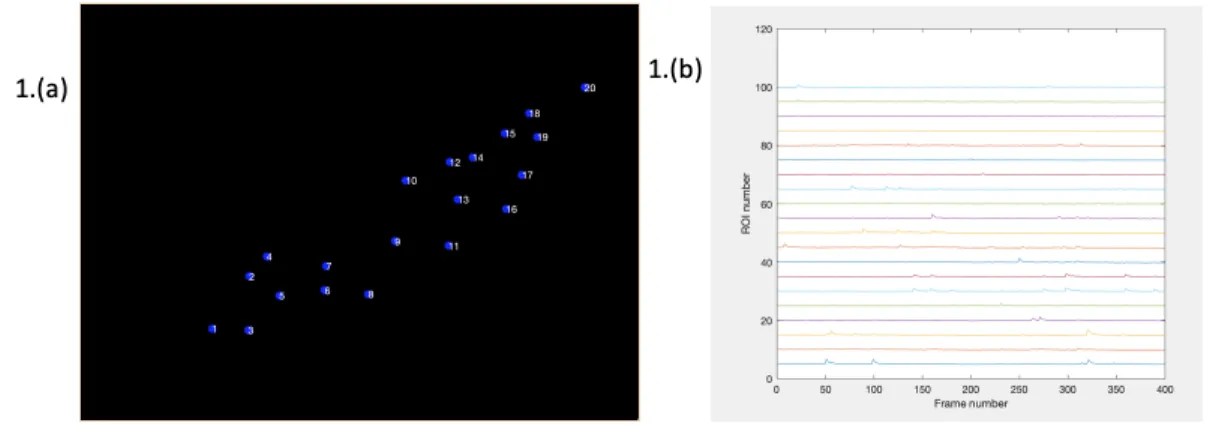
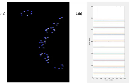
Figure 2-4: Second Example of Florescence Tracing: this image and image 2-3 show the types of output that are able to be generated with the florescence tracing portion of the pipeline. In both images, (a) shows a plot with all of the synapses labeled and numbers. The numbers on these plots correspond with the ROI number for parts (b) Part (b) if each image shows the DF/F trace for each ROI. The trace for ROI is plotted as a separate line, and is plotted across the whole movie, as represented by increasing frame number.

2.5

P

Mapping

2.5.1

Overview

Creating a method for accurately calculating the release probabilities of each synapse proved to be a challenging component of this pipeline. In order to calculate the release count (number of times a synapse fires for a spontaneous video) or release probability (percentage of stimuli for which a synapse fires for an evoked video), the total number of times that each synapse fires needs to be counted. This requires iter-ating through all frames in the video and assigning any flashes that appear in them

to the appropriate synapse.

2.5.2

Challenges

Although there have been other attempts to solve this problem of assigning flashes correctly to a synapse, there are multiple challenges that presented themselves in this work. There were a few challenges that needed to be taken into consideration when developing this approach, and the difficulties these created needed to be addressed carefully in the code. These challenges are summarized below.

Dimming Over Time

One problem with the way calcium florescent imaging works is that, over time as the imaging is collected for the movie, the intensity of the florescent stain may fade. This is problematic because it means that a constant threshold cannot be set to determine what represents a flash, or a synapse firing. While the start of the movie may see all flashes of a certain green channel intensity, it is possible that the color can be only half of that intensity by the end of the video. Because of this, the threshold for determining what constitutes a flash needs to be able to adjust to various intensities across one video.

Variable Flash Lengths

A second challenge that had to be considered is that some the flashes may last a variable number of frames. While some flashes may only be visible in one or two frames, some may be visible in up to four or five frames. Because the same flash may be visible in more than one frame, each frame cannot be considered independently because that could count one single synapse firing as multiple, if it appeared on more than one frame. Because the number of frames a flash appears on is variable, there can also not be a set number if frames to ignore post a flash, because there is no consistent number of frames to skip.

Overlapping Flashes

Another problem that is tied into the fact that some synapses are located so close together is that sometimes a single flash can overlap with multiple ROIs. This means that, just because there is a greater green florescent intensity in an ROI at a specific

point, we cannot attribute the flash to that ROI, or else we could end up attributing the same flash to multiple ROIs, which leads to over counting of the number of synapses that fired. It is very important to only assign a flash to a single ROI, so this had to be designed around carefully.

Handling Spontaneous and Evoked Releases

One final challenge that needed to be addressed in this algorithm was that it needed to be able to analyze both spontaneous and evoked synaptic releases. For videos with evoked releases, many flashes were likely to start at the same time in response to a stimulus, whereas in spontaneous videos the flashes can be much more randomly timed. It was important to make sure that our analysis was able to provide accurate results for both types of input.

2.5.3

Algorithm Design

After understanding the challenges to this problem and the issues with current approaches to the solution, we were able to design an algorithm that is efficient and addresses the challenges described above. The code for this process was developed in collaboration with Grace Tang. The steps of the algorithm are outlined below.

First, we need a baseline green intensity channel for comparisons. To do this, the minimum green intensity pixel value for each pixel is calculated, and this is used as a reference point. Next, each frame needs to be analyzed, starting at the first frame and working through the last one. For each frame, the first step is to create a binary mask highlighting any green flashes. The code for this can be seen in Figure 2-5. The inputs to this function are a frame, which is the green channel for the frame currently being analyzed, a baseline, which is baseline green image as described above, and a minimum area. The minimum area is set so that only patches of pixels that are of significant enough size will be considered. For example, we do not want to consider a single pixel that is above the baseline intensity if none of its neighbors are, because this is represents an insignificant small change in the image that could be due to various reasons, and not an actual flash. The value of minimum area is not set as a constant because this would require a single constant minimum area to be

used for different videos, and as synaptic sizes are so different across images, this is not practical. It is instead left as a variable, and the value that is passed in is the minimum ROI size, so that only increases in intensity that are at least the size of an ROI are considered.

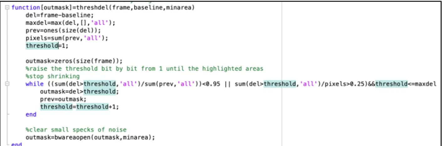
Figure 2-5: Matlab code for generating binary mask of flashes

This code works by first calculating the difference over the entire image of the current frame and the baseline green intensity values (del), and then calculating the max of these difference (maxdel). Next, prev, which is the size of the image, is set to all ones, and the total number of pixels is calculated. The threshold is initialized to one. Next the threshold is increased one by one. The output mask at each new threshold is then set to a 0 for pixel values where the difference is less than the threshold, and 1 otherwise. This continues happening as long as increasing the threshold leads to at least a five percent decrease in the number of pixels that have a difference above the threshold, or more than a quarter of the pixels are above the difference, and as long as the threshold is less than the max difference. Finally, once the final threshold value is determined, any collection of 1 pixels that is smaller than the minimum area are cleared. The resulting output mask, therefore, is 1 to represent a pixel that is considered florescent enough to be part of a flash, and 0 otherwise.

This approach to calculating what pixels in the frame are considered part of a flash was developed to address the challenge of fading calcium intensities over time. This approach avoids every having to set a fixed value to represent a threshold for what

intensity is needed to be considered as part of a flash. In addition, by measuring the threshold based on the difference in intensities at each individual pixel, this avoids problems that may occur from different base intensities that may differ across the image if, for example, there is some very dim green in the base in part of the image but not the rest.

Once the output mask is calculated, if there are any flashes (any of the pixels are labeled 1 in the output mask), this frame is analyzed. If not, the next frame is considered. Once a frame is identified as having a flash, the flash or flashes in the frame need to be assigned to the correct ROI(s). Each flash, which is identified as a cluster of 1s in the output mask that is separate from other clusters, is considered separately for analysis, as they need to be assigned to different ROIs. The next challenge that needs to be addressed is the variable flash length. In order to handle this, an end frame for the flashes needs to be found. For this to happen, the output mask is calculated for the next frame. As long as there is any flash that continues from the current frame to the next frame, the end frame is increased, until the final end frame represents the first frame where no flash continues on. To calculate if a flash is continued from one frame to the next, an element wise multiplication of the output masks for two frames is computed. If there are any pixels that are elements of a flash in both frames, then the flash has continued on into the second frame. Note that the end frame represents the end of any flashes that have started since the start frame, but that this end frame may not be the end frame for any given individual flash.

Now that an end frame has been calculated, each flash that appears between the start frame and the end frame must be analyzed. For each flash, the last frame at which that flash has a significant overlap with any of the ROIs is calculated. This is done by performing an element wise multiplication between the pixels representing the flash at a given frame with a map that has 1 for pixels in an ROI and 0 otherwise. As long as there is some overlap between the flash and an ROI, the frame is increased. Once this last frame is calculated, version of the flash that appears in this frame can be used for analysis. Now, the next step is to assign the flash to a single ROI. The

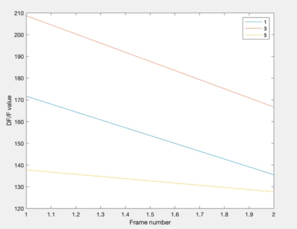
first step is finding what ROIs this flash overlaps with. If the flash overlaps with only one ROI, then the flash can be assigned to this ROI. However, if the flash overlaps with multiple ROIs, this approach will not work. In order to assign the flash to a single ROI, DF/F values where used. For all of the frames in which the flash appears, and for all of the ROIs that overlap with the flash, the DF/F values for those ROIs are computed. Then, an area under the curve approach is used, to sum all of the DF/F values over the time of the flash and calculate which ROI has the highest DF/F value. The flash is then attributed to this ROI. An example of this can be seen in figure 2-6. In that example, the ROI number had the highest DF/F values over the course of the frames in which the flash appears, so the flash is attributed to that ROI.

Figure 2-6: Shows an example of a DF/F plot over the frames for three different ROIs that a single flash overlaps with. Based on this plot, the flash would be assigned to ROI 3, as th area under the curve for ROI 3 is greater than the other two ROIs

2.5.4

Pipeline Results

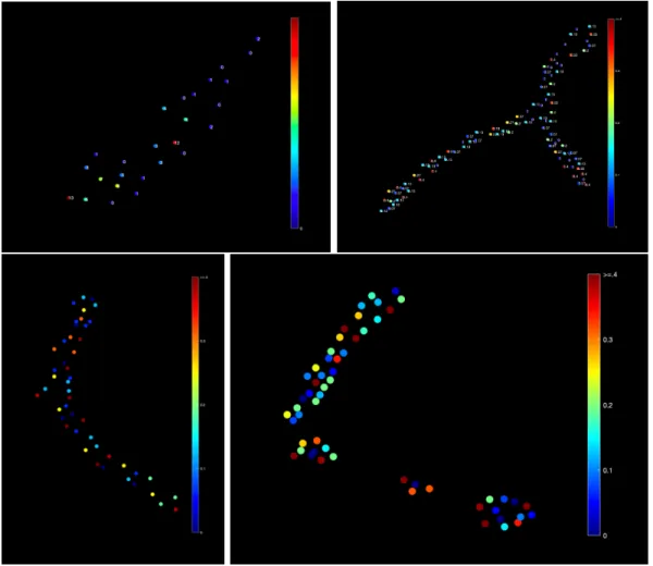
By successfully implementing the pipeline outlined above, the output is able to generate Pr mapping with release counts for spontaneous events and release proba-bilities for evoked events. Examples can be seen in image 2-7. This pipeline can be applied to a range of mov files to generate similar outputs.

Figure 2-7: Four examples of release maps that are successfully generated through this pipeline. The top left image is for spontaneous events and the release counts are shown. The other images are for evoked events and the release probability is used for the map. The top right image is labeled with release probability and the bottom three are unlabeled for a clearer image. Further examples can be seen in Appendix A.

2.6

Code Pipeline

To provide a full understanding of the codes mentioned in this section and the order of how the pipeline is run, Figure 2-8 outlines this process.

Figure 2-8: This graphic outlines the code pipeline and highlights the most important code files and what order they are called in. The first file run is the annotation file. This saves a .mat file with the labeled ROIs. Once this file is saved, the flash counter file can be run. The majority of code for this pipeline is based in this file. This file also calls upon the motion correction file (motionCorrect.m), the file for converting from the labeled .mat file to masks of ROIs (vertices2filled.m), and the thresdel file (threshdel.m), as well as a few other files that are used for analysis.

Chapter 3

High and Low Release Probability

Calculations

3.1

Overview

The probability of synaptic release varies from synapse to synapse. Some synapses release with higher probability (high ‘p’), some with low probability (low ‘p’) and some synapses remain salient. To quantify such heterogeneity in P𝑟, it is crucial to calculate

high and low ‘P’ synapses. This can be useful for making connections between certain properties of synapses and their release probability. For example, it is useful to be able to analyze if certain molecular factors are associated with a synapse being high release [1]. There are a range of features that could potentially be correlated with release probability, such as molecular composition, shape of the synapse, size of the synapse or location of the synapse within the neuron.

3.2

CNN Approach

An approach that has potential for taking advantage of the associations between synapse properties and their release probabilities is to create model that can learn to predict the release probabilities of synapses. In order to convert from information about a synapse to their release probabilities, a promising approach would be to use

a CNN. In a CNN, there is an input layer (which takes in the data), several hidden layers, and finally an output layer (which outputs a result). There are multiple nodes in each layer. At a given node, it takes the dot product of the results of the previous layer with a vector of weights that is unique to each layer. Then, an activation function is performed on this value, and the result of this function is considered the output of the node. For the purposes of this analysis, the output would be a classification of the synapse as a zero release, low release, or high release probability synapse.

One challenge with the CNN approach is that, in order for the CNN to be able to accurately predict release probability, it requires a sufficient amount of training data. This training data needs to have both the input in the format that would be put into the model when to get a probability, and the true release probability of the synapse. CNNs require a large number of data samples to be able to predict release probability of new input because they need to be trained on enough data to learn patterns in what features of the CNN may be associated with or indicative of the release probability of the synapse.

Because of the large number of training data samples that are required for a CNN to produce accurate results, the potential of this to model to be successful is limited to use on input types for which there is a sufficient amount of information available. There is evidence in prior research of associations between molecular composition of synapses and their release probabilities, so if this data was available in large enough quantities, using this CNN approach appears promising for learning associations be-tween synapse molecular composition. With the data that was available for this project, the CNN approach for the scope of this project instead aimed to classify synapses as high or low release probability based on images of the synapses.

In an effort to use a CNN model to classify synapses as high or low release prob-ability, a CNN model was trained on input data with synapse information and a classification of the synapse as high or low release probability. The information for the synapse was taken in as an image of each synapse, where the full image was a full image size, and all non-synapse pixels were set to 0. Then, for all synapse pixels the synapse value was set to the pixel value of the synapse in the image. After the model

was trained on these inputs, it aimed to be able to take as input synapse images of previously unseen synapses, and classify the synapse as either high or low release probability.

Based on the data that was available for this project, the CNN model was not able to produce results that were statistically significant. One potential reason for this is that the type of information that was being provided (visual information on the synapse) is not enough to predict anything about the release probability of the synapse. Another reason could be that more training data would be required to achieve accurate results. To address these concerns, there are multiple levels of future work and exploration that could be done on this topic. One suggestion would be to use the same model and attempt rerunning it when there is a increase in the amount of training data available. This would address the case in which the visual information is significantly correlated with the release probability, and the model was not able to produce accurate results because it did not have enough training data. If, in fact, visual information is not enough to predict release probability of synapses, this approach could still be used, but with different input data, perhaps molecular composition of information or other similar information.

3.3

K-means Approach

3.3.1

Description

After completing the analysis above, the shift in focus of this portion of the project shifted to finding an algorithm to classify the synapses in movies as high or low release probability. The goal in this analysis was to be able to take a video and calculate release counts/probabilities from the video, and then use those values to split the synapses into high, salient, low, or zero release probabilities. The challenge in this problem comes from the fact that having set release probabilities to count as high or low release may not be consistent across videos or types of neurons. For example, in one type of cell, if the highest release probability is .2, we would want to consider

something with a .2 release probability to be high release. However, if the type of cell had an average release probability of .2, then we would want to consider a synapse with a .2 release probability to be considered salient. Therefore, the approach to this problem needed to be adjust to different input types. In an effort to minimize human input and automate the process, using a machine learning tool was deemed the most appropriate approach. This allows for the data to be analyzed automatically and prevents the user from having to make any decisions on what thresholds should be set for high and low release probabilities.

To approach this classification problem, a K-means clustering approach was used. K-means clustering is an unsupervised machine learning tool, meaning that it does not need labeled input data, like the CNN approach requires, but rather uses input data and finds similarities or patterns in the data to get some meaningful output. K-means specifically outputs clusters to represent the data, where each cluster represents a grouping of input data points so that each cluster groups input data with the other data that is most similar to it. K-means requires input data and a number of desired clusters, representing how many different clusters should result from the final output [11].

K-means works by completing the following procedure. First, random points from the input data are chosen to be the centroids of the clusters. The number of points chosen are equal to the number of output clusters desired. Next, all input data is analyzed, and the Euclidean distance is calculated between that data point and the centroid of each cluster. Each input data point is then assigned to whichever cluster it is closest to. Next, the centroid of each cluster is recalculated as the mean of all of the values in each cluster. Finally, a loss value is calculated, where the loss is the sum of the distances of all data points from the centroid of the cluster to which they are defined. The steps of this algorithm are then repeated with the newly recalculated centroids. This process is repeated until the loss value computed after two consecutive steps off the algorithm does not change, indicating that the clusters have found a stable assignment. The output is then returned, which maps each input data point to one of the clusters.

For purposes of this project, the input data is an array with information on the release probabilities of each synapse. The number of clusters is four, since we want to be able to divide the synapses into four release probability categories: zero release, low release, salient, and high release probability. First, the k-means algorithm is run on this input data, as described above. The output of the k-means data is then four clusters, and each synapse number is placed into one of the clusters. Each one of these clusters represents one of the four possible release probability categories. To determine which cluster represents which category, the mean of the release probabilities in for all the synapses in each cluster is determined. The cluster that has 0 mean is the cluster for the 0 release probability, as all synapses in this cluster do not release a flash at any point in the video. Next, the remaining three clusters are ordered by mean. The cluster with the lowest mean is considered the low release cluster, the middle is considered salient, and the cluster with the highest mean is considered the high release probability cluster.

Once each cluster is assigned to a release probability, we are able to associate each synapse with a release probability category and generate a map where each synapse is annotated as either zero release, low release, salient, or high release. Examples of these generated maps can be seen in figure 3-1. Having this visual is useful for pro-viding a visual understanding of which synapses have what release classification, and any associations between the location of the synapse and their release classification. Additional examples of output images can be found in Appendix A.

3.3.2

Results

With the use of a k-means algorithm it is possible to successfully generate a map where the release classification of each synapse without any additional levels of user input. By avoiding any layer of human input, this is helpful to make sure that no decisions about what probability should be used as a cutoff for different classifications is left to the user, meaning the output is independent of user input and can be used consistently by different users.

Figure 3-1: This map shows an example of an image where all synapses are labeled based on their release probability classification.

The main benefit of using the k-means approach is that it is able to adapt well to a range of inputs. There are no set boundaries on how many synapses can be in a single classification or what any thresholds should be, so the algorithm can find patterns in the data that are unique to the given image, without any previous training data or information. This approach is also useful because it could easily be adopted to break the data into a different number of classifications. For example, to classify synapses as only low release or high release, the kmeans algorithm could be run with two clusters instead of four. This would allow for the production of output maps that are similar to the ones shown in this section, but where each synapse is labeled either low or high release. The algorithm could similarly be adopted to any number

of classifications that is desired. These characteristics of the algorithm make it stand out as an efficient and accurate method for this analysis.

Chapter 4

Future Work

4.1

Overview

Because of the full potential of the analysis of calcium florescent synapse images, there are a range of options for expansions of the work started for the purpose of this thesis. Some potential areas for improvements and potential projects were discussed throughout this thesis, and this section aims to highlight those suggestions and outline ideas for their implementations.

4.2

Pipeline Analysis

One step of the pipeline that has the potential for a range of improvements in future work is the detection of ROIs. In order for the pipeline process to be com-pletely automated, finding a way to comcom-pletely automate the ROI detection would be extremely useful. As discussed previously, there are many reasons (such as its suc-cessful application in neuron ROI detection) to believe that a CNN approach would be well suited to solve this problem. One benefit of the approach to ROI detection in the current version of this project is that it provides an efficient process for labeling images, so that images labeled in this process could be used as the training data for future work. In order for successful implementation of this CNN approach, likely upwards of 100 annotated files should be available for training input.

As the ROI detection is the one part of the process that is not currently completely automated, this model would allow for a fully automated process. This would be extremely useful, as it would allow for the pipeline to be implemented with essentially zero user interaction, and would allow use of the pipeline by users who may not be as familiar with ROI detection, and may not feel comfortable labeling images.

Another layer of future work that could be applied to this pipeline is a more automated way to validate results. The current results were checked and compared against a range of inputs that were analyzed by other programs or by manual annota-tion, and were accurate in comparison to these results. However, in order to confirm the accuracy of these pipelines for a wider range of data sets, creating an automated process for checking the accuracy of the pipeline results will be useful for making sure the pipeline results are completely accurate.

4.3

High and Low Release Probability Analysis

There is also a lot of interesting work that can be done on the topic of analyzing synapses as either high or low release probability. For first steps in this extension of the project, it would be helpful to determine exactly what features are most likely to be associated with the release probability of synapses. If there are multiple character-istics that may be predictive of release probability, separate models could be used to analyze these factors individually, or a combined model could be created to attempt to use all information available to get the most accurate predictions. Once it is deter-mined what features are worth analyzing, the appropriate data should be collected. The training data will require input data, in the form of whatever characteristics are being analyzed, and correct release probability of individual synapses, which can be calculated using the pipeline analysis. If an accurate model is able to be created, this would allow for classification of synapses as high or low release simply based on feature information about the synapse, and without a full calcium florescent video being created.

will involve determining the best model for this prediction. As described previously, if image data is used, a CNN approach is likely to be successful at this classification. While the CNN model is a highly recommended approach if image data is used, there are other approaches that could be preferable if data other than imaging data is used. One potential other approach would be to use a random forest classifier, which has the potential to be an extremely accurate approach for classification problems. A random forest classifier is an approach that uses a collection of decision trees. Each decision tree is trained independently and provides a separate classification prediction for the input, and the classification that is predicted most often out of all the individual decision trees is considered the prediction of the random forest. One concern with random forests, however, is that they may overfit the data if there is not enough data available, so is important that this model is only used if an adequate number of data samples are available.

Chapter 5

Conclusion

Research into this project was conducted with the aim of determining the feasi-bility of creating a pipeline that is efficient and accurate in it’s afeasi-bility to calculate release probabilities of calcium florescent synaptic images. Based on the completion of this project, it is evident that a pipeline that is accurate and and significantly more efficient than manual analysis can be created to analyze these images, despite chal-lenges created by the small size and variable shapes of the synapses in the images. In addition, it was clearly demonstrated that there are tools that can be used to provide release classifications for synapses without manually setting any thresholds.

The completion of this project involved creating a full pipeline for the image analysis. Following a standardized series of steps for analyzing calcium florescent images, methods for the steps of ROI detection, motion correction, florescence tracing, and P𝑟 mapping were all completed. A range of methods for each step were explored,

and the final implementations represent the best approach balancing ease of use, accuracy, and time for completion.

One question that remains is the extent of the efficiency improvements this pipeline can provide. For purposes of the completion of this project, some aspect of the pipeline involve manual work. These decisions were made in order to maintain the accuracy of the results. As discussed in the future work, there are possible methods of using the current implementations to assist in the creation of a fully automated process. Completing these steps would confirm the feasibility of completing this level

of synaptic analysis without any manual intervention, eliminating any human error or differences between researchers. The completion of this project demonstrates that the desired goals for a synaptic imaging analysis pipeline are achievable, and paves the way for future work in developing a fully automated process.

Appendix A

Additional Result Images

Figure A-1: This shows an additional example of the P𝑟 maps generated from the

Figure A-2: This shows an additional example of the P𝑟 maps generated from the

Figure A-3: This shows an additional example of the P𝑟 maps generated from the

pipeline. Descriptions of how this is created is described in chapter 2. This imaged is from a spontaneous release rather than evoked release, so count is listed rather than probability.

Figure A-4: This shows an additional example of the kmeans classification map, as described in chapter 3.

Bibliography

[1] Yulia Akbergenova et al. Characterization of developmental and molecular fac-tors underlying release heterogeneity at drosophila synapses. ELife, 7, 2018. [2] Eran A.Mukamel et al. Automated analysis of cellular signals from large-scale

calcium imaging data. Neuron, September 2009.

[3] Adam Coates and Andrew Y. Ng. Learning feature representations with k-means. Neural Networks: Tricks of the Trade, 2012.

[4] Ramón Díaz-Uriarte and Sara Alvarez de Andrés. Gene selection and classifi-cation of microarray data using random forest. BMC Bioinformatics, January 2006.

[5] Johannes Friedrich et al. Multi-scale approaches for high-speed imaging and analysis of large neural populations.”. PLOS Computational Biology, 2016. [6] Soumi Ghosh and Sanjay Kumar Dubey. Comparative analysis of k-means and

fuzzy cmeans algorithms. International Journal of Advanced Computer Science and Applications, 4(4), 2013.

[7] Andrea Giovannucci et al. Caiman an open source tool for scalable calcium imaging data analysis. ELife, January 2019.

[8] Stephen D. Glasgow et al. Approaches and limitations in the investigation of synaptic transmission and plasticity. Frontiers Synaptic Neuroscience, 11(20), July 2019.

[9] Kathryn P. Harris and J. Troy Littleton. Transmission, development, and plas-ticity of synapses. Genetics, October 2015.

[10] Samer Hijazi et al. Using convolutional neural networks for image recognition. Cadence.

[11] Lawrence Hubert et al. Millsap: The SAGE Handbook of Quantitative Meth-ods in Psychology, chapter Cluster Analysis: A Toolbox for MATLAB. SAGE Publications, 2009.

[12] J. E. Melom et al. Spontaneous and evoked release are independently regulated at individual active zones. Journal of Neuroscience, 33(44), 2013.

[13] Akinori Mitani and Takaki Komiyama. Real-time processing of two-photon cal-cium imaging data including lateral motion artifact correction. Frontiers Synap-tic Neuroscience, December 2018.

[14] Zachary L. Newman et al. Input-specific plasticity and homeostasis at the drosophila larval neuromuscular junction. Neuron, 93(6), March 2017.

[15] Flavio Pazos Obregón et al. Local dendritic activity sets release probability at hippocampal synapses. BMC Genomics, September 2015.

[16] Nancy A. O’rourke et al. Deep molecular diversity of mammalian synapses: Why it matters and how to measure it. Nature Reviews Neuroscience, 13, March 2012. [17] Ariel P. Optical mapping of release properties in synapses. Frontiers in Neural

Circuits, August 2010.

[18] Marius Pachitariu et al. Robustness of spike deconvolution for neuronal calcium imaging. Journal of Neuroscience, September 2018.

[19] Eftychios A. Pnevmatikakis. Analysis pipelines for calcium imaging data. Cur-rent Opinion in Neurobiology, 55, February 2019.

[20] Eftychios A. Pnevmatikakis and Andrea Giovannucci. Normcorre: An online algorithm for piecewise rigid motion correction of calcium imaging data. Journal of Neuroscience Methods, 291, November 2017.

[21] James P. Reynolds et al. Multiplexed calcium imaging of single-synapse activity and astroglial responses in the intact brain. Neuroscience Letters, 689, January 2019.

[22] Thomas C. Südhof. Towards an understanding of synapse formation. Neuron, 100(2), October 2018.