Determination of the nose cone shape for a large reusable liquid rocket booster

Determination of the Nose Cone Shape for a

Large Reusable Liquid Rocket Booster

by

ROBERT LAUREN ACKER

B.S., Massachusetts Institute of Technology

1987

SUBMITTED IN PARTIAL FULFILLMENT

OF THE REQUIREMENTS FOR THE

DEGREE OF

MASTER OF SCIENCE IN

AERONAUTICS AND ASTRONAUTICS

at the

MASSACHUSETTS INSTITUTE OF TECHNOLOGY

February 1988

©

The author hereby grants M.I.T. and Hughes Aircraft Company permission to reproduce and to distribute copies of this thesis document in whole or in part.

Signature of Author

Reviewed by

Certified by

Accepted by

Department of Aeronautics and Astronautics January 12, 1988

C. P. Rubin Hughes Aircraft Company

- rv --

-Prof. Walter M. Hollister Thesis Supervisor, Deprtment of Aeronautics and Astronautics

, {"' Prof. Harold Y. Wachman Chairman, Department Graduate Committee Department of Aeronautics and Astronautics MASSACHUSETTS INST:7, a OF TECHNOLOGY FEB 0 4 198 WHDAWN I M.LT. W

,

J

Determination of the Nose Cone Shape for a

Large Reusable Liquid Rocket Booster

by

Robert L. Acker

Submitted to the Department of Aeronautics and Astronautics

in partial fulfillment of the requirements for the degree of Master of Science in Aeronautics and Astronautics

January 15, 1988

Abstract

Recently there has been a lot of interest in making reusable space vehicles in an effort to lower launch costs. In addition, the use of liquid propellant in a multistage vehicle provides for the maximum performance. This study examines the forces on the nose cone of the first stage of such a rocket and uses them to determine the best shape for the nose cone. The specific stage looked at is a strap-on booster on a design proposed at Hughes Aircraft Company.

This study consists of extensive literature searches and the use of theories and correlations with past data to determine ascent drag, nose cone mass, reentry heat-ing, and water impact forces. Because no previous research has been done on the water impact of a vehicle with such a small ballistic coefficient, a model was con-structed using Froude scaling laws and tested to determine the vehicle dynamics on

impact.

The results show that for nose cone geometry with survivable water impact forces, the buoyancy forces not only become very large, but also cause the booster

to rebound and experience a second impact. It was determined that a collapseable

nose cone was necessary and drag, mass, and heating effects were used to obtain a shape. For a non-ablating nose cone this was found to have a tip radius equal to 73% of the base radius and a half angle of 20°. Preliminary analysis was done to determine the added penalties of using an ablative heat shield, and it was found that the benefits of reduced drag on a nose cone with a smaller angle outweighed the penalties of increased mass. If manufacturing costs are within reason, it was determined that the best nose cone shape is a completely ablative cone with a half angle of just under 150 and a small hemispherical tip.

Thesis Supervisor: Walter M. Hollister

Contents

1 Introduction

2 Ascent: Drag and Mass

2.1 Introduction .

...

2.2 Vehicle Performance ...

2.2.1 Drag...

2.2.2 Nose Cone Mass ... 2.3 Aerodynamic Drag ...

2.3.1 Components of Drag ... 2.3.2 Shapes of Minimum Pressure

2.3.3 Computing Drag . . . .

Drag.

2.4 Computing Mass.

3 Reentry Heating

3.1 Introduction ...

3.2 The Reentry Scenario ...

10 19 19 20 20 23 25 25 34 38 43 48 48 49

3.3 3.4

3.2.1 Environment ...

3.2.2 Heating ...

Minimum Heating Shapes ...

Calculation of Reentry Heat Transfer ...

4 Water Impact

4.1 Introduction ...

4.2 The Water-Entry Problem ... 4.3 Past Studies ...

4.3.1 Introduction.

4.3.2 Theory ...

4.3.3 Manned Capsules - Apollo ... 4.3.4 Solid Rocket Boosters ... 4.3.5 Missiles ...

4.4 Jarvis Recoverable Booster ...

4.4.1 Introduction . . . . 4.4.2 Theory ... 4.4.3 Model ... 60 65 65 66 67 69 72 73 73 75

...

.79

5.2.1 Theory ... 91 91 99 99 49 50 52 55 59 59

5.2.2 Testing ...

106

5.3 Drag and Mass Calculations ... . 122

5.4 Ablation . . . 128

6 Conclusions 134 6.1 Introduction . . . 134

6.2 Determining the Best Shape ... 135

6.3 Sources of Error ... 139

6.4 Suggestions for Future Research ... .. 145

A Nomenclature 148

List of Figures

1.1 Nose Cone Geometry ...

11

1.2 Jarvis Launch Vehicle Configuration ...

14

1.3 Mach Number Versus Altitude ...

15

1.4 Mach Number Versus Dynamic Pressure

...

16

1.5 Jarvis Recoverable Booster Geometry ...

17

2.1 The Effect of Drag on Payload Mass to Orbit ...

23

2.2 Shapes with Minimum Pressure Foredrag ...

35

2.3 Relationship of Basedrag to Mach Number ...

40

2.4 CD Versus M as Calculated for the Fairing ...

42

2.5 Surface Areas of Various Geometric Shapes ...

45

2.6 Coordinate System for a Cross-Section of the Nose Cone .

46

3.1 Geometry of the Stagnation Region ...

57

4.2 Model Drop Height and Velocity for Various Booster

Veloc-ities.

4.3 Experimental Set-Up ...

5.1 Maximum Stagnation Region Heat Fluxes with r=4 ft.

5.2 Maximum Stagnation Region Heat Fluxes with r=6 ft.

5.3 Maximum Stagnation Region Heat Fluxes with r=8 ft.

5.4 Maximum Stagnation Region Heat Fluxes with r=10 ft.

5.5 Maximum Stagnation Region Heat Fluxes with r=12 ft.

5.6 Half Angle versus

for

30

_{-sec ...}

5.7 Geometries of Various Limiting Non-Ablating Nose Cones

(Continued).

Calculated Values for Fmaz

...

Impact Force with a Half Angle of 100

Impact Force with a Half Angle of 200

Impact Force with a Half Angle of 30

Impact Force with a Half Angle of 400

Impact Force with a Half Angle of 500

IEma

versus

for Different Values of Vo

Shapes of the Nose Cones Tested .

... . .98

...

.101

...

.102

...

.103

...

.103

...

.104

...

.104

(in ft/sec) ...

105

...

.107

Nominal Nose Cone at 40 ft/sec -

Maximum Depth

Nominal Nose Cone at 40 ft/sec

-

Rebound Height .

... . 109

....

110

5.18 Nominal Nose Cone at 40 ft/sec

-

Second Impact ...

111

5.19 Thirty Degree Nose Cone at 40 ft/sec

-

Rebound Height . 113

5.20 Thirty Degree Nose Cone at 40 ft/sec -

Second Impact . . 114

5.21 Twenty Degree Nose Cone at 40 ft/sec

-

Rebound Height 116

5.22 Twenty Degree Nose Cone at 70 ft/sec

-

Rebound Height 117

5.23 Twenty Degree Nose Cone at 70 ft/sec

-

Second Impact . 118

5.24 Min. Heating Nose Cone at 70 ft/sec

-

Rebound Height . 120

5.25

Versus M as Calculated for the Nominal N/C ...

123

5.26 CD Versus M as Calculated for the Nominal Vehicle ... 123

5.27 The Effects of Drag and Mass when r=O ...

125

5.28 The Effects of Drag and Mass when r=4 ...

125

5.29 The Effects of Drag and Mass when r=8 ...

126

5.30 The Effects of Drag and Mass for 2/3 Power Bodies ...

127

5.31 Mass Flow Rate vs. Time for = 30.5

...

130

5.32 Increase in N/C Mass Due to Ablative Materials ( = 30.5

) 132

5.33 Increase in N/C Mass Due to Ablative Materials ( = 150) . 132

6.1 "Best Nose Cones" ...

140

List of Tables

2.1 Angle vs. Weight for the Saturn V Fairing (Nose Cone).. .

4.1 The Value of k for Various Nose Cone Half Angles ...

77

4.2 Comparison of Values of

...

4.3 Booster and Model Relationships ...

88

Chapter 1

Introduction

The United States is currently at a crossroads in its space program. As man's access to space steadily increases, so does the need for a launch vehicle which will take large payloads to orbit as cheaply as possible. In order to allow "customizing" of different payloads to their particular mission requirements, a launch vehicle with a varied number of strap-on boosters is one solution. In addition, making both the core

and boosters liquid propellant allows them to achieve a maximum Ip/performance.

Finally, by making the boosters reusable, there is a potential for a large cost savings. This study explores the problem of determining the shape of the nose cone on such a booster. The basic geometry of most nose cones can be summarized as shown in Figure 1.1. Here r is the tip radius, 0 is the nose cone half angle, is the frustum half angle, and R is the base radius. (In order to simplify the calculations, most of the configurations analyzed will be simply a cone with a hemispherical tip.)

hemispherical

tip

frustum

cylinder

R

Figure 1.1: Nose Cone Geometry

1 I

In order to properly determine a shape, each stage of its trajectory must be

looked at closely. During the ascent stage the performance of the launch vehicle is obviously of prime importance. It can be improved by reducing both the

aerody-namic drag on the booster and the nose cone weight. During descent the goal is to insure the reusability of the booster. The high heating must thus be kept low enough to maintain its structural integrity. In addition, the booster will land in the

ocean nose-first in order to help protect the engines from salt-water contamination.

Therefore, the nose cone must be able to both withstand the impact loads and

pro-vide a favorable influence on the post-impact vehicle dynamics. In order to come up with a specific nose cone shape, the influence of various shapes on ascent drag,

weight, reentry heating, and water impact must be analyzed. When the effect of

drag on vehicle performance and the effects of reentry heating and water impact on booster reusability are each determined, a range of "acceptable" nose cone shapes can be defined from which an optimum can be chosen.

This problem is a unique one which has never been analyzed in its entirety before. Though the Space Shuttle Solid Rocket Boosters (SRB's) are a reusable booster, they are separated at a relatively low altitude, after which their nose cones are detached and they impact the ocean nozzle-first. In addition, they use solid rocket propellent, and only the outer shell is reused after an extensive (and expensive) refurbishment. Though some missiles are designed to leave the atmosphere and

impact or their reusability. Early manned launch vehicles were obviously designed

to return to Earth, but the shape determination problem was solved by optimizing

for ascent, and then just reentering a small portion (capsule) of the vehicle in the reverse direction to minimize heating. In addition, these vehicles and capsules were never reused.

The only study the author could find on optimizing the shape of a launch vehicle nose cone dealt with the Saturn V fairing. In a report entitled "Launch Vehicle Nose Shroud Optimization" [1], E. S. Hendrix and D. L. Baccus determined which factors had the greatest effect on vehicle performance and approximated the best shroud shape for a given sized payload. They analyzed nose cones consisting of simple cones, cones with frustums, and cones with frustums and cylindrical extensions. The latter were used to allow a larger payload, something unnecessary in a booster.

They found that the time the nose cone, or shroud, is jettisoned has the greatest

influence on the vehicle's performance. Nose cone drag and weight also played a

role, but their relative effects were dependent on the jettison time. If the shroud

is jettisoned early, a nose cone with a small half angle was found to be best since it minimized drag, but. was not on long enough for its mass to have much of an adverse effect on the performance. On the other hand, if the shroud is left on for most of the flight, the importance of the weight soon overtakes that of drag, and

a large cone angle is best. (This latter condition is most like that of the reusable booster.) Because of the need to pack payload under the shroud, the optimum nose

Figure 1.2: Jarvis Launch Vehicle Configuration

cone eventually derived had a nose cone half angle of 250 (which minimized weight

- see Table 2.1) and a frustum half angle from 5 to 15° _{depending on the total}

volume of the shroud. The volumes above a certain limit required that a cylindrical

extension be added to the cone.

The specific booster which will be analyzed in this study is called the Jarvis Recoverable Booster, or JRB. More like a first stage, it is part of the Jarvis Launch Vehicle (JLV) currently being studied by Hughes Aircraft Company's Space and Communications Group. The launch vehicle in its largest configuration with six JRB's is shown in Figure 1.2.

+5 400 350 300 a5. 250_3O 3 200 150 100 50 0 0 2 4 6 5 10 12 14 1 Much Number

Figure 1.3: Mach Number Versus Altitude

The trajectory of this six strap-on case will be used as a worse-case in order to analyze the JRB nose cones. Because of the loaded vehicle's great mass, during the first part of the flight it moves quite slowly, gradually building momentum. This has the effect of allowing it to leave the dense part of the atmosphere before building up speed and increasing drag. (See Figures 1.3 and 1.4.) As seen in Figure 1.3, the JRB's are separated at a height of over 400 kft and at a speed of 13,600 ft/sec. It is thus obvious that reentry heating should play a larger role in the nose cone design.

The JRB's themselves are shown in Figure 1.5. The nose cone shown is a 30.50 cone with a tip radius of 30 inches, and will be used as the nominal case in this report. As the figure shows, there are many small liquid propellant engines on the

6 ___

600 500 .0 l o 200 0 200 100 n v I I I II I 1 I I I I I I I 0 2 4 6 e 10 12 14 16 Moch Number

Figure 1.4: Mach Number Versus Dynamic Pressure

bottom of the booster. These require special care, especially during water entry, to keep them from getting damaged or contaminated by the sea water. The mass of the entire booster after staging will be approximated at 60,000 lbs, with the weight of the engines causing the center of mass to be located in the rear, as shown in Figure 1.5.

In this analysis it is assumed that the JRB's follow an ascent trajectory like that just discussed, after which they separate and return to earth in a ballistic trajectory.

Along this trajectory some sort of control system, such as a deployable device or a monoprop attitude control system, is used to keep the velocity vector in line with the booster's longitudinal axes. Each booster will land in the ocean and remain there for up to several hours until a surface ship can recover them. Because of their

A

j r=30 in

64.27 ft

27.50 ft

buoyancies and the location of their centers of mass, they will float on their sides, and a suitable method for keeping the engines from getting wet is assumed to have been devised.

Finally, as part of the design for a low-cost reusable booster, the nose cone must help meet the following design goals:

* Low design and construction costs - Simple design

- Existing technology and materials * Minimum Refurbishment

- No or minimal ablation

- Survivable impact loads (for the booster)

- Integrity of structure (if possible)

* Reliability

- No active parts

- Maximum possible failure tolerance

Note: In this study, equations have been obtained from a wide range

of sources. An attempt has been made to consolidate the variables used as much as possible and to define them when they are first introduced. In addition, a nomenclature section has been included as Appendix A.

Chapter 2

Ascent: Drag and Mass

2.1 Introduction

The purpose of the JRB's is to provide the most efficient boost possible, allowing the rocket to take up the most payload mass. The shape of the booster nose cones can affect this in two ways: through their mass and through their contribution to the vehicle's total aerodynamic drag. An "ideal" nose cone would provide both the minimum aerodynamic drag and the minimum weight for a given base diameter.

Since these two criterion cannot be met simultaneously,1 the importance of each must be determined by first finding the relationships that drag and booster mass have to the total payload mass to orbit. These relationships can then be used to design an optimal ascent nose cone. This chapter will begin by examining the

1For example, the minimum weight nose cone is simply a disc, which has a very high pressure drag.

role drag and nose cone weight play in vehicle performance. Next drag theory with respect to rockets at various Mach numbers will be looked at. Finally, some theories of optimum aerodynamic shapes and the computation of drag and mass for specific shapes and configurations will be covered.

2.2

Vehicle Performance

2.2.1

Drag

The performance of a rocket can be approximated by several simple equations. First, summing up the equations of motion (assuming no lift and an angle of attack of zero):

T' - D - Mg cos

a

dt

with T' =: thrust, D = drag, M = booster mass, a = the angle between the rocket's

longitudinal axis and the vertical, and V = velocity. The rocket equation is

T' = rmUe + (P, - Pa)Ae (2.2)

with r = the mass flow rate of exhaust, u = exhaust velocity, P = pressure, A = cross-sectional area, and the subscripts e and a referring to conditions at the exit plane of the engine nozzle and in the atmosphere, respectively. Using dM/dt = -h,

assuming I = constant2 so u, = I,pg, and assuming a matched condition3 with

P = P.,

T'- dM Ip

g = 9(R

) = .96g

,

at the altitude of booster separation (y = 413 kft) one can approximate g 9 g₀ for

the full flight and Equation 2.1 becomes:

dV dM 1 2

M

--

+

pVCDA + Mgo cosa = 0

di di

2

Rearranging terms and integrating with 1 dM d

M dt = (ln M),

M dt dt

Vf +

ln( M

M

where Vf = final velocity (the initial velocity is assumed to be zero), M: = remaining total mass of core and structural mass of boosters right before separation, Mo = initial total mass of rocket, and cos a is the average value of cos a integrated over

2

According to Reference [2], Ip usually increases by less than 20% over the altitude increase of the flight.

3

According to Reference [2], if rh is constant the thrust varies by less than 20% between sea level and high altitude.

time. Defining

=I

fPV2 Mdt,

MPL = payload mass, tB = total ascent burn time, Mf = Mf - MPL, and assuming

that CD = constant, Equation 2.3 becomes:

MPL = Moe- po (ACD"+g0tB csa+V) - M (2.4)

In this equation, the term Vf is much larger than ACDI. The drag coefficient thus plays just a small roll in the exponential, and eventually the value of MPL.

The drag term in Equation 2.3 can also be rewritten following the technique of Reference [2] by nondimensionalizing the integral:4

1Afv

'dt

M V

2t

A

=

JCDM(V)

MO/ A o M VI tB

Since Mo/A is large for the JLV, the drag penalty is reduced. In addition, these equations assume constant thrust, however the JLV moves fairly slowly through the lower denser regions of the atmosphere, thus effectively reducing pave and the drag penalty.

The only way to get an exact relationship between drag and payload to orbit is to use a numerical solution of Equation 2.1. This was done for the JLV by David Russ, using a trajectory program at Hughes Aircraft Company. By using a multiplier to vary the drag penalty he was able to get a corresponding value of payload to orbit. The four data points obtained are shown in Figure 2.1. Computing

4

15 10 O 0 -5 -10 -15 -20 -25 -30 0.5 0.7 0.9 1.1 1.3 1.5 Drng Multiplier 1.7 1.9 2.1 2.3 2.5

Figure 2.1: The Effect of Drag on Payload Mass to Orbit

a linear regression on these points, the change in payload mass is found to vary with

the drag multiplier (KD) by the equation:

AMpL(lbm) = -17,613.1(KD) + 18,357.1 (2.6)

This line is also shown in Figure 2.1. However, since by definition when the drag multiplier is zero AMPL - 0, and by Equation 2.6, AMPL(O) = 744 lb, this equation does not give results accurate to less than 1000 lb.

2.2.2

Nose Cone Mass

The effect each JRB's nose cone mass has on the total payload to orbit will now be explored. Neglecting gravity and drag, Equation 2.1 from the previous section can

c 0 E e-9 aI-₀ I I I I I I I I

I

be rewritten as

T = Md

dM

dt

(Pe - P)Ae

dV dM 1 dM

d- __ c = -cln

dt dt M dt

Integrating gives the basic equation of rocket performance:

Mo

AV = cln.

Mf

Since this is a two stage booster, each stage of which contributes a AV, the equation is actually of the form

Mo

M

2

AV =

c

ln

Defining MNC as the change in mass of a JRB nose cone from the nominal, Mo = total nominal vehicle loaded mass + 6MNC, M0 2 = total second stage loaded mass

(including payload), Mf, = 6x (strap-on structural mass) + Mo + 6 MNC, and Mf2 = second stage structural mass + payload mass. Since Mo,, /MNC 5000 if the

nose cone weight was more than doubled, and Mol, 5Mf, Mo1 > Mf, > Mo2 >

Mf2, and Mo2/M 2 > M /,IMf., increasing or decreasing MNC by a small amount

This problem was also looked at by David Russ using the Hughes trajectory

program to iterate on Equation 2.1. Varying the JRB weights and computing the

corresponding weight to orbit showed that for every one pound gain in each JRB, the corresponding payload weight was reduced by 1.80 lbs.

2.3 Aerodynamic Drag

2.3.1

Components of Drag

There are a variety of ways of dividing the drag operating on the vehicle into several components. These in turn provide an easier, more systematic way of evaluating the total drag. The most common method is to divide the drag force into tangential and normal forces. The tangential force is called viscous, or skin friction drag, since it is caused by the viscosity of the air. As shown by Nielson [3, p. 262], when S is the total surface area of the rocket, VO is the free-stream velocity, i is the unit tangential at a point on the rocket, and r is the local skin friction per unit area, the skin friction drag is

Df

Jj

The normal component of the drag force is called the pressure drag, and is caused by the pressure forces on the rocket. When P is the pressure and h is the unit normal, it can be written as

The pressure drag itself is often subdivided into base drag and pressure foredrag. The base drag is the drag on the rear of the rocket, and is almost exclusively pressure drag. This is due to the fact that the flow coming off the sides of the rocket enters

the stagnated region behind it, exciting this stagnated air and attempting to pump

it away, thereby reducing its pressure. Pressure foredrag, which will hence simply be called pressure drag in this discussion, is the non-viscous drag on all of the rocket's surface except the base. Each of these components of drag behaves very differently in subsonic, transonic, and supersonic flow, and over differently shaped bodies. They will each now be discussed relative to a body of revolution like a rocket.

Skin Friction Drag

Caused by the viscosity of the atmosphere, skin friction drag varies widely depending on the flow conditions around the body. Though it is the primary drag force at low Reynolds numbers, for a rocket its value is typically a small fraction of the total drag. Its effects are confined to the boundary layer of air which viscosity holds around the surface of the rocket. As such, it is influenced by the conditions in this boundary layer. The skin friction is related to viscosity and the velocity gradient

by the equation

du

= d (2.10)

where t is the absolute viscosity. In order to describe how these terms affect the skin friction, it is important to first specify the different flow conditions in the boundary layer.

A boundary layer can be classified as either laminar, transitional, or turbulent. A laminar boundary layer is characterized by parallel flow with locally constant velocities. As the Reynolds number is increased, a point is reached where the viscous forces lose their "hold" on the air layer and the dynamic forces begin causing turbulent oscillations in the flow. These eventually dominate, and the momentum exchange now occurs in large blocks of air, increasing the skin friction.

In laminar boundary layer flow the skin friction is often approximated by the equation5

Cf1,, = 1.328/ R

where Cf,am is the average coefficient over a surface, defined by

Cflm = Dlam/(qS),

and

Rl = Vlp/y _ Reynolds number of the body dimension 1.

Thus, up until the transition region, the skin friction on the accelerating rocket decreases with increasing velocity. As pointed out by Hoerner [4, p. 17-4], the density and temperature have a very minor effect.

The transition region is defined by a transition Reynolds number, above which turbulent effects change and complicate the prediction of Cf. Because of this, a good theoretical equation for C_f has not been found. The equation most often used6 _is

that of Schoenherr,

log(R Cf) = 0.242/ Cf,

which is closely approximated by Schultz-Grunow's equation:

Cf = 0.427/(log RI - 0.407)2.64 (2.11)

In a turbulent boundary layer there is an increase in temperature as the kinetic en-ergy of the free-stream is reduced around the body. This has two effects. The first is to increase the viscosity according to the Sutherland formula,7 _{which approximates}

pu as a function of the temperature T:

T

const./Tef

The second is to decrease the density by the ideal gas law

p = P/RT.

As explained in Reference [3], this reduction in density couples with the increase in viscosity to reduce R₁, which in turn causes an increase in the boundary layer

thickness. In such a thicker boundary layer du/dy is reduced more than the

temper-6

See Reference [4], page 2-5.

7

ature raises , and by Equation 2.10, the skin friction is decreased.8 _{Thus, although}

in a turbulent boundary layer the skin friction is initially much greater than in a

laminar boundary layer, it falls both do to increasing velocity/Mach number and

the corresponding temperature increase. Cooling the nose cone of a rocket is thus one way to reduce Cf in the turbulent regime. However, the best solution is to provide as stable a boundary layer as possible, in other words, raising the transition Reynolds number (Rt,a,) to as high a value as possible.

Experimentation has shown that usually Rta, - 106 for a flat plate. By using a conical shape, the boundary layer is constantly thinned flowing along it. This will stabilize the boundary layer so that Rtn,, can approach 107. (See Fig. 4, p. 17-4 in Reference [4].) In transonic and supersonic flow over ogival and parabolic shapes, Prandtl-Meyer expansion occurs around the bodies. This causes negative pressure gradients, which further stabilize the boundary layer and allows Rtran to pass 107 at Mach numbers above three or four. (See Fig. 5, p. 17-6 in Reference [4].) Finally, surface roughness can also trigger turbulent flow, so a smooth surface is desired.

Base Drag

As previously described, base drag is caused by the boundary layer coming off of the back of the cylinder and mixing with the stagnated air behind the base. Besides causing turbulence at the end of the rocket or booster, this flow also pulls the air

sThis effect does also happen in a laminar boundary layer, but to a much lesser degree.

away in a jet-like motion. This rear-pulling force is the base drag. Defining the base drag coefficient as

CDB = Dba.e/(qA),

when it is compared to the Mach number it is found that CDB rises to a peak at M = 1, stays relatively constant until about M = 2, and then constantly falls as the Mach number increases. This can be partly explained in that compression shock waves begin to form at the rear of the booster at supersonic Mach numbers. Up until about M = 2, flow behind the last compression shock still returns to the base. At greater Mach numbers this backflow stops, and mixing from the boundary layer is reduced as the flow constricts behind the base, forming a conical shock wave. At this point base drag has become primarily wave drag [4, p. 16-6]. For subsonic speeds, base drag is usually calculated as a function of the skin friction of the forebody (CFB), since this determines the boundary layer thickness which reaches the base. According to Reference [4], a typical relationship for a cylindrical body is

CDB = .029/ CFs.

Transonic values are usually obtained by comparing the subsonic value of CDB to data plots of CDB versus M. Supersonic values are taken from both plots and theory. When a rocket is thrusting, its base drag is greatly reduced. This is because

the thrust plume eliminates most of the stagnated air at the base of the vehicle.

for a thrusting rocket obviously does not lend itself well to windtunnel tests. In addition, most of the data that is available on this subject is classified.

Pressure Drag

The pressure drag has the largest resistive force on the body, and for subsonic speeds, like skin friction drag, it is also caused by the viscosity of the fluid. In a nonviscous fluid the flow would separate around the front of the rocket and then come back together again at the rear. Equation 2.9 would then be equal to zero. However, because air is viscous, the boundary layer around the rocket gradually loses velocity next to the structure and eventually stagnates, creating a vortex. This causes the flow to separate, and there is thus an incomplete pressure recovery. This difference in pressure over the rocket is the pressure drag. As Hoerner points out [4, p. 3-17], the pressure drag is greater the greater the angle at which the flow separates from the body. Thus, the smaller the angle of a cone (starting with a flat plate), the less the drag. In addition, pressure drag can be reduced by keeping the velocity gradient along the body as smooth as possible. This can be done by keeping the nose cone shape smooth, and adjusting it so that the angle between the nose cone and the body is reduced.

The characteristics of the flow change dramatically as the transonic regime is reached. This regime is defined as starting at the "critical Mach number," the Mach number of the external flow for which the local Mach number reaches 1 at some point on the surface. A shock wave then begins to form at the front of the rocket.

Across this shock wave entropy is increased, and heat is added both to the air and to the vehicle behind it. "As a consequence of viscosity within, and heat-transfer across a shock wave, a momentum deficiency is left behind, thus representing the equivalent of the 'wave drag' experienced by the obstacle."9 If the body is slender, the weak shock wave will produce just a small increase in entropy, and thus less pressure drag. In this transonic regime the shock wave is detached from the body, and there is subsonic flow present around the body.

Defining the coefficient of pressure drag as

CDp = Dpresure/(qA),

a combination of theoretical and practical results can be used to approximate it for flow over cones. When these are plotted compared to the Mach number, it is seen that CDP is relatively small until about M = .7, when it begins to increase greatly. This increase stops between M = 1.0 and 1.5, and the drag steadily decreases as supersonic and then hypersonic flow is reached. (This relationship of CD to Mach number is also very similar for ogival shapes.) When supersonic flow is reached around a cone, the shock wave attaches itself to the tip and becomes conical in shape. The shock wave has a half angle (obviously larger than that of the cone) which constantly shrinks as the velocity increases, thus reducing the pressure drag. Prediction of CDp is usually done using a combination of empirical data and

9

theory. For subsonic flow, similarity rules like the Prandtl-Glauert lawl °are usually used. Axially symmetric flow is approximated with the similar Gothert rule. When the critical Mach number is reached it is necessary to revise these rules because of their linearity. The new form is known as the Von Karman-Spreiter transonic similarity rule, and is valid from subsonic to supersonic velocities.1l For hypersonic Mach numbers however, theory can provide approximate equations for pressure drag. To some degree of accuracy, they can also be used for supersonic flow. Such an equation is given in Reference [4] as

CDP = 2sin2_{8 + 0.5( sin}

₎

(Here Moo is the free-stream Mach number.) Because equations like this have been derived for hypersonic flow, many people have used them to obtain minimum drag shapes for different parameters. In addition, conical flow theory can be used to evaluate the flow quantities around cones in supersonic flow, and slender body theory can be used at any Mach number. The latter is a potential flow theory and can be approximated as a series of linearized equations, which allows it to also be used to optimize shapes for minimum drag.

°

0_{See Reference [6], Section 12.3.}

2.3.2 Shapes of Minimum Pressure Drag

The determination of the shape of a body with minimum pressure foredrag has been a classical problem of calculas of variations that mathematicians and aero-dynamicists as far back as Newton have tackled. The basic proceedure is to use an aerodynamic theory to derive an equation for CDp as a function of the body coordinate system. Next, an equation for either area or volume is derived as a function of body coordinates. End conditions from the body coordinate system can then by used to solve the problem of minimizing the equation for CDP using the geometry equation as a constraint. This section will summarize the results obtained for bodies of revolution neglecting base drag. These results can be divided into two areas, the first (begun by Von Kiirmin) uses slender body theory, and the second uses Newtonian impact theory.

In his 1936 paper entitled "The Problem of Resistance in Compressible Fluids" [8], Von K/armiin used slender body theory to derive the shape of a body with minimum pressure foredrag for a given length and base diameter. This is often called the Von Karman Ogive in the literature. It is shown for a 27.5 ft diameter booster with a fineness ratio (r) of 1.15 where

_- diameter/length

(this corresponds to a 300 cone) in Figure 2.2.12 Subsequent work by Parker [9] and then Ferrari [10] used a more elaborate streamline function to derive a minimum

12

14 13 12 11 10 9 .3 7 a 3 2 1 0 0 4 12 16 20 2. Length (ft)

+ Van Karmnn Ogive o //4 Power A 2/3 Power

Figure 2.2: Shapes with Minimum Pressure Foredrag

CDP shape. As Ferrari points out [10, p. 120], using the approximation M - 1 x

length << 1, his results reduce to those of Von Krma.n. As the Mach number

increases, the shock wave moves closer to the body and slender body theory becomes invalid. This is the region of hypersonic flow, which is best approximated by a Newtonian flow model.

The Newtonian flow model assumes that the shock wave has attached to the tip of the nose cone and obtained an angle equal to the body angle. As pointed out on page 186 in Reference [11], the pressure coefficients are calculated by assuming that

"particles crossing the shock layer conserve the tangential component of velocity

but lose the normal component." The Newtonian pressure law is thus

CDP = 2sin2 0b (2.12)

where ,6 is the angle between the free-stream direction and the tangent to the body. Newton was probably the first to use these assumptions to calculate a minimum drag body. In 1957, Eggers, Resnikoff, and Dennis published a paper [12] using the Newtonian pressure law to calculate minimum drag shapes for a variety of given characteristics. They also showed that the shape can be closely approximated by a three-quarter power law of the form:

r

I

(2.13)

R L

with n = 3/4, r = distance from the axis of revolution, and I = distance from the tip of the nose cone. (This shape is shown in Figure 2.2.) Angelo Miele [11, Ch. 13] uses the assumption that the square of the slope of the body is much less than one to simplify the analysis done in Reference [12] so it can be applied to more conditions.

In Chapter 24 of Reference [11], Miele uses the Busemann correction to Newton's

impact theory to compute minimum drag shapes. Busemann's correction takes

ac-count of the centrifugal forces in the fluid behind the shock wave when the curvature of the body is large. The formula appears in the following form:

Eggers et al. [12] also used this Busemann correction in the "results" section of their

report to compare it to the Newtonian shape. Both reports found that the shape obtained when the length and diameters were given was blunter at the tip than

the Newtonian shape, but then experienced more curvature downstream. In Refer-ence [13] this shape is shown to be closely approximated by a two-thirds power law (Equation 2.13 with n = 2/3), which is shown in Figure 2.2. As Eggers et al. point

out however, the method of characteristics shows that the Newtonian-Busemann

equation tends to overestimate these centrifugal effects. However, experimental data [13, p. 103] shows that the power law predicts a minimum drag shape when

n is between 1/2 and 3/4. In addition, as can be seen in Figure 1.4, the JLV

ex-periences peak dynamic pressures at Mach numbers in the transonic range, and Equation 2.12 is not accurate in that range.13

As pointed out in Reference [3], a comparison between the Von Karmn and the Newtonian bodies was carried out by Jorgenson [14]. He found that the latter had lower calculated drags in all regions including the supersonic region, where it is not theoretically correct. However, the differences were fairly minor.

Though these minimum drag shapes can have a beneficial effect on the perfor-mance of the rocket, they must be analyzed to determine if this justifies the increase in manufacturing cost. As a rough outline, Reference [4, p. 16-21] states that a cone has a pressure foredrag about 10% less than that of an ogive with the same

1 3

Reference [12] states on page 3 that Equation 2.12 is "unacceptably poor" when the hypersonic

length. By moving to a minimum drag shape, this drag can be reduced by about

another 10%. Eggers, Resnikoff, and Dennis [12, p. 8] present test data which shows that for smaller fineness ratios the reduction in drag obtained by moving from a cone to a 3/4 power body is a little less than 10%.

2.3.3

Computing Drag

In order to determine how different nose cones affect the launch vehicle performance, it is necessary to first compute both the drag of the complete launch vehicle and how different nose cone geometries change this total drag. This was done using a

combination of theory and experimental data found in the literature.14

The launch vehicle drag can be divided into several categories, as mentioned in Section 2.3.1. These are forebody pressure drag, skin friction drag, and base drag. In order to more easily calculate these values, the drag on the fairing and each booster

was calculated separately and then added together. It should be noted however that a body's total drag is not simply the sum of its components. Their proximity

to each other causes an "interference drag" in subsonic flow. In order to properly approximate this, windtunnel tests would have to be run on an exact model of the

configuration. Because of this, and the assumption that the interference drag does

not vary any measurable amount for different nose cone shapes, it was ignored. For supersonic flow however, the proximity of the boosters and the core will actually

be beneficial, since the shock wave off of the fairing will prevent the free-stream from coming into contact with part of the booster nose cones. This effect was accounted for by estimating that only two-thirds of each booster was exposed to the free-stream.1 5

The base drag was assumed to be essentially the same for both the boosters and the core. As mentioned on page 31, predicting the base drag for a thrusting rocket is very difficult. In this case it was assumed that CDB reaches a peak value of .07 at the beginning of the supersonic regime.l6 Using this value as a start, a table of CDB versus Mach number was derived using data like that found on page 16-4 in Reference [4]. This data is plotted in Figure 2.3. It can be seen that CDB is quite small, and even if it were changed by as much as 30%, it would have little affect on the total drag. In addition, it should be pointed out that the base drag is approximated as the same value for each different nose cone. What little difference exists is assumed to be within the error of the calculations.

The skin friction drag and pressure foredrag were both calculated for various Mach numbers by using Reference [15]. Called the U.S.A.F. Stability and Control

Datcom,17 _{it is a tool for estimating drag on a variety of shapes by using data and}

theories from a large number of references. For subsonic drag the skin friction drag is found by first finding the turbulent flat-plate skin friction coefficient with a series

5_{This estimate was provided by C. P. Liu at Hughes Aircraft Company.} 6

The author is also greatful to C. P. Liu for this approximation. 17The word Datcom stands for data compendium.

0.07 0.06 a , c o 0.04 4.. C 9P o 0.02 0.01 0 2 4 6 B 10 12 Much Number

Figure 2.3: Relationship of Basedrag to Mach Number

of charts. (Even though laminar flow should be striven for, as previously mentioned, the Datcom assumes turbulent flow since the transition Reynolds number is very hard to predict.) These charts were found to very closely follow Equation 2.11, multiplied by the factor (1 + 0.15M )- 5 8' _{to account for the compressibility of the}

flow.18 The formulas were thus used instead of the charts. The values of Cf for a flat plate derived were multiplied by (1 + (L4I/0) x S/SB to obtain Cf for the body. Here L/R = the ratio of the length of the body to the base radius and S/SB =

the ratio of the body surface area to the base area. (Section 2.4 explains how the latter was derived.) The pressure drag is estimated as a function of the skin friction

sThis factor is for insulated bodies, and can be found on page 17-4 in Reference [4].

coefficient by the formula

CDP = Cf [.00125(L/R)]S/SB.

For supersonic flow, Cf was determined by finding it for a flat plate like in

subsonic flow, and then multiplying it by the ratio S/SB. The pressure drag was

broken up into two components, that on the spherically blunted section of the nose and that on the rest of the nose. The former was found as a function of L, R, the diameter of the sphere, and the length of an equivalent nonblunted nose cone by using a series of charts of experimental data for various Mach numbers. The pressure drag of the nose cone without the spherical tip was computed using another series of charts for both conical and parabolic nose cones. These results are dependent on nose cone length, base and tip diameter, and Mach number.

Hypersonic flow is the name for the regime characterized by the Mach wave angle becoming almost equal to that of the body, and is usually defined as beginning at about Mach five. The Datcom predicts the corresponding skin friction coefficient by again calculating it for a flat plate and multiplying the result by 1.02 x S/SB. The pressure drag is computed by first dividing the body up into a series of segments. These consist of either a spherical or conical tip and either conical or cylindrical afterbody segments. The coefficient of pressure is computed for each segment us-ing charts obtained from Newtonian theory. These charts are dependent on the

geometry of the sections, but not the Mach number.

The pressure and skin friction coefficients were plotted together as a function of

1.4 1.3 1.2 1.1 i 0.71 A 0.5 0.7 0.5 0.3 0.2 0.2 0.1 0 2 6 Mqch Number 0 10

Figure 2.4: CD Versus M as Calculated for the Fairing

Mach number for each regime. Then, using plots of similar data from Reference [4], the results were combined and values of CD (not including base drag) were read off the plot for a series of Mach numbers. The final plot obtained for the fairing is shown in Figure 2.4. (These results are for a reference area of 594 ft2.) Following this procedure for each different nose cone, a similar plot can be obtained. Defining

Cbooter = the pressure and skin friction drag of the booster, Cjairin, = the pressure and skin friction drag of the fairing/core, and CDB = the base drag as defined in Figure 2.3, the total coefficient of drag for the launch vehicle is defined as:

2

CD = (Cfairing + CDB) + 6 ( Cboo.ste + CDB) (2.15)

The drag can thus be computed by multiplying the results from this equation times

12 12 I I I I j I I I I -0-1 5---- O- I I I I I --- I i i I

the reference area (594 ft2) and the dynamic pressure at the corresponding Mach

number (see Figure 1.4). When this is done for Mach numbers from zero (launch) to twelve (when the dynamic pressure becomes effectively zero), the total or average drag of the launch vehicle with a particular booster nose cone can be obtained.

Comparing this to the baseline average drag and using Equation 2.6, the effect on

the payload mass to orbit can be determined.

The calculation procedure just described is valid for bodies which can be divided into conical and cylindrical segments, and with a conical or spherical tip. Though the Datcom does provide plots for parabolic profiles too, these are just for a "generic" parabolic type of shape. Thus, in order to compute the coefficient of drag on a minimum drag segment, the equivalent conical section coefficient of drag was computed and then reduced by 10% (see page 38).

2.4

Computing Mass

Computing the mass of the various nose cone geometries can be quite complicated. The structure will most likely consist of an aluminum skin with reinforcement rings. One of the difficulties arises from the fact that the smaller the nose cone angle is, the stronger (at least against axial loads, which will be the dominating force) it is and the less rings are needed. On the other hand, the greater the nose cone angle, the greater the surface area/skin weight will be. In addition, all of the loads acting on the nose cone would need to be modeled and each different shape looked

Angle (degrees) Mass (Ibm) 10 3224 15 2580 20 2218 25 2125 30 2274

Table 2.1: Angle vs. Weight for the Saturn V Fairing (Nose Cone).

at separately for structural stability. For the purpose of this report, the results of a study done on the Saturn V fairing were adapted to the JRB.

Table 2.1 gives the relationship between cone angle and cone mass assuming an aluminum shroud with a base diameter of 260 in.9 This is related to the JRB by

multiplying it by the ratio of the JRB nose cone surface area to the surface area of

a nose cone with the given angle. In order to compute the surface areas of various JRB nose cones, a computer program was written. Given in Appendix B, it allows one to describe the nose cone as either a formula, a set of data points, or a series of geometric shapes. If the latter option is chosen, it allows one to define the tip as either a sphere, cone, or cylinder, and the other sections as either truncated cones or cylinders. With the variables defined in Figure 2.5, the surface area of a spherical segment is calculated by

Sph = 2rRL, of a cone or truncated cone by

Scon. = 7r(R -

RA)/ sin

9

--. L

-L

Figure 2.5: Surface Areas of Various Geometric Shapes

MMMOMONNNNN-__ ." " "' '' "' -'----. -- llMMwMwMMMw ... %oft--'' '"

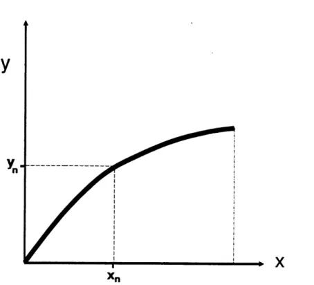
y

Yn

x

Xn

Figure 2.6: Coordinate System for a Cross-Section of the Nose Cone

(with RA = 0 for a cone), and of a cylinder by

S'yu = 2irRL.

If an equation is input, it is of the form y = f(x), as defined by Figure 2.6. Given the derivative, it is now solved numerically by integrating the following equation:20

S = |2ry + ddx

When a series of data points (x, yn) are entered, they are integrated around the x-axis using

i=n

S = 2 r yi ds i=l

2 0

where ds is the distance between two data points. Thus, given a value of S for the

nose cone, the mass can be estimated using

M

where = the half angle of the nose cones, Msat = the mass of the equivalent

Chapter 3

Reentry Heating

3.1 Introduction

The JRB is designed to be completely reusable with virtually no refurbishment required. As such, it must be able to withstand a fall from the height of separation

with the core to impact with the ocean. It is assumed that a parachute, ballute, or attitude control system will stabilize the body so that it passes through the

atmosphere nose-first. Though a deployable decelerator will be used to decelerate

it to less than 80 ft/sec at impact, this decelerator cannot be deployed until after

peak heating and deceleration loads have occured. This means that the booster, and specifically the nose cone (on which the stagnation-point is located), must be able to withstand the full effects of atmospheric heating. This can only be accomplished with certain geometries of the nose cone.

3.2 The Reentry Scenario

3.2.1

Environment

As the vehicle reenters the atmosphere, it passes through a number of flow regimes as the atmospheric density increases. The first regime is that of free molecular flow. With )A = mean free path and R = radius of the reentry body, this regime occurs when A > R so that gas phase collisions can be ignored. The near free molecule regime begins at an altitude of about 450 kftl, and is where molecular collisions begin to have an effect. From just over 400 kft to about 350 kft there is a transitional layer, below which are the continuum regimes. Cox and Crabtree [13] next define the fully merged layer, incipient merged layer, and vorticity interaction regimes, however they can be considered together (as in Martin [18]) as the viscous merged layer. Located from about 350 kft to 250 kft, this layer is characterized by viscous flow and the creation of a shock wave and boundary layer around the body. Below about 250 kft continuum flow is encountered. In this region normal high Reynolds number aerodynamics is valid, and the shock wave and boundary layer can be analyzed as a discontinuity.

In the first two flow regimes heat transfer rates are obtained from kinetic theory, using momentum and energy exchange accomodation coefficients [13, p. 216]. In the near free molecular flow regime the effect of molecules reemitted from the body

'For a more exact definition of the location of each flow regime, which are dependent on velocity and nose radius, see Chapter 9 in Reference [13].

striking other molecules in the fluid must be taken into account. These effects, however, are minor compared to those that occur in the lower regimes. As stated in [19, p. 12-02], "Almost all the critical heat transfer problems that arise in penetrating a planetary atmosphere occur in the continuum flow regime." Here, if the body is blunt, there is a detached shock wave behind which a layer of dissociated

and ionized gas occurs. This gas transfers heat to the vehicle through radiation.

There is also a boundary layer formed by fluid viscosity around the surface of the body. Here both conduction and diffusion transfer heat into the body. Heat is also radiated from the vehicle. Each of these heating methods are discussed in the next section.

3.2.2

Heating

Radiative heating is caused by energy emitted as photons. Radiation both transfers heat to the vehicle from the gas behind the shock wave and transfers heat from the vehicle back out to the atmosphere. The former can be approximated at the

stagnation-point in Btu/ft2_{-sec by using the following equation from Reference [19]:}

)

P~

130 vI 12.5

q ad-r x 1.3 3(-p-

)(V

where r = nose radius of the reentry body in feet, V = free-stream velocity in

ft/sec, p = free-stream density, and p = the density behind the normal shock

law:

= EoT4all,

where = emissivity of the body, = Stefan-Boltzman constant, and Tal = temperature of the body.

Convective heat transfer is caused by the bulk fluid motion in the boundary layer, giving rise to kinetic, rotational, and vibrational energy, much of which becomes heat. Also, heat conduction occurs as atoms and ions diffuse across the boundary layer, due to the large entropy change, and give up their chemical energy [18, p. 94]. In Reference [19] these effects are combined in a formula which is then simplified to

yield the following equation for the convective heat transfer at the stagnation point

(in English units):

3

21.9Vp 00( ₁₀₀₀V.XO

)

The JRB will reenter at a speed of 13,800 ft/sec at an altitude of 200 kft. According to Allen and Eggers [20, p. 7], the maximum stagnation point heat flux then occurs at an altitude of 117 kft and a velocity of 11,680 ft/sec.2 Using the

1976 U.S. Standard Atmosphere [21], at this altitude p, = 1.48 x 10- 5 slug/ft3. The stagnation density ratio at this altitude and velocity is found from Figure 2-9 in Reference [18] to be poo/po = .094. Using a value of Ro = 6ft,3 Equation 3.1 gives qrad = 2.57 Btu/ft2-sec and Equation 3.2 gives q, = 54.9 Btu/ft2_{-sec. Since}

2

These values come from Equations 3.8 and 3.9, and assume a CD of .5.

3

qrad/qo = .047, the radiation heating can be ignored in favor of the convective heating. This conclusion is further supported by the fact that convective heating is only a function of V, whereas radiative heating is a function of V.2 5, so as further deceleration occurs the ratio will become much more pronounced. For example,

at the point of maximum average heat flux per unit area,4 Qrad/q4, = 9.82 x 10-3, and at the point of maximum deceleration and the maximum altitude rate of heat

transfer,5 qrad/4.o = 1.97 x 10-3. As shown in References [22] and [19], it is only

for high speeds like those of planetary probes that radiative heating needs to be considered.

3.3 Minimum Heating Shapes

Prior to 1951 all rockets and missiles were designed with slender shapes in order to minimize pressure drag [23]. As pointed out by Lees [19], a vehicle returning from orbit has a kinetic energy of motion equivalent to 13,500 Btu's per pound. By the time this vehicle impacts the earth it will have converted almost all of this energy into heat. Since there is no material which can take this much heat, much of it must be used to heat the atmosphere. It was this latter conclusion that H. Allen, working at the NACA Ames Aeronautical Laboratory, came up with in 1951. By making

4Allen and Eggers [20, p. 6] derive this as occuring at an altitude of lIn( 23CDnA ) and a velocity AX 2M sin nd velocity of VEe- .

5_{Allen and Eggers [20, pp. 4 & 6] state that both these effects occur at an altitude of}

the vehicle blunt, the shock wave stand-off distance-increases and there is a greater

volume of air behind the shock wave to become heated. These results were formally published in Allen's joint paper with Eggers entitled "A Study of the Motion and Aerodynamic Heating of Ballistic Missiles Entering the Earth's Atmosphere at High Supersonic Speeds" [20].

This paper begins with a trajectory analysis, the results of which are used in the heating equations. These results are also used in Reference [24]. The basic assumptions taken include a constant coefficient of drag, no gravity term,6 _{and an}

exponential relationship between density and altitude. The results of this trajectory

analysis are integrated in heating equations to obtain the following equation for total

heat input:

1 S C po A

Q = ( _{4 CA} )MV(1 - e XMineE (3.3)_(3.3)

Here A = 221O ft-l and po = .0034 slugs/ft3. Since for a relatively light vehicle7 CDPOA

1 - e-is B 1

the heating is proportional to

CfS shearforce CDA dragforce

Thus Allen and Eggers were the first to show that increasing the pressure drag by

'The gravity term is commonly neglected in the literature, since with aerodynamic decelerations of 20 to several hundred g's, it has very little effect.

7_{For the JRB, a 100 nose cone (CD x .1) gives e-r cI~; 1 x 10}- _{, whereas a 300 nose cone} (CD_ OA 1 x 10

increasing the tip radius and cone angle will reduce the aerodynamic heating on the vehicle. However, Equation 3.3 cannot be used to obtain a numerical solution because the "equivalent skin friction coefficient" [20, p. 6] is left in the form

C = S

C p)(V)dS.

(3.4)

Several studies on the exact shape of minimum heat transfer bodies have been done, but Baker and Kramer were the first to compute such a shape for the heat-ing over an entire reentry trajectory environment. Their results are presented in Reference [25]. In this paper they use heat transfer equations they derived in Ref-erence [24] by starting with equations for local heat transfer coefficients for laminar and turbulent flow from Vaglio-Laurin's work (References [26] and [27]).These equa-tions are made non-dimensional, and then, following Allen and Eggers, an equation

for dQ/dy is obtained (using the approximation dy/dt = -V sin OE) where y is the altitude. This equation is integrated over the trajectory using the approximations

-Xy

Poo = poe

and

CDPO A -y

V = VEe 2AN " ""i (3.5) from Allen and Eggers. However, in Allen and Egger's analysis they assumed the shock-layer Reynolds number Re, was constant, and Baker and Kramer used