HAL Id: hal-02091102
https://hal.archives-ouvertes.fr/hal-02091102
Preprint submitted on 5 Apr 2019
HAL is a multi-disciplinary open access
archive for the deposit and dissemination of
sci-entific research documents, whether they are
pub-lished or not. The documents may come from
teaching and research institutions in France or
abroad, or from public or private research centers.
L’archive ouverte pluridisciplinaire HAL, est
destinée au dépôt et à la diffusion de documents
scientifiques de niveau recherche, publiés ou non,
émanant des établissements d’enseignement et de
recherche français ou étrangers, des laboratoires
publics ou privés.
Stacked Sparse Blind Source Separation for Non-Linear
Mixtures
Christophe Kervazo, Jerome Bobin
To cite this version:
Christophe Kervazo, Jerome Bobin. Stacked Sparse Blind Source Separation for Non-Linear Mixtures.
2019. �hal-02091102�
Kervazo C.1 Bobin J.1
Abstract
Linear Blind Source Separation (BSS) has known a tremendous success in fields ranging from biomedical imaging to astrophysics. In this work, we however propose to depart from the usual linear setting and tackle the case in which the sources are mixed by an unknown non-linear function. We propose a stacked sparse BSS method enabling a sequential decomposition of the data through a linear-by-part approximation. Beyond separating the sources, the introduced StackedAMCA can under discussed conditions further learn the inverse of the unknown non-linear mixing, enabling to reconstruct the sources despite a severely ill-posed problem. The qual-ity of the method is demonstrated on two experi-ments, and a comparison is performed with state-of-the art non-linear BSS algorithms.
1. Linear and Non-Linear BSS
1.1. Context
Since its formulation in the 1980s, Blind Source Separation (BSS) has become one of the major tools to learn meaningful decompositions of multivalued data. It is used in many fields, such as audio processing (Vincent et al.,2011;2003;
Ozerov & F´evotte,2010;Duong et al.,2010;F´evotte et al.,
2009), biomedical imaging (Jung et al.,2000;Negro et al.,
2016;Poh et al.,2010) or astrophysics (Bobin et al.,2014). Most of this work has however been dedicated to linear BSS, in which m observations are assumed to be the linear combinations of n sources, each of them having t samples. In matrix form, it is supposed that the data can be written as X = AS + N, with X (size m × t) the observation matrix corrupted with some unknown noise N. The sources S (n × t) are therefore supposed to be mixed linearly through the A matrix (m × n) and the goal of linear BSS is to
*
Equal contribution 1CEA Saclay, Gif-sur-Yvette, France. Cor-respondence to: Kervazo C. <[email protected]>. Proceedings of the35th
International Conference on Machine Learning, Stockholm, Sweden, PMLR 80, 2018. Copyright 2018 by the author(s).
recover both A and S from the sole knowledge of X up to a permutation and scaling indeterminacy. While linear BSS is ill-posed, several types of priors have been introduced to reduce the space of possible solutions. Among them, sparsity (Zibulevsky & Pearlmutter,2001) – which assumes that the sources have a large number of zero coefficients – has been shown to lead to enhanced separation quality on various problems of linear BSS (Bobin et al.,2008;2015;
Kervazo et al.,2018).
While convenient for many problems, the linear mixing model is only an approximation which might not hold in various experimental settings. For instance, it is not any-more valid when using sensors with saturations or non-linearities (for instance gas (Madrolle et al.,2018) or chem-ical (Jimenez,2006) sensors), or in some specific applica-tions (show-through removal (Merrikh-Bayat et al.,2011), hyperspectral imaging (Dobigeon et al.,2014)). In all these applications, it is therefore relevant to change the BSS model to a non-linear one:
X = f (S) + N (1)
Where f is an unknown non-linear function from Rn×tto
Rm×t. In this work, we will consider general functions f , by mostly (cf. Sec.4) assuming that f is invertible and symmetrical around the origin, as well as regular enough. Regular means that f is L-Lipschitz with L small enough and that f does not deviate from a linear mixing too fast as a function of the input amplitude. Furthermore, we will focus on the overdetermined case, in which n 6 m. At this point, it is important to mention that non-linear BSS is much more difficult than its linear counterpart and that it might not be possible to find both f and S up to a simple permutation and scaling indeterminacy. In the case of sparse sources, (Ehsandoust et al.,2016) has shown the possibility to recover the sources up to a nonlinear function if only one source is active for each sample. Therefore, the problem is too ill-posed to ensure a good reconstruction of the sources in the general case, and the goal of sparse non-linear BSS is only to separate the sources by estimating the underlying non-linearities.
1.2. Contribution
We propose to tackle the general problem of non-linear BSS presented in Eq. (1) by using a sparsity prior on the
sources. To the best of our knowledge, our method is the first attempting to find a linear-by-part approximation of the underlying non-linearities using a stacked sparse BSS approach. Beyond separating them, the algorithm proposes a possible reconstruction of the sources by inverting the es-timated linear-by-part model. Despite the usual non-linear BSS indeterminacies, the proposed reconstruction is empir-ically shown to estimate well the true sources under some discussed hypotheses. In Sec.2, the method is further de-scribed. In Sec.3, some experiments are conducted on two different mixings, and our method is compared to other ones to show its relevance. In Sec.4, the required hypotheses for the proposed approach are studied.
1.3. Previous Works
Among the different works dealing with sparse sources, many focus on specific mixing models: (Theis & Amari,
2004;Van Vaerenbergh & Santamar´ıa,2006;Duarte et al.,
2015) attempted the problem of Post Non-Linear (PNL) mixtures, and (Duarte et al.,2012) the problem of Linear-Quadratic (LQ) mixtures. General settings similar to the framework of the current article have mainly been studied in (Ehsandoust et al.,2016;Puigt et al.,2012). In these works, the approaches are however fully different since they are based on clustering algorithms.
It is also worth mentioning that the most comon approach is to use as prior the statistical independance of the sources instead of sparsity: this family of methods is known as Inde-pendant Component Analysis (ICA). Contrary to the linear case, this prior is nevertheless not anymore sufficient to sep-arate the sources in the general non-linear setting (Comon & Jutten,2010). Therefore, several kind of methods have emerged to bypass the separability issue. A first possibility is to explicitly focus on a special kind of mixing f (e.g. PNL and LQ mixtures – see (Deville & Duarte,2015)). Another possibility is to use an explicit or implicit regularization making the problem better posed. For explicit regularization, one can cite additional priors on the sources such as tempo-ral dependancies (Hyvarinen & Morioka,2017;Ehsandoust et al.,2017). Implicit regularization with specific separating algorithms can also be used, such as in (Almeida,2003;
Brakel & Bengio,2017;Honkela et al.,2007).
1.4. Notations
In this work, scalars are denoted as lower case letters (e.g. τ ), matrices in bold upper case letters (e.g. X), and their estimation by an algorithm as ˆX. The notation Xris the
line vector corresponding to the rth line of the matrix X
(X1..rbeing the set of lines from index 1 to r), while Xiis
the specific sample vector of Rmindexed by i. Functions with matrix outputs are written as f . In iterative algorithms, the estimate of a variable a at the lthiteration is denoted
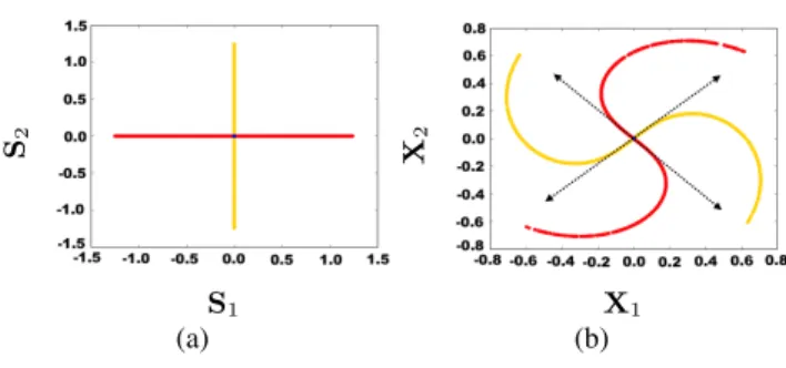
S1 S2 (a) X1 X 2 (b)
Figure 1. Left: Original sources; Right: A non-linear mixing of the left sources. The dashed arrows correspond to the mixing direc-tions found by a linear model.
Red color correspond to samples where S1is active and yellow to
samples where S2is active. These colors are displayed for
explan-ing the distortion introduced by the mixexplan-ing f but are unknown in a blind setting.
as a(l). The set of all the variables estimated between the iterations 1 to l is denoted as a(1..l).
2. Proposed Approach
2.1. A Geometrical Perspective on Sparse Non-Linear BSS
The proposed method is first discribed by adopting a geo-metrical point of view in the case n = 2; the generalization to higher values is in principle straightforward.
Due to the morphological diversity assumption (Bobin et al.,
2007), it is very rare that sparse sources both have non-zeros values at the same time. Therefore, when plotting the scatter plot of S1as a function of S2(cf. Fig.1(a)), most of the
source coefficients lie on the axes (in this work we even assume that all coefficients lie on the axes – this hypothesis is discussed in Sec.4). Once mixed with the non-linear f , the source coefficients lying on the axes are transformed into n non-linear one dimensional (1D) manifolds (Ehsandoust et al.,2016;Puigt et al.,2012), each manifold corresponding to one source (see Fig1(b)). To separate the sources, the idea is then to back-project each manifold on one of the axes. We propose to perform this back-projection by approximating the 1D-manifolds by a linear-by-part function, that we will invert. As evoked above, we then get separated sources which are only distorted through non-linear functions that do not remix them, called h in the following.
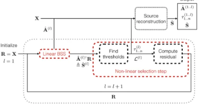
2.2. Overview of The Proposed Approach
As can be seen in Fig.1(b), the lowest amplitude data co-efficients can be well approximated by a classical linear model because of the regularity assumption on f , stating that the data must not deviate from linearity to fast as a
func-Figure 2. Main steps of StackedAMCA and corresponding nota-tions
tion of the amplitude. Finding such an approximation can in practice be done using a sparse linear BSS algorithm, provided that this one is robust to the higher amplitude non-linearities. A rough estimate of the sources can then be computed by inverting the found linear model. As expected, the corresponding separation is however very poor for the higher amplitude highly non-linear samples, as seen in3(a), where such samples (outside of the red square) do not lie at all on the axes as we would like. The question is then: how to better separate these samples? This is done by intro-ducing a non-linear selection step enabling to remove the contribution of the previously found linear model, creating a new dataset R comprehending only the highest non-linear samples, which amplitudes are further shrinked. Since the amplitudes are then smaller, working on R (cf. Fig.3(b)) makes possible the estimation of a new linear model that separates better the originally higher amplitude coefficients. It is then possible to repeat the procedure to improve the separation of still higher non-linear samples.
2.3. Detailled Description
2.3.1. DETAILSABOUT THEALGORITHMSTRUCTURE
As evoked in the previous subsection, computing a whole linear-by-part approximation of the 1D-manifolds is done iteratively. Each iteration l of the algorithm repeats the al-ternance explained above between the linear BSS step and the non-linear selection (thresholding) step. The first step computes a linear model ˆA(l) on the current residual R.
The second one paves the way for the next iterations by computing a new residual R. This is done by finding for each source r a maximum amplitude value τr(l)above which
the non-linearities are too high to be considered by currently well estimated, and then shrinking the current data using the τ1..n(l) (cf. Fig.3for one iteration). This shrinkage en-ables to sequentially reduce the amplitudes of the originally higher non-linearities, and therefore to compute linear mod-els describing them. The whole procedure, as well as some notations that will be developped in the following detailed
explanation of the two main steps, are summarized in Fig.2.
2.3.2. LINEARSPARSEBSS STEP: AMCA
The main requirement for the linear sparse BSS algorithm is its ablility to find a linear model representing well the lowest amplitude samples of the residual R, while being insensi-tive to the higher amplitude samples that are more affected by the non-linearities. Therefore, we use the Adaptative Morphological Component Analysis (AMCA - (Bobin et al.,
2015)) algorithm, which enables to separate sources hav-ing coefficients with both partial correlations (i.e. multiple sources are simultaneously active) and large amplitudes. In brief, AMCA introduces a way to discard the corresponding partially-correlated samples in the estimation process. Indeed, the problem of partial correlations and non-linear models both have in common that some samples with high amplitudes deviate from linearity. With a regular non-linear model, this is the case by definition. With a linear model, this is true in the sense that the activation of a second (or more) source causes a sample of the mixing to be outside the line drawn by the “pure”observations (i.e. steming from an unique source).
Therefore, in the case of non-linear models AMCA enables to discard the samples with high amplitudes that are the most affeted by the non-linearities, because these are considered as partial correlations. The algorithm is thus able to find a good linear model ˆA(l)of the lowest amplitude samples
of R, which is then inverted to align the lowest amplitude samples of each 1D-manifold with the axes. The result is denoted as: ˆS(l)
, ˆA(l)†r R (cf. Fig.3(a)).
2.3.3. SELECTIONFUNCTION: COMPUTINGR
The goal of the selection function is to extract within the sources ˆS(l)the contributions that are not explained by the linear model found with the BSS step. For finding such con-tributions, there are two issues: i) determine which samples are well separated by the current linear model ˆA(l); ii) actu-ally computeR by shrinking ˆS(l)to remove the contribution
explained by the current linear model.
Solution to problem i) StackedAMCA uses for each sample of ˆS(l)the distance (or more specifically the angle) to the
axes. If such a distance is small enough, it is assumed that the sample is well separated by the current linear model. We write L(l) the set of all such well separated samples.
Then, for each source k, the threshold τk(l)required for the amplitude shrinkage (see below) is roughly chosen as the maximum amplitude of the samples close enough to the axis of k (e.g. the ones in L(l) and generated by k – see
Fig.3(a)).
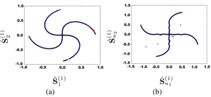
ˆ S(1)1 (a) R1 R 2 (b)
Figure 3. Illustration of the main steps of the algorithm on the non-linear mixing of Fig.1. Upper left: in blue, output of linear BSS step: S(1)is displayed. Compared to Fig.1(b), inverting the lineart model corresponds to align the found dashed arrows of Fig.1(b)with the axes. In addition, the red square delimits the low amplitude sample areas of of S(1)where the linear model is a
good approximation – the corresponding maximum amplitudes are denoted by τ1..n(1) – which means the areas where the points almost
lie on the axes; Down right: Residual R after the selection step. In brief, removing the contribution of the found linear model is done by shrinking the amplitudes of the samples in X by τ1..n(1).
τ1..n(l) , ˆS(l)must be shrinked correspondingly, which is not trivial. To understand how such a shrinking works, we will focus on one specific sample ˆSi(l)
∈ Rn(i ∈ [1, t]) of ˆS(l)
that was generated with only the source r active (which we do not know in advance in the blind unmixing). We can differentiate two cases:
• ˆSi(l)∈ L(1..l), which means that ˆSi(l)is a point inside
the red square in Fig.3(a). Therefore, ˆSi(l)has been
separated by the linear-by-part model in the current or previous iterations. The separation is already per-formed and there is nothing left to do: Ri is set to a
vector with only zero coefficients.
• ˆSi(l) ∈ L/ (1..l), which means that ˆSi(l) is a point
out-side the red square in Fig.3(a). The sample Rishould correspond to ˆSi(l) with the rthcoefficient having its
amplitude shrinked by τr(in Fig.3(a), we have to make
the samples outside the red square closer to the origin by removing the red square contribution). Choosing which threshold among the τ1..n to apply is however
nota trivial issue, because ˆSi(l)has not been fully
un-mixed by the linear-by-part model yet and we thus do not know by which source it was generated. There-fore, we will resort to a first guess to attribute ˆSi(l)to a source ˆr, hoping that ˆr = r. The idea is that even if ˆSi(l) has not been fully unmixed yet, we can still use the linear models computed during the previous iterations to improve the guess about ˆr. To do that, we start from the raw data X and iteratively unroll the manifold by sequentially applying the inverse of the previously computed linear models ˆA(1..l)and τ(1..l)
ˆ S(1)1 ˆ S (1) 2 (a) ˆ S(1)u1 ˆ S (1) u2 (b)
Figure 4. Illustration of the interest of unfolding the manifold to enhance the first guess about the unmixing of samples. A given sample is plotted in red. Left: data aligned with the axes corre-sponding to the sources; Right: Unrolled manifolds at the iteration l = 3. The sample in red is much closer to the good source, enabling to use simply an angular distance to the different axes.
(cf. Fig4). There are two advantages of this procedure: a) using the raw data X enables to get rid of the error propagation due to bad first guesses in the previous iterations; b) it is likely to make the sample indexed by i closer to the axes and thus a simple distance to the axes will hopefully enable to find a decent guess ˆr (cf. Fig4, where the position of one specific sample is shown, both in the scatter plot of X and in the unrolled manifold). The shrinkage of sample i is then done by thresholding the ˆrthcoefficient accordingly to τ
ˆ r.
Computing the whole residual will sum up to apply the process to all the samples in ˆS(l). The result of the shrinkage
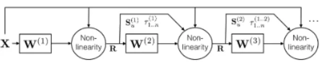
is then used as residual R in the following iterations. 2.4. Neural Network Interpretation
StackedAMCA can be interpreted as the multilayer neural network of Fig.5. The different network layers then exactly correspond to the iterations l. Such an interpretation is use-ful for understanding StackedAMCA: each layer computes a linear approximation of some part of the data.
Slightly altering the notations and writing W(l) = ˆA(l)†,
with the † sign corresponding to the pseudo-inverse, each neuron layer corresponds to the estimate ˆA(l)yielded by the
linear BSS step. In Fig.5, the non-linear step corresponds to the residual computation. Here, we again extended our notations, introducing the matrix Sucorresponding to the
unfolded manifold. Due to the thresholding, this step is very similar to classical non-linearities in neural networks such as the Rectified Linear Unit (ReLU - (Maas et al.,2013)). The network thus possesses the classical alternance between neuron layers and non-linearities. We further need skip connections to complete the transcription of the algorithm. In particular, these enable to re-use X directly, reducing the error propagations and improving the results similarly as
Figure 5. StackedAMCA as neural network
usual skip connections (Huang et al.,2017)).
However, contrary to many learning processes the layers are trained one-by-one, each of them minimizing the cost function of AMCA (Bobin et al.,2015), which would corre-spond to a greedy training. A global refinement step could however be added. One of the main differences is also that the thresholds τ1..n(1..l)are not learnt by minimizing a global cost function through backpropagation but roughly speaking directly from the data itself.
3. Experiments
We propose to demonstrate the relevance of the method with two experiments, after first presenting the metrics used to measure the result quality and introducing a new one for the case of sparse sources.
3.1. Metric
Due to the indeterminacy by the non-linear function h in non-linear BSS, it is important to differentiate measures about the reconstruction of the sources and their separation. 3.1.1. METRIC FOR THESEPARATIONQUALITY
A classical approach to determine the separation quality is to draw the scatter plot of each estimated source ˆSras
a function of the true one Sr (cf. Fig.9). If the sources
are perfectly separated, the plot should be a non-linear 1D function corresponding to h (Ehsandoust et al.,2017). Some possible metrics are therefore computed by fitting a non-linear curve P to the 1D-manifold of the scatter plot (by hoping that it will represent h) and looking at the thickness of the manifold around this non-linear curve. Here, the thickness will be measured in two different ways (once the permutations between ˆS and S are corrected):
• Looking at the median distance with the curve P:
Cmed=P
n
r=1mediani(ˆSir− P(Sir))
• Looking at the squared distance with the curve P: Csq=P n r=1 1 t q Pt i=1(ˆSir− P(Sir))2
However, the results of these metrics are sensitive to the choice of P (and more specifically its smoothness). We thus propose to introduce a new metric based on the angular distance to the axes: if the sources are perfectly separated,
their scatter plot should resemble the one from Fig.1(a), the samples lying on the axes. We can therefore estimate the separation quality of each source ˆSrby looking at its scatter
plots as a function of the true other sources Sr0, r0 6= r, and
looking at the average angles of the samples with the axes. More specifically, the metric we use is:
Cang= 1 n(n − 1) n X r=1 n X r0 =1 r0 6=r 1 − 1 #Z X t∈Z St r0 q ˆ St2 r + St 2 r0 (2) where Z = {t|Str0 6= 0} and #Z denotes the cardinal of Z.
3.1.2. METRICS FORSOURCERECONSTRUCTION
To determine whether the source reconstruction is good or not, it is possible to use classical metrics between the estimated and true sources, such as the Mean Squared Error (MSE), the Mean Error (ME), the SDR (Vincent et al.,2006). Lastly, in the first experiment where f is linear-by-part, it is straightforward to use linear BSS metrics on each part, such as the mixing criterion CA(Bobin et al.,2008).
3.2. Linear-By-Part Mixing
In this first experiment, the mixing is created as linear-by-part, thus perfectly matching the unmixing process of StackedAMCA. Therefore, the algorithm should by con-struction work well and be able to reconstruct well the sources. This experiment should further enable to study its main mechanisms. More specifically, the sources have t = 10000 samples, with disjoints support and a sparsity level of p = 10%. There is m = n = 2 observations, which are created with a linear-by-part f , for which each part corresponds to an orthogonal A(l)matrix. The data X is shown in Fig.6(while the linear-by-part mixing might seem simplistic, the current mixing however deviates much from the linearity). In this experiment, both the mixing matrices A(1..l) and the optimal thresholds are knwown, which enables to assess the quality of their estimation by StackedAMCA.
3.2.1. NOISELESSMIXING
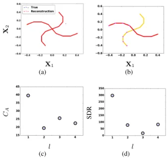
In this part we deal with the noiseless setting, in which the algorithm should be able to work well. The first evaluation is qualitative. An easy verification is to check that the learnt model can reconstruct the data. Figure7displays the recon-structed data superimposed on the true one and show that except for 2 outliers (likely to come from a thresholding in the wrong direction), the reconstruction is almost per-fect. This however does not guarantee the separation of the sources. Fig.7therefore displays the scatter plot of the data X with colors corresponding to the different sources: each manifold is labeled with only one source.
X1 X 2 (a) X1 (b)
Figure 6. Two datasets X corresponding to two different non-linearities f . Left: linear-by-part mixing; Right: Star mixing.
Table 1. Different metrics on the whole sources in the noiseless and noisy experiment. The last line corresponds to an Euclidian distance between the optimal thresholds and the estimated ones.
SETTING NOISELESS NOISY
CA 22.5 23.6
SDR 23.4 6.83 ERROR ONτ1..n(1..l) 4.86 × 10⁻³ 9.20 × 10⁻²
To quantitatively assess the results of StackedAMCA, Ta-ble1presents a few metrics about the whole sources. The quite high CAconfirms that the separation is good, while
the decent SDR shows that despite the non-linear setting, the source reconstruction is decent. Moreover, Fig.7displays the evolution of these metrics as a function of the iterations. The good results for the first iteration indicates as expected that AMCA is robust enough to discard the highly non-linear high amplitude coefficients. There is then a general decrease of both CAand the SDR with the iteration number, which
is however not strictly monotonic as expected, probably due to the fact that some errors done at a given layer l can be compensated at the following layer (e.g. by still finding the good thresholds τ1..n(l+1)).
3.2.2. NOISYMIXING
Compared to the previous experiment, a noise N correspond-ing to a Signal-to-Noise Ratio of SNR = 30dB is added to the mixing. While we do not aim at re-doing the whole study of the previous subsection, two interesting plots are displayed in Fig.8. In left, it is shown that more outliers appear in the data reconstruction. This is explained by the right plot where a part of source 1 has been mixed with source 2 (red samples in the yellow part of the manifold). Furthermore, Table 1shows that while the separation is globally (except the few outliers) good as testified by CA,
the SDR expresses a quite bad reconstruction whereas the structure of the mixing f should enable StackedAMCA to reconstruct well the sources. The bad source reconstruction
X1 X 2 (a) X1 (b) l CA (c) l SDR (d)
Figure 7. Upper left: Reconstruction of the data from the model estimated by StackedAMCA, superimposed on the true data X; Upper right:True data, with the colors coming from the demixing: red corresponds to source one and yellow to source two. Points in violet correspond to the samples used to compute the thresholds τ1..n(1..l); Down left: CAas a function of the iteration l; Down right:
SDR as a function of l.
is rather explained by bad thresholds τ1..n(1..l), as shown by the violet points of the right plot of Fig.8, to be compared with its counterpart in the noisless setting in Fig.7. This is confirmed by the last line of Table1. Wrong τ1..n(1..l)create wrong offsets between the linear parts, creating a shift in some samples of ˆS and therefore explaining a deteriorated source reconstruction. Still robustifying the threshold choice is left for future works.
3.3. Star Mixing: Comparison to Other Methods The goal of this part is to compare the results of our al-gorithm to other existing ones. Only a few alal-gorithms for non-linear BSS are open source, and we mostly found three of them: MISEP (Almeida,2003), NFA (Honkela et al.,
2007) and ANICA (Brakel & Bengio,2017). The exper-iment itself comes from (Ehsandoust et al.,2016). The sources follow a Bernouilli-Gaussian ditribution, p = 10% of the t = 9500 samples being non-zeros. The supports of the n = 2 sources are disjoint. There is m = n = 2 observations, which are computed for each element indexed by i ∈ [1, t] as Xi
1 = cos(α(i))Si1− sin(α(i))Si2+ Ni1
and Xi2 = sin(α(i))Si1+ cos(α(i))Si2+ Ni2with α(i) =
π 2(1 − q Si2 1 + Si 2
2) and N chosen such that the SNR is 30
X1 X 2 (a) X1 (b)
Figure 8. Left: Reconstruction of the data from the model esti-mated by StackedAMCA, superimposed on the true data X; Right: True data, with colors coming from the demixing. Points in violet correspond to the samples used to compute the thresholds τ1..n(1..l).
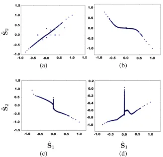
Different separation metrics are displayed in Table2and the reconstruction quality is assessed in Table3. The cor-responding results are shown in Fig.9, where the scatter plot of one estimated source is drawn as a function of the true one. First, it seems that neither ANICA nor NFA truly separate the sources (concerning ANICA, the results seem however to improve when no noise is added). Although it could come from our lack of familiarity with the parameter tuning of these methods, it is possible that the regularization introduced by the network structure for ANICA and the Bayesian setting for NFA is not sufficient to enable the sepa-ration of the sources (since the independance is not either, cf. Sec1). On the contrary, MISEP separates the sources well. Its results are even better than the ones of StackedAMCA when measured with a squared distance Csq, which is due
to the presence of a small number a very badly separated samples with StackedAMCA. These outliers probably come from residual error propagation due to the temporary un-mixing of the manifold (cf. Sec.2). Using metrics that are less sensitive to outliers shows that the other samples are hower much better separated by StackedAMCA: Cmedis
reduced by 10 compared to MISEP. The good separation of StackedAMCA is confirmed by the best Cang.
Second, MISEP does not reconstruct well the sources as StackedAMCA does and Fig.9(b)clearly indicates that it did not invert the non-linearity h. On the contrary, the good ME (and even MSE, depite some outliers) of StackedAMCA indicates that the algorithm structure was sufficient to regu-larize well the reconstruction problem. Some non-linearities f for which StackedAMCA is able to perform such a good reconstruction are characterized in Sec.4.
4. Required Hypotheses for StackedAMCA
4.1. Symmetry of f Around the Origin
The symmetry assumption could in principle be leveraged. First, the data can be symmetrical around a different point as
Table 2. Separation quality of 4 methods: StackedAMCA, MISEP, NFA and ANICA. The curve P fitted to the scatter plots displayed in Fig.9is chosen as a polynomial function of degree 20.
METHOD Cmed Csq Cang
STACKEDAMCA 1.42 × 10⁻⁴ 3.17 × 10⁻⁴ 3.69 × 10⁻³ MISEP 4.25 × 10⁻³ 6.58 × 10⁻⁵ 1.49 × 10⁻² NFA 4.60 × 10⁻² 1.12 × 10⁻³ 0.273 ANICA 2.00 × 10⁻² 5.67 × 10⁻⁴ 0.699
Table 3. Reconstruction quality of 4 methods: StackedAMCA, MISEP, NFA and ANICA.
METHOD MSE ME
STACKEDAMCA 2.45 × 10⁻⁴ 6.70 × 10⁻⁴ MISEP 7.35 × 10⁻⁴ 1.72 × 10⁻² NFA 1.56 × 10⁻³ 6.67 × 10⁻² ANICA 2.25 × 10⁻² 2.10
long as a preprocessing step is introduced to center it. Then, tackling non-symmetrical data could probably be dealt with by introducing non symmetrical non-linear steps and adding a non-negativity constraint in the linear BSS step.
4.2. Disjoint Supports
We have assumed the supports of the sources to be dis-joint. While this is not very realistic in practical cases, it seems difficult to bypass this condition as we only explore the span of f that the 1D-manifolds created by the sparse sources uncover. By the morphological diversity assump-tion, the points outside these manifolds are too rare to enable a proper estimation of f without any further conditions (e.g. the separability over the different sources). We however emphasize that we did some tests without disjoint supports. In this case, the samples with multiple active sources were badly separated but the estimation of the 1D-manifolds by StackedAMCA was not much perturbated, which is mainly due to the robustness of AMCA to multiple active sources. 4.3. Regularity of the Mixing f
We have assumed that f does not deviate too fast from lin-earity as a function of the amplitude. For differentiable curves, it mathematically means that at every point of the 1D-manifolds described by the mixing X, the local cur-vature radius must be large enough. This condition is of primary importance to enable StackAMCA to separate the sources. This can be understood with the counterexample of a linear-by-part f (similarly as in Fig.6) with two parts. If A(1)is the identity matrix and A(2)a rotation matrix with
itera-ˆ S2 (a) (b) ˆ S1 ˆ S2 (c) ˆ S1 (d)
Figure 9. Scatter plot of one estimated source as a function of the true source. Upper left: StackedAMCA; Upper right: MISEP; Down left:NFA; Down right: ANICA.
tion will introduce a permutation between the sources of the first and second layer, thus yielding an imperfect separation. For a similar permutation reason between the iterations, f must also be L-Lipschitz with L small enough. In brief, this is due to the fact that AMCA is initialized at each iteration l+ 1 with the mixing matrix estimated at the previous iteration l. Consequently, AMCA looks for a similar matrix, which corresponds to looking for a slowly varying mixing f . 4.4. What Sources can StackedAMCA Reconstruct
Well?
In Sec.3, StackedAMCA was able to reconstruct the sources well. Due to the indeterminacy by h, it is however not always be the case, as demonstrated in Fig. 10 where a slight modification of the mixing f of Sec. 3makes that StackedAMCA is not anymore able to fully invert the non-linearity (while still decently separating the sources). While other methods (such as MISEP or ANICA) are also able to perform the reconstruction of the sources for some specific mixings, a very interesting point is that it is further possible to characterize at least one type of mixings for which StackedAMCA is able to approximately reconstruct the true sources up to a simple scaling and permutation indeterminacy. Indeed, a sufficient condition is that for each sample of the mixing indexed by i, the mixing f can be written as a product of an unitary matrix and the sources:
G = {f : Rn×t→ Rm×tk∀i ∈ [1, t], Xi= A(Si) Si, A(Si) ∈ O} (3) X1 X 2 (a) ˆ S1 ˆ S2 (b)
Figure 10. Example in which StackedAMCA is not anymore able to reconstruct the sources. The mixing is chosen so that for all i ∈ [1, t], Xi1 = cos(α(i))r(i)Si1− sin(α(i))Si2 and Xi2 =
sin(α(i))r(i)Si
1+cos(α(i))Si2with α(i) =π2(1−
q Si2 1 + Si 2 2) and r(i) = q Si2 1 + Si 2
2. Left: Mixing; Right: Results of
StackedAMCA for source 1.
where O is the oblique set (that is, the set of matrices with unitary columns). The function A(.) : Rn → Rm×n is
potentially non-linearly depending on S. Then, if f ∈ G and also follows the other assumptions of this article, the mixed sources can be approximately reconstructed by StackedAMCA. Indeed, since in AMCA the scale of the matrices A(l)is fixed to 1, if f ∈ G there is no ambiguity left for the scale of each layer. Due to the regularity assump-tion, it will then be possible to backproject linearly for each layer the manifold on the axes with small errors and get an approximatereconstruction.
5. Conclusion
We introduce in this work StackedAMCA, a new algorithm tackling the sparse non-linear BSS problem. Based on a new stacked sparse BSS approach, this method enables to sequentially compute a linear-by-part approximation of the underlying non-linearities. Each linear part is estimated by a robust linear BSS algorithm step, which is followed by a non-linear step . The non-linear step enables to work on in-cresingly higher non-linearities and is itself composed of an unrolling of the source 1D-manifolds and then a threshold-ing. We show the relevance of StackedAMCA compared to other state-of-art methods. Beyond separating the sources, in some experiments the algorithm is also able to reconstruct them well despite a severly ill-posed problem. A discus-sion of the required hypotheses for StackedAMCA to work is furthermore proposed, as well as a characterization of some datasets for which it should be able to reconstruct the sources well. An improvement left for future work, that should in principle be straightforward, is the extension of the algorithm to more than two sources.
References
Almeida, L. B. Misep–linear and nonlinear ica based on mu-tual information. Journal of Machine Learning Research, 4(Dec):1297–1318, 2003.
Bobin, J., Starck, J.-L., Fadili, J. M., and Moudden, Y. Sparsity and morphological diversity in blind source sep-aration. IEEE Transactions on Image Processing, 16(11): 2662–2674, 2007.
Bobin, J., Starck, J.-L., Moudden, Y., and Fadili, M. J. Blind source separation: The sparsity revolution. Advances in Imaging and Electron Physics, 152(1):221–302, 2008. Bobin, J., Sureau, F., Starck, J.-L., Rassat, A., and Paykari,
P. Joint PLANCK and WMAP CMB map reconstruction. Astronomy & Astrophysics, 563:A105, 2014. Bobin, J., Rapin, J., Larue, A., and Starck, J.-L. Sparsity and
adaptivity for the blind separation of partially correlated sources. IEEE Transanctions on Signal Processing, 63 (5):1199–1213, 2015.
Brakel, P. and Bengio, Y. Learning independent features with adversarial nets for non-linear ICA. arXiv preprint arXiv:1710.05050, 2017.
Comon, P. and Jutten, C. Handbook of Blind Source Separa-tion: Independent component analysis and applications. Academic Press, 2010.
Deville, Y. and Duarte, L. T. An overview of blind source separation methods for linear-quadratic and post-nonlinear mixtures. In International Conference on La-tent Variable Analysis and Signal Separation, pp. 155– 167. Springer, 2015.
Dobigeon, N., Tourneret, J.-Y., Richard, C., Bermudez, J. C. M., McLaughlin, S., and Hero, A. O. Nonlinear un-mixing of hyperspectral images: Models and algorithms. IEEE Signal Processing Magazine, 31(1):82–94, 2014. Duarte, L. T., Ando, R. A., Attux, R., Deville, Y., and
Jutten, C. Separation of sparse signals in overdetermined linear-quadratic mixtures. In International Conference on Latent Variable Analysis and Signal Separation, pp. 239–246. Springer, 2012.
Duarte, L. T., Suyama, R., Attux, R., Romano, J. M. T., and Jutten, C. A sparsity-based method for blind compensa-tion of a memoryless nonlinear distorcompensa-tion: Applicacompensa-tion to ion-selective electrodes. IEEE Sensors Journal, 15(4): 2054–2061, 2015.
Duong, N. Q., Vincent, E., and Gribonval, R. Under-determined reverberant audio source separation using a full-rank spatial covariance model. IEEE Transactions on Audio, Speech, and Language Processing, 18(7):1830– 1840, 2010.
Ehsandoust, B., Rivet, B., Jutten, C., and Babaie-Zadeh, M. Nonlinear blind source separation for sparse sources. In Signal Processing Conference (EUSIPCO), 2016 24th European, pp. 1583–1587. IEEE, 2016.
Ehsandoust, B., Babaie-Zadeh, M., Rivet, B., and Jutten, C. Blind source separation in nonlinear mixtures: separabil-ity and a basic algorithm. IEEE Transactions on Signal Processing, 65(16):4339–4352, 2017.
F´evotte, C., Bertin, N., and Durrieu, J.-L. Nonnegative matrix factorization with the Itakura-Saito divergence: With application to music analysis. Neural computation, 21(3):793–830, 2009.
Honkela, A., Valpola, H., Ilin, A., and Karhunen, J. Blind separation of nonlinear mixtures by variational bayesian learning. Digital Signal Processing, 17(5):914–934, 2007.
Huang, G., Liu, Z., Van Der Maaten, L., and Weinberger, K. Q. Densely connected convolutional networks. In 2017 IEEE Conference on Computer Vision and Pattern Recognition (CVPR), pp. 2261–2269. IEEE, 2017. Hyvarinen, A. and Morioka, H. Nonlinear ICA of
tem-porally dependent stationary sources. Proceedings of Machine Learning Research, 2017.
Jimenez, G. B. Non-linear blind signal separation for chem-ical solid-state sensor arrays. PhD thesis, Universitat Polit`ecnica de Catalunya, 2006.
Jung, T.-P., Makeig, S., Humphries, C., Lee, T.-W., Mck-eown, M. J., Iragui, V., and Sejnowski, T. J. Removing electroencephalographic artifacts by blind source separa-tion. Psychophysiology, 37(2):163–178, 2000.
Kervazo, C., Bobin, J., and Chenot, C. Blind separation of a large number of sparse sources. Signal Processing, 150: 157–165, 2018.
Maas, A. L., Hannun, A. Y., and Ng, A. Y. Rectifier non-linearities improve neural network acoustic models. In Proc. icml, volume 30, pp. 3, 2013.
Madrolle, S., Grangeat, P., and Jutten, C. A linear-quadratic model for the quantification of a mixture of two diluted gases with a single metal oxide sensor. Sensors, 18(6): 1785, 2018.
Merrikh-Bayat, F., Babaie-Zadeh, M., and Jutten, C. Linear-quadratic blind source separating structure for removing show-through in scanned documents. International Jour-nal on Document AJour-nalysis and Recognition (IJDAR), 14 (4):319–333, 2011.
Negro, F., Muceli, S., Castronovo, A. M., Holobar, A., and Farina, D. Multi-channel intramuscular and surface EMG decomposition by convolutive blind source separation. Journal of neural engineering, 13(2):026027, 2016. Ozerov, A. and F´evotte, C. Multichannel nonnegative matrix
factorization in convolutive mixtures for audio source separation. IEEE Transactions on Audio, Speech, and Language Processing, 18(3):550–563, 2010.
Poh, M.-Z., McDuff, D. J., and Picard, R. W. Non-contact, automated cardiac pulse measurements using video imag-ing and blind source separation. Optics express, 18(10): 10762–10774, 2010.
Puigt, M., Griffin, A., and Mouchtaris, A. Nonlinear blind mixture identification using local source sparsity and functional data clustering. In Sensor Array and Multi-channel Signal Processing Workshop (SAM), 2012 IEEE 7th, pp. 481–484. IEEE, 2012.
Theis, F. J. and Amari, S.-i. Postnonlinear overcomplete blind source separation using sparse sources. In Interna-tional Conference on Independent Component Analysis and Signal Separation, pp. 718–725. Springer, 2004. Van Vaerenbergh, S. and Santamar´ıa, I. A spectral
clus-tering approach to underdetermined postnonlinear blind source separation of sparse sources. IEEE Transactions on Neural Networks, 17(3):811–814, 2006.
Vincent, E., F´evotte, C., Gribonval, R., Benaroya, L., Rodet, X., R¨obel, A., Le Carpentier, E., and Bimbot, F. A ten-tative typology of audio source separation tasks. In 4th Int. Symp. on Independent Component Analysis and Blind Signal Separation (ICA), pp. 715–720, 2003.
Vincent, E., Gribonval, R., and F´evotte, C. Performance measurement in blind audio source separation. IEEE transactions on audio, speech, and language processing, 14(4):1462–1469, 2006.
Vincent, E., Jafari, M. G., Abdallah, S. A., Plumbley, M. D., and Davies, M. E. Probabilistic modeling paradigms for audio source separation. In Machine Audition: Principles, Algorithms and Systems, pp. 162–185. IGI Global, 2011. Zibulevsky, M. and Pearlmutter, B. A. Blind source sep-aration by sparse decomposition in a signal dictionary. Neural Computation, 13(4):863–882, 2001.