DETAILED TIME RESOLVED MEASUREMENTS AND ANALYSIS OF UNSTEADY FLOW IN A
TRANSONIC COMPRESSOR by
WING FAI NG
GAS TURBINE
LIBRARY
DETAILED TIME RESOLVED MEASUREMENTS AND ANALYSIS OF UNSTEADY FLOW IN A
TRANSONIC COMPRESSOR by
WING FAI NG
2
ABSTRACT
Detailed time and space resolved measurements for a transonic compressor
stage have been completed in the MIT Blowdown Compressor Facility. The stage studied was a new first stage for a NASA two-stage machine which incorporated
low-aspect-ratio blading. This rotor has an inlet hub/tip ratio of 0.375,
aspect ratio of 1.56 and an inlet relative Mach number of 1.38. The purposes of the test were to compare the results obtained by the Blowdown technique
with those found by steady state testing at NASA Lewis Research Center, and
to provide new time resolved data on the blade-to-blade flow in the rotor and stator. Data were obtained by surveys with a five diaphragm high frequency
response probe and by tip casing transducers.
The stage was tested at 100% design speed. Time resolved estimates of
efficiency were obtained by direct measurement of stagnation pressure together
with calculation of stagnation temperature by the Euler equation using measured tangential flow Mach number. Test results showed that the rotor achieved an
adiabatic efficiency of 0.895 at a total pressure ratio of 1.677. The stage
achieved an adiabatic efficiency of 0.862 at a total pressure ratio of 1.658.
Corrected mass flow at design was measured to be 33.3 Kg/s with respect to air. Time averaged flow quantities in general agree very well with results from steady state tests at NASA Lewis Research Center. A significant
differ-ence was observed in the variation of efficiency with radius, with a low
efficiency region near mid-span not observed in the steady state testing.
Moreover, the measured rotor efficiency in the "core flow" between the blade wakes for the supersonic region is lower than can be explained by normal shock
losses. Large streamwise vorticity is observed at the blade trailing edge in the inner half of the annulus, which may be associated with shock termi-nation at the sonic radius.
AC KNOW LEDGEMENTS
The author would like to express his sincere appreciation to all of the members of the Gas Turbine Laboratory who contributed to this
work. Foremost among these is Prof-essor Jack L. Kerrebrock, without whose expertise on the subject, the completion would have been
impossible. He also provided much time and unending encouragement, both were of invaluable help.
Also many thanks are due to Professor Alan H. Epstein, whose
guidence was essential in all phases of the research.
Professor William T. Thompkins, Jr. deserves special thanks for providing many helpful suggestions during frequent discussions.
The typing skill of Holly Rathbun is greatly appreciated. Finally, the author dedicates this thesis to his late beloved Brother, whom he missed very much during his course of study at MIT.
This research was supported by NASA Lewis Research Center under Grant NGL-22-009-383.
4 TABLE OF CONTENTS CHAPTER NO. PA FIGURES REFERENCES I INTRODUCTION II THE EXPERIMENT A. Test Facility
B. Test Compressor & Operating Point C. Instrumentation
1. High Frequency Sphere Probe 2. Total Pressure Probe
3. Instrumentation Ports
4. Wall Static Measurement & Other Instrumentation D. Data Acquisition & Processing
III RESULTS
A. Description of Results 1. Probe Data Behind Rotor
2. Contour Plots of High Response Data 3. Probe Data Behind Stator
4. Wall Static Pressure Measurements B. Discussion of Results
1. Mass Flow Determination & Mach Number Measurements
2. Rotor Overall Performance
3. Stage Overa Il Performance
IV CONCLUSIONS GE NO. 10 12 12 13 14 14 17 17 18 18 20 20 20 25 28 31 33 33 35 37 39 41 120
LIST OF FIGURES FIGURE NO 2.1 2.2 2.3 2.4 2.5 2.6.A 2.6.B 2.7 2.8.A, & C 2.9 2.10 2.11 2.12 3.1 .A 3. .B 3. 1 .C 3.1 .D 3. 1 .E 3.1 .F 3. .G B, P Scale Drawing of Blowdown Compressor Facility
Scale Drawing of Test Section Showing Location of Instrumentation Ports and Stage Flowpath
Matching Between Rotor Deceleration & Change in
Supply Tank Temperature
Pressure Variation in Blowdown Facility at Different Locations
Scale Drawing of Rotor Blade Shape Picture of 5-Way Probe
Sketch of 5-Way Probe Showing Air Angle Definition
5-Way Probe Position Vs. Time During the Traverse
(Probe Behind the Rotor)
5-Way Probe Calibration Curve for Mach Number = 0.7 Flow Chart for 5-Way Probe Data Reduction
Scale Drawing and Picture of Miniature Stagnation Pressure Probe
Scale Drawing of Rotor Tip Section & Relative Position of Instrumentation Ports
Flow Chart of Data Acquisition & Processing Total & Static Pressure Ratios Behind Rotor Vs. Radius Ratios
Tangential Flow Angle Behind Rotor Vs. Radius Ratios Radial Flow Angle Behind Rotor Vs. Radius Ratios Total Mach Number Behind Rotor Vs. Radius Ratios Tangential- Mach Number Behind Rotor Vs. Radius Ratios Axial Mach Number Behind Rotor Vs. Radius Ratios Radial Mach Number Behind Rotor Vs. Radius Ratios
-
AGE NO. 41 42 43 43 44 45 46 46 47 50 51 52 53 54 56 57 59 60 62 636 FIGURE NO.
3.1.H Relative Flow Angle Behind Rotor Vs. Radius Ratios 3.1.1 Relative Mach Number Behind Rotor Vs. Radius Ratios 3.1.J Total Temperature Ratio Behind Rotor Vs. Radius
Ratios
3.1.K Total Efficiency of the Rotor Vs. Radius Ratio 3.2.A Frequency Spectrum of Total & Static Pressure Ratio 3.2.B Frequency Spectrum of Tangential & Radial Flow Angle 3.2.C Frequency Spectrum of Total & Tangential Mach Number 3.2.D Frequency Spectrum of Relative Flow Angle & Relative
Mach Number
3.2.F Frequency Spectrum of Total Temperature Ratio & Efficiency
3.3.A Time Averaged Efficiency & Total Temperature Ratios Vs. Radius Ratio Behind the Rotor
3.3.B Time Averaged Total & Static Pressure Ratios Vs. Radius Ratio Behind the Rotor
3.3.C Time Averaged Tangential Angle & Tangential Mach Number Vs. Radius Ratio Behind the Rotor
3.3.D Time Averaged Total & Axial Mach Number Vs. Radius Ratio Behind the Rotor
3.3.E Time Averaged Relative Flow Angle & Relative Mach Number Vs. Radius Ratio Behind the Rotor
3.3.F Time Averaged Radial Flow Angle & Relative Mach Number Vs. Radius Ratio Behind the Rotor
3.4.A Contour Map of Total Pressure Ratio 3.4.B Contour Map of Static Pressure Ratio 3.4.C Contour Map of Total Temperature Ratio 3.4.D Contour Map of Adiabatic Efficiency 3.4.E Contour Map of Total Mach Number 3.4.F Contour Map of Axial Mach Number
PAGE NO. 65 66 68 69 55 58 61 67 70 71 72 73 74 75 76 77 78 79 80 81 82
FIGURE NO.
3.4.G Contour Map of Pitchwise Mach Number 3.4.H Contour Map of Radial Mach Number 3.4.1 Contour Map of Streamwise Vorticity 3.4.J Contour Map of Tangential Flow Angle 3.4.K Contour Map of Radial Flow Angle 3.4.L Contour Map of Relative Mach Number 3.4.M Contour Map of Relative Flow Angle
3.5 Time Averaged Total Pressure Ratio Vs. Radius Ratios Behind the Stator
3.6 Time Averaged Total Mach Number Vs. Radius Ratios Behind the Stator
3.7.A Total & Static Pressure Ratios Behind the Stator Vs. Radius Ratios
3.7.B Tangential Flow Angle Behind the Stator Vs. Radius Ratios
3.7.C Radial Flow Angle Behind the Stator Vs. Radius Ratios 3.7.D Total & Tangential Mach Number Behind the Stator Vs.
Radius Ratios
3.7.E Axial & Radial Mach Number Behind the Stator Vs. Radius Ratios
3.8.A Total & Static Pressure Ratios Behind the Stator at Port 7
3.8.B Total & Tangential Mach Number Behind the Stator at Port 7
3.8.C Axial & Radial Mach Number Behind the Stator at Port
7
3.8.D Tangential Flow Angle Behind the Stator at Port 7 3.8.E Radial Flow Angle Behind the Stator at Port 7
3.9.A Comparison Between Total Pressure Ratio as Measured
at Different Axial Locations in the Stage
PAGE NO. 83 84 85 86 87 88 89 90 91 92 93 94 95 96 97 98 99 100 101 102
8
FIGURE NO. PAGE NO.
3.9.B Comparison Between Static Pressure Ratio as
Measured at Different Axial Locations in the Stage 103 3.9.C Comparison Between Tangential Flow Angle as Measured
at Different Axial Locations in the Stage 104 3.9.D Comparison Between Radial Flow Angle as Measured at
Different Axial Locations in the Stage 105 3.9.E Comparison Between Total Mach Number as Measured at
Different Axial Locations in the Stage 106 3.10 Comparison of Wall Static Pressure Measurements at
Port 2, Port 56, and Port 2.5 107
3.11.A Wall Static Measurements at Port 2 108
3.11.B Frequency Spectrum of Wall Static Pressure
Measure-ments at Port 2 109
3.12.A Wall Static Measurements at Port 56 110
3.12.B Wall Static Measurements at Port 56 For Three
Successive Rotations of the Rotor IlIl
3.12.C Frequency Spectrum of Wall Static Pressure
Measure-ments at Port 56 112
3.13.A Wall Static Measurements at Port 2.5 113 3.13.B Wall Static Measurements at Port 2.5 For Three
Successive Rotations of the Rotor 114
3.13.C Comparison Between Original Signals & 5 Cycles
Ensemble Average of the Same Signals From Port 2.5 115 3.13.D Frequency Spectrum of Wall Static Pressure
Measure-ments at Port 2.5 116
3.14.A
& B Comparison of Total Pressure Probe Measurements to 5-Way Probe Measurements and their Corresponding
Frequency Spectra 117
3.15 Rotor Measured Efficiency Compared to an Estimate Accounting for Cascade Losses and Normal Shock
LIST OF SYMBOLS
W Rotational Speed of the Rotor or Vorticity
T Temperature
6 Tangential Flow Angle or Tangential Direction
Radial Flow Angle
M Mach Number
r Radial Direction
W Vorticity Vector
V Velocity Vector mn Mass Flow
C Specific Heat at Constant Pressure
I Moment of Inertia R Gas Constant
y Ratio of Specific Heat Subscripts
t Total or Tip
S Static
I Rotor Inlet
2 Rotor Exit or Upstream
O Tangential Direction
r Radial Direction z Streamwise Direction 0 Supply Tank Condition
10
CHAPTER I INTRODUCTION
The aerodynamic behavior of transonic compressors have been the
subject of intensive research and development in recent years. The lack of ful ly time and space resolved experimental data, combined with
great complexities introduced by partially supersonic rotor blades have made the design of efficient stages very difficult. Current design practice still relies to a large degree on experimental data from two-dimensional cascades tested in steady flow. It is believed
that a better understanding of the aerodynamics of transonic compressors
coupled with a rationalized design process can result in significant improvements in transonic compressor efficiency. Thus large benefits
in reduced fuel consumption can result. I
Since our understanding of these flows is far from complete,
considerable research is presently directed toward unraveling them.
However, most available data is from steady state measurements made
between blade rows with conventional total pressure probes, wedges
probes which give flow angles on the mean axisymmetric stream surfaces,
stagnation temperature probes, and casing static pressures. This data
gives little information about blade-to-blade variations in the flow,
and none about radial flows, which have nearly zero mean values. Due to the highly unsteady nature and three-dimensional effect on flow field in transonic compressor, data which exhibit the blade-to-blade flow are required.
In this paper, the flow field downstream of a full scale transonic compressor stage is investigated. Detailed time resolved measurements
of total and stati c pressures, rad i al f l ow ang les and tangent i al f low
angles were taken both downstream of the rotor and stator. Measurements 2
were taken using a high frequency response pressure probe, developed for use in the MIT Blowdown Compressor Facility. The transonic rotor tested i s the f i rst-stage of a NASA two stage mach i ne i ncorporati ng
low-aspect ratio blading. The rotor was designed with an inlet
relative Mach number of 1.38 and a stage total pressure ratio of 1.63,
Ref. 3. It has excellent overall performance as inferred by
conven-tional steady state techniques.
The scope of this work includes analysis of the data and
presen-tation in terms of flow Mach number, flow angles, and pressure ratios
for ready comparison to other data. Where possible, time averaged of the time resolved data are compared to corresponding values obtained
by NASA Lewis Research Center by conventional steady state testing. No serious attempt has been made here to interpret the data or resolve
conflicts between the two sets of information. This is reserved for a further effort.
12 CHAPTER I1 THE EXPERIMENT
II.A Test Facility
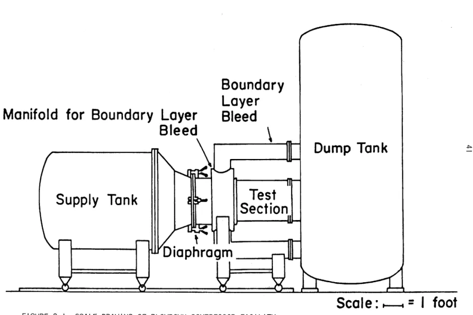
The MIT Blowdown Compressor Facility (Fig. 2.1) used in these
experiments is fully described in Ref. 4, and a short description of
the facility will be presented here. Basically, the Blowdown Facility
consists of a compressor test section (Fig. 2.2) which is initially
separated from a supply tank by an aluminum diaphragm. The test
section is followed by a dump tank into which the compressor discharges.
Before a test, the rotor is brought up to speed in a vacuum and the
diaphragm is ruptured with plastic explosives allowing the test gases
(mixture of Freon and Argon) to flow through the test section. A
throttle plate downstream of the test section controls the mass flow through the stage. If the supply tank pressure remains high enough to choke the throttle plate, axial Mach number will remain constant. The rotor is driven by its own inertia during the test and will
decelerate as it does work on the fluid. On the other hand, the
temperature and pressure in the supply tank (which is essential ly at stagnation condition), decreases as a result of expansion of the gas
into the dump tank. To ensure a constant inlet tangential Mach number, the change in the supply tank temperature and rotor deceleration must
be governed by the relation
W(t) 2 T (t) W(0) T 1 (0)
in the supply tank.
This can be achieved by proper matching of the rotating assembly inertia with supply tank conditions. For the current experiments, the tank pressure required to maintain steady state conditions was
experimental ly determined to be 0.71 atmospheres. Figure 2.3 shows the
matching between the rotor deceleration {w(t)/w(O)}2 and the change in supply tank temperature TI(t)/T1(0). It shows a rather good fit during the test time, constant rotor inlet velocity triangles are achieved.
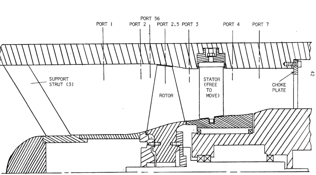
In order to obtain circumferential survey across the stator gaps, a slowly rotating stator (Fig. 2.2) was used with a radially traversed probe. To achieve a slowly rotating stator, a massive hub and tip
rings were attached to the stator blades, so that the rotating stator
wil I have a large moment of inertia. The maximum angular velocity of
the stator is 2% of the rotor angular velocity. Thus during the test,
the stator was allowed to rotate, in the same direction as the rotor, while a probe surveyed downstream of it, moving radially inward. This
setup resulted in a blade-to-blade survey at the same time as the
radial survey.
11.B Test Compressor and Operating Point
The transonic compressor tested is the first-stage of a NASA two
stage fan incorporating low-aspect ratio blading. Details of the
rotor are described in ful I in Ref. 3. The rotor has an aspect ratio
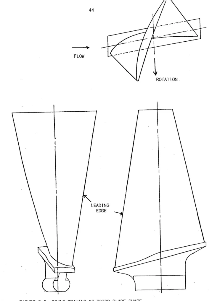
of 1.56, inlet hub-tip ratio of 0.375 and exit hub-tip ratio of 0.478. A drawing of the rotor blade shape is shown in Fig. 2.5. The rotor has 22 blades and the stator has 34 blades. At design speed, the
14
has a total pressure ratio of 1.63.
The stage was tested at 100% design speed in a mixture of Argon and Freon. This corresponds to an initial rotor speed of 201 rps in
the Blowdown experiment, which is about 75% of the design speed when tested in air (267 rps). The operating point of the stage is
deter-mined by the rotational speed of the rotor as well as the throttle
area behind the stage, which controls the mass flow. In the Blowdown experiment this is adjusted by changing the throttle plate (Fig. 2.2).
These two conditions specify the operating point on the performance
map and results can be compared to corresponding data from NASA steady state testing. (Reading number 1283 of Ref. 3.) The average static
radial tip clearances at leading edge were measured to be 0.171 cm
(0.067 in.).
11.C Instrumentation
11.C.1 High Frequency Sphere Probe (Five-Way Probe)
Time resolved measurements of the fluctuating flow field behind
the compressor rotor were determined using a miniature high frequency sphere probe described in Ref. 2. The probe is 0.2 inches in diameter
yielding a frequency response above 30 KHz. It consists of a nearly spherical head on which five silicon pressure sensors are mounted,
(Fig. 2.6 Aand B). The transducer in the center sees nearly stagnation pressure while the two side pairs give good angular sensitivity in two planes. During a compressor test the probe is traversed radially
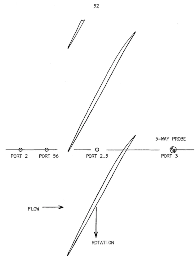
inward with the center transducer perpendicular to the mean flow
direction. This implies that when surveying the flow field behind the rotor (Port 3), it is necessary to turn the probe by a 45* angle
from the center line.
The aerodynamic behavior of the probe has been established by steady state testing of a model twice the size of the actual probe. A set of calibration curves were obtained which cover a range of Mach
numbers from 0.3 to 0.9. The following non-dimensional parameters were retrieved from the calibration measurements and plotted against tangential angle (6) and radial angle ($).
P4 C, (4,M) = P (2.1) 4 T S (A~M) 2 - 3 F3 + W2~ 2 (2.2) C, ($,OM) = I P (2.3) i T Ps P - P H(4,M) = T + (2.4) (3 PI)+ (P 2-Pl) K~ (4OM) 2, 3 S K 2,3( , ,M = 3 1 + (P2~P (2.5)
Some typical calibration curves which correspond to Mach number
0.7 are presented in Fig. 2.8. Since all diaphragms are well upstream
of the separation point on the sphere, Reynolds number effects are weak.
16
from the measured pressures (P I, P2' 3' P4) using an iterative
procedure for which a flow chart is shown in Fig. 2.9. First, assume
a value of Mach number. Values of the static and total pressure,
radial flow angle ($), and pitchwise flow angle (0) can be found from
Equations (2.1) to (2.5). The ratio of total pressure and static
pressure gives a new value for Mach number. If the new Mach number
differs from the guessed value by more than 1%, a new Mach number guess is made and the iteration repeated unti I convergence is achieved.
The probe can travel across the annulus of about 5 inches in
less than 30 milliseconds, which is roughly equal to 15 ft/sec. The
traversing motion of the probe gives rise to a relative radial angle
of -2 degrees. The probe was traversed by pressurizing a piston-type
mechanism while the probe position during the traverse was recorded as a function of test time and is plotted in Fig. 2.7. This figure corresponds to the test in which the probe was put behind the rotor.
The pressure sensitivity of the strain gauged silicon diaphragms may vary between tests and proper calibration is required. This is
done by venting of the facility to atmospheric pressure after each
test. Since the facility pressures are also known at the beginning of a test, these two points can be used to determine the sensitivity for
each individual silicon diaphragm.
All silicon diaphragms used in the sphere probe are highly
temperature sensitive and they experienced thermal drift when used in the Blowdown Tunnel. Besides using resistive compensation circuits, cooling water is used to maintain the probe at a constant temperature.
completely; a compensation scheme is used to correct for thermal drift such that the time averaged total pressure as obtained from the sphere probe agrees with that from a total pressure probe, which is described
in the next section.
ll.C.2 Total Pressure Probe
For measurement of the fluctuating total pressure downstream of the rotor, a probe was designed and constructed with a semi-conducting strain-gauge transducer built directly into the probe head. Figure
2.10 reveals the design details of the probe. The head construction
is very similar to that of usual Pilot probes. The transducer's diaphragm was recessed about one diameter from the entrance in order to make the probe insensitive to variations of the flow direction within 20*. This probe was mounted on a traversing mechanism which allowed the test section radius to be traversed in approximately
30 milliseconds.
The semi-conductor transducer used in the total pressure probe was less sensitive to temperature variations than those on the sphere
probe. It is a Kulite transducer of type XCQ-093 series. Since the
total pressure probe did not have a serious thermal drift problem, the radial variation of total pressure behind the rotor can be obtained by time averaging the signal from the total pressure probe.
11,C.3 Instrumentation Ports
A series of instrumentation ports were located on one side of the test section at the locations shown on Fig. 2.2 and Fig. 2.11.
down-18
stream of the rotor at the tip and is only about 0.2 chords away from
the trailing edge near the hub. Port 4 is at 0.4 chords downstream of the stator. The instrumentation was constructed such that any probe could be used in any port.
11.C.4 Wall Static Measurement and Other Instrumentation
Supply tank and dump tank pressures were measured using pressure transducers which have a lower frequency response and are more stable.
Figure 2.4 shows the change in supply tank pressure, downstream wall static pressure at Port 7 and dump tank pressure during the complete
Blowdown experiment of 600 ms. These flow quantities which have a time constant of variation on the order of one millisecond are referred
to as low speed quantities. A high frequency pressure probe is also put in the casing at about 0.2 chord length (5/8") ahead of the leading
edge of the rotor (Port 56) to give an indication of the shock
strength upstream of the rotor. A simi lar measurement was also taken at mid-chord of the rotor (Port 2.5). This information is particularly
useful in locating the position of the shock. The semi-conductor transducer used in the ti p casing was Kulite strain-gauge transducers
of type XCQ-093 series and was found to be insensitive to temperature changes. The rotor and stator angular positions, radial position of
the 5-way probe and total pressure probe were also monitored during
the test.
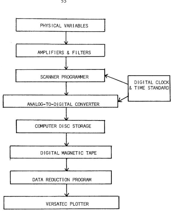
Il.D Data Acquisition and Processing
All signals from various transducers were first amplified. Low speed quantities were then filtered using a low pass analog filter at
I KHz. The signal was then recorded using an on line analog to digital
converter (A/D) having seven high speed channels. Another multiplexed channel is shared by up to 16 low speed measurements. Each high
speed channel has three different sampling rates during a complete
Blowdown test of 600 milliseconds. During the test time the sampling rate is set at 100 KHz, which gives about 25 data points per blade passing. The digitized data was then transmitted to a computer and
stored on the disc. All the data was then backed up onto digital
magnetic tape for permanent storage. A flow chart of data acquisition
20 CHAPTER III
RESULTS
Ill.A Description of Results II.A.I Probe Data Behind Rotor
Wall static measurements at different locations of the test
section are plotted in Figure 2.4 for the complete Blowdown Test of
600 ms. The steady state test time begins at 90 ms and lasts for 30 ms. At about 220 ms the flow velocity is near zero ("slosh point"). As the pressure in the dump tank increases, a point is reached where
pressure in the dump tank equals pressure in the supply tank (Fig. 2.4).
At this point the flow stops and actually reversed its direction. A
typical variation of position of the radially traversing sphere probe
during a test is also shown in Figure 2.7. The initial blade passing
frequency is 4 KHz.
For the remainder of this section, the data will be presented as
functions of dimensionless radius, r/rt, using the actual probe
position for each data set. The probe moves at nearly constant velocity
across the annulus, and since its radial velocity is very small
compared to the rotor or gas velocities, the abscissae may be equally wel I considered proportional to time. Thus each (short) segment of
data may be considered a time history at a given radial position.
The analyzed probe data behind the rotor in absolute (i.e.
non-rotating) coordinates are shown in Figure 3.l.A-C, in which the rotor
total (PT2)TI) and static pressure(PS2 T1 ), and outlet flow angles
are plotted versus radius ratio. Figures 3.1.D-G show the Mach number components computed from the pressures plus the measured flow angles.
Figure 3.1.A shows that there are significant total and static pressure fluctuations in the wakes. Static pressure is by no means
uniform across the wake. The total pressure def lect in the wake is
more pronounced near the hub that at the tip, and the flow is shown to have large blade-to-blade variations. In addition, both pressure
signals show local up-spikes at some radii. The origin of these up-spikes is not fully known yet.
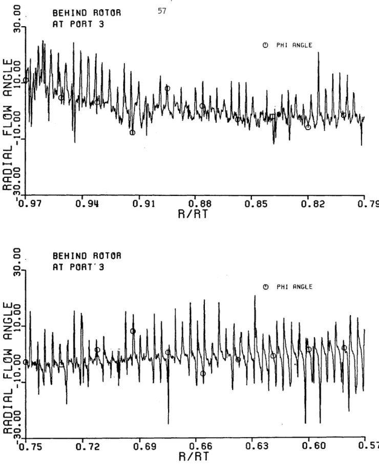
The data presented in Figs 3.1.B and 3.1.C show that there is a large tangential and radial flow angle variation associated with the
wakes. A variation in tangential flow angle in the wake in excess
of 200 have been observed. The variation is relatively periodic from
blade-to-blade for the tangential flow angle. The radial flow angle is defined to be negative if the flow is towards the hub. Figure 3.1.C shows that there is Iarge radial outfIow associated with the wakes, hence they have a highly three-dimensional structure. Rotor wakes at r/rt < 0.63 show a strong negative inf low towards the hub. Variation in radial flow angle of more than -25* have been recorded,
whi ch actually exceeds the range of good probe accuracy. The large inward flows indicated near the hub are thought to be erraneous, due to the close proximity of the spherical probe head to the hub surface. Acceleration of the flow between the probe and the wall would lower
P4, relative to PI, indicating a flow toward the hub.
The calculated Mach number components are shown in Figures
3.l.D-G. Local up-spikes in total Mach number are due to a sudden defect in static pressure shown in Fig. 3.l.A. Axial Mach number is relatively periodic and shows a large defect in the wakes. Figure 3.l.E shows
22
that the wake has an excess of pitchwise Mach number, which is what
one would expect for a rotor wake when observed from a stationary reference frame.
The data as measured from a stationary reference frame can also
be transferred into a rotating reference frame. The results are
presented in this form in Fig. 3.1.H-1, in which the relative flow angle and Mach number are plotted versus radius ratio. Figure 3.1.1
shows that the relative flow Mach number is nearly constant across the passage and drops down in the wakes. We note large variations of wake strength between adjacent blades as inferred from the relative Mach number.
Since the total pressure ratio, exit flow angles and Mach number are measured, we may use Euler's Turbine equation to calculate the
total temperature ratio. However, one must keep in mind that the
equation only applies to a streamtube in which the flow is steady in
a coordinate system relative to the rotor. Although Fig. 3.1.1
(relative Mach number) thus shows that the flow is quite steady, some portions of the flow are unsteady on a blade passing time scale and
substantial error may result in using Euler's equation. It is not
possible with the available data to separate the effects of
blade-to-blade variation in a flow steady in the rotor frame, from unsteadiness
in the rotating frame, as they both appear as a blade-to-blade
variation in the stationary frame.
Introducing convenient non-dimensional variables into Euler's
-rF
2 = + r (-)( ) M I + M 2 2 (3.1)
t0 /YRT t t 2 t0
0
0
Here subscript 0 refers to conditions far upstream in the supply
tank and is assumed to be at the stagnation condition. Figure 3.1.J
shows the computed total temperature ratio; an additional energy input
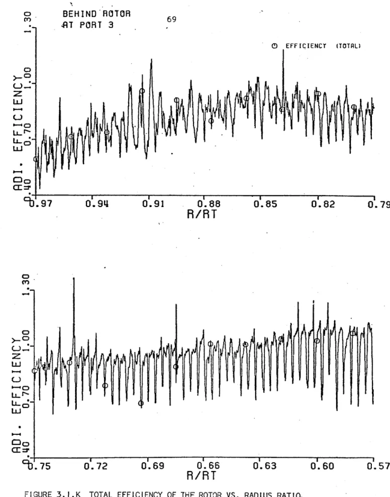
in the wakes is evident. The calculated adiabatic efficiency is plotted in Fig. 3.l.K. It is observed that the local efficiency in
the "inviscid" flow is only about 75% at the tip and is very near
100% for r/rt > 0.8. This is an important source of inefficiency
in transonic rotor and will be further discussed later. It should be noted that the efficiency computation depends mainly on the
stagnation pressure and the peripheral flow angle, which are two nearly independent data from the probe. That the efficiency is so close to unity near the hub is an important consistency check on the probe and
data reduction system. It also adds confidence that the low values
near the tip are meaningful, not due to an error.
Frequency spectrum of all of the above signals are also presented
in Fig. 3.2.A-F.for future reference.
Time averages of several flow variables are illustrated in
Figs. 3.3.A- F together with the design value and measurements taken at NASA Lewis Research Center under steady state conditions (from
Reading No. 1283, Ref. 3). These two sets of data are not strictly
comparable. The MIT data are from a probe traverse just behind the
rotor, as described above. The NASA data on the other hand, are computed
ow
24
behind the stator, the rotor efficiency being taken from such data
in the stator gap. Because of the low aspect ratio of this stage, it would be reasonable to expect a considerable amount of radial
smearing of the rotor outlet profi le. This is in fact very good
agreement for relative flow angle and relative Mach number (Fig. 3.3.E).
Tangential angle and tangential Mach number is also in reasonably good agreement (Fig. 3.3.C). Of considerable importance are the
differences in efficiency near the tip and at midspan shown in Fig. 3.3.A. In the Blowdown test it is observed that there is a region of
low efficiency between r/rt of 0.72 to 0.8, which is manifested as an
increase in total temperature at the same radius. This doesn't appear in the steady state test where the total pressure and total temperature are both measured behind the stator. The local deficiency behind the
rotor may diffuse while passing through the stator. The origin of
this local region of low efficiency may be the shock termination
phenomenon described in Ref. 5. Fluorescence density pictures will
help to reveal the cause of this high loss region.
Efficiency at the tip is also lower in the Blowdown Test. Since
total temperature is about the same at the tip, the difference is due to the total pressure ratio. Streamline curvature program predicts a higher total pressure ratio at the tip, whereas direct measurement
at the Blowdown Tunnel gave a lower reading. This point will be
further examined in Section IlIl.A.3, whre comparison of the data behind the stator is made.
Time averages of Mach number components are presented in Fig. 3.3.D. Results presented in Ref. 3 are data at the trailing edge of
the blade. Since there is an area reduction of about 5% between the
trailing edge of the rotor and at Port 3, static pressure and Mach number can be differed. Acceleration of the flow can lead to a lower static pressure and higher total Mach number at Port 3, as indicated
in Fig. 3.3.B and Fig. 3.3.D. Despite this difference, Mach number components are sti II in reasonably agreement with steady state testing
results.
IIl.A.2 Results of Contour Plots of High Response Data
Anotherway to present the high response data is to construct
contour plots of flow variables in an r-O plane. A continuous time
record of data is broken into segments of 3 blade passing periods long, and the various quantities plotted as functions of peripheral distance
(r0) and radius.
Contour plots of various flow variables in the radial plane 0.5
chords downstream of the rotor are shown in Figs. 3.4.A to 3.4.M. The location of the blade trailing edge is shown on each plot. Because the
blade is highly twisted (see Fig. 2.5) the blade trailing edge wil I not
appear as a vertical line in the r-6 plane. The blade is moving from
right to left and the view corresponds to that of an observer looking
upstream.
It should be emphasized that these data are in a sense taken out
of context since data from several different blades at different times
are combined into a single blade passage. As was previously discussed,
unsteadiness does exist and is important at larger radii. Moreover,
the blades are not identical and blade-to-blade variation may be
26
of detai I in these contour plots is inevitable. Ensemble averaging of the data will suppress the blade-to-blade variation in these
contour plots and flow features common to all blades wiIl be emphasized
by this procedure. Averages over 5 blade passages are presented. A contour plot of the rotor total pressure ratio is shown in Fig. 3.4.A. Between r/rt of 0.90 to 0.70 the flow field can be seen
to have nearly constant total pressure except near the blade wakes. However, there are islands of high total pressure which appear in the
core flow at about r/rt = 0.88. They start from the suction surface
and extend to about mid-passage in the core flow. These islands
of high total pressure are responsible for the localized spots of high efficiency at the same region. No clear explanation can be offered
yet as to the origin of these high total pressure regions. Near the
hub total pressure ratio increases to about 1.72 in the core flow whi le decreasing more in the wakes.
A contour plot of the rotor static pressure ratio (PS2/ TI) is
shown in Fig. 3.4.B. It appears that static pressure ratio is higher
at the blade wake than at the inviscid flow.
The calculated temperature ratio is plotted in Fig. 3.4.C.
Additional energy input in blade wake and in the supersonic flow regions is evident. The rotor adiabatic efficiency is also plotted in Fig. 3.4.D.
Some important conclusions can be drawn from this Figure. At r/rt of
about 0.86, islands of high efficiency occur in the core flow, which
result in a local maximum in the time-averaged efficiency at that
radius (see Fig. 3.3.A). At a little smaller radius (r/r = 0.80), efficiency in the blade wake becomes very low, whereas the core
efficiency rEnains unchanged. The time-averaged efficiency has a
minimum at this radius (see Fig. 3.3.A). Thus the low efficiency that
appears about mid-way between the sonic radius and the tip has its origin from the low efficiency in the blade wake. It is suggested
that a shock termination phenomenon described in Ref. 5 produces strong boundary layer interaction, and resulting in the region of very low
efficiency. Near the tip the efficiency is rather uniform in 0 and in general low, both in the core flow and in the wake. No island of
low efficiency is observed at the tip. If the tip clearance effect were the major source of low tip efficiency, it would seem that the
high velocity jet that escapes from the pressure side to the suction
side should create regions of low efficiency in the core flow due to
mixing loss. No evidence of such low efficiency islands is observed,
although the fact that the measuring plane is about 0.5 chords down-stream may have some effect on this observation.
Contour maps of total Mach number, axial Mach number, pitchwise
Mach number and radial Mach number are included in Fig. 3.4.E through
3.4.H. Since the radial and tangential components of the Mach number on an r-0 plane are shown, we can calculate the vorticity component
perpendicular to the r-0 plane in cylindrical coordinates.
W = V X V
V
aV
av
z r Dr ra6
28
rtz Nb AM0 AM
a r/r Ar/r, ~ rr A
The result is presented in Fig. 3.4.1. Notice a region of strong
streamwise vorticity exists at the trailing edge near the sonic radius. This seems to agree with the model described in Ref. 5. It is argued
that the sharp pressure gradient produced by the shock termination phenomenon would lead to strong radial flows in the boundary layer,
which is unable to withstand the pressure gradients produced in the transonic inviscid flow. The consequent shear would appear in the
form of a streamwise vortex.
Final ly, contour maps of tangential flow angle, radial flow angle,
relative Mach number and relative flow angle are included as Fig. 3.4.J through 3.4.M for future reference. The large disturbances concentrated
at blade passing frequency are clearly displayed in the relative Mach number and tangential angle contour plots (Figs. 3.4.1 and 3.4.J). Also approximate location of blade trailing edge can easily be seen.
ItII.A.3 Results of Probe Survey Behind Stator
The 5-way probe was also traversed across the annulus behind the
stator at Port 4. Time averaged total pressure ratio is i I lustrated in Fig. 3.5, together with the design value and steady state test result from NASA Lewis Research Center. Excellent agreement was
observed in total pressure between the two tests. In all cases, total pressure ratio is decreasing towards the hub, due to increasing stator
and MIT Blowdown test for the rotor, total pressure behind the stator was actually measured directly and no streamline curvature program is involved. Thus at the station where measurements were actual ly taken for both 'tests, results are in good agreement. However, when the total pressure ratio was back calculated using a streamline curvature
program to the station behind the rotor, a discrepancy was found. The directly measured total pressure ratio from the Blowdown Tunnel was about 6-7% lower than that calculated from NASA result at the tip. This
leads to a lower efficiency at the tip for the rotor. It is difficult
to determine which answer is correct. But aside from blockage effects, the direct measurement should be more accurate than using streamline curvature program to calculate the flow field behind the rotor.
A comparison for the time averaged total Mach number behind the
stator is presented in Fig. 3.6. It is observed that the radial ly
averaged total Mach number measured in the Blowdown Tunnel is in very
good agreement with design and NASA steady state results.
Blade-to-blade variation in the flow field behind the stator are
shown in Fig. 3.7.A through Fig. 3.8.E, in which various flow variables
are plotted against radius ratio. Fig. 3.7.A to Fig. 3.7.E correspond to measurements at a plane which is only 0.4 stator chords downstream
of the stator (Port 4). Figure 3.8.A to 3.8.E are from Port 7, which is about 1.5 stator chords downstream of the stator.
From Fig. 3.7.A, one can clearly see the passage of a stator wake, which appears as a minimum in total pressure and a small maximum in
static pressures. Similar behavior in static pressure is found in the rotor wake, as can be seen from the contour plot of Fig. 3.4.B. Both
30
"inviscid" flow. Because of the close proximity of the probe to the stator trailing edge, the stator wake is narrow and one of the
diaphragms on the probe may reside in the stator wake whereas other diaphragms may still be in the inviscid region for several rotor
passing periods. This insufficient spatial resolution of the probe results in erroneous measurements of the flow angles and pressures, thus give rise to the "spikes" in the wake region for the tangential
and radial angles as wel I as the Mach number components. It is observed that the stator wake is deeper at the hub than at the tip.
This measurement is consistent with the design intent and the measurements taken at NASA Lewis Research Center. In both cases,
stator loss increases towards the hub.
The data in the mid-passage shows the state of the rotor wakes as they are convected out of the stator passage. One interesting
feature is that near the tip, the rotor wakes as indicated by the total pressure, Mach number and radial flow angle sti II exist nearly undiminished in the flow downstream of the stator. However, close to the hub some of the rotor wakes seem to have been fi I led up and are hardly dist.inguishable.
Simi lar data from measurement at about 1.5 stator chords down-stream of the stator (Port 7) are shown in Fig. 3.8.A to 3.8.E. Referring back to Fig. 2.2, there is an area reduction of about 6% between Port 4 and Port 7. Moreover, Port 7 is only at 7.94 cm
(3-1/8") from the throttle orifice. These two effects greatly
accelerate the flow, which gives a higher Mach number and lower static pressure.
31
Comparison between data taken with the probe behind the rotor, 0.4 chords behind the stator and 1.5 stator chords behind the stator at the corresponding radii are presented from Fig. 3.9.A to Fig. 3.9.E.
Here total and static pressure, tangential and radial flow angles and
total Mach number at the corresponding radius (r/rt = 0.77) are
plotted; with data taken out in between the stator gap (core flow). It is found that near the tip, the rotor wakes appear nearly undim-inished in the exit of the stator, and remain so in the annular duct
behind the stator. The stator wakes decay very rapidly so that at a distance of 1.5 stator chords behind they have virtually ceased to
exist.
III .A.4. Results of Wal I Static Measurements
High frequency pressure transducers were mounted in the casing
in locations as shown in Fig. 2.11. Fluctuations of static pressure
on those transducers on a blade-to-blade time scale were presented in
Fig. 3.10 - 3.13. Because of limitations of the data acquisition system, high frequency wall static measurements at different locations
along the test section were taken from more than one test, but with the rotor running at exactly the same conditions.
In Fig. 3.10 all signals from Port 2, Port 56 and Port 2.5 are plotted on the same scale so that a comparison between al I three signals can be made. It is evident from the top two signals that the shock wayes rapidly attenuate as they propagate upstream from the
rotor. The bottom trace shows a strong low pressure region at each
blade, evidently due to a tip vortex.
32
signal from Port 2, which is about 0.4 rotor chords from the leading edge of the rotor. Fig. 3.1l.B is the power spectral density of the same signal.
Figure 3. 12.A is the measurement taken at Port 56, which is at 5/8" upstream from the leading edge of the rotor. An inlet relative Mach number of 1.14 is inferred basing on the ratio of the static pressure across a normal shock. It may seem low when compared to the
design value of 1.38, however we must account for the existence of
the boundary layers on the casing. Moreover, the measurement was
taken 5/8" upstream from the leading edge. Besides, the low shock
need not be normal at the tip, thus the inlet relative Mach number
could well be higher than 1.14. tn Fig. 3.12.B the signal at Port 56 from three successive rotations of the rotor is plotted on the same page. Notice one can identify some blades from their relative
shock strength. If desired, this signal can be used as a measure of the rotational speed of the rotor. The small upspike between each blade passing has an unknown origin. The power spectral density of this signal is plotted in Fig. 3.12.C.
The final wall static measurement was taken at Port 2.5, which
is at about mid-chord in the rotor passage. Figure 3. 13.A shows the blade-to-blade variation of this signal. The sharp decrease in static
pressure may be due to the tip vortex associated with each blade.
Notice the magnitude varies slightly from blade-to-blade. This may be due to the variation of tip clearance from one blade to another. Theoretically this signal can be used to predict the location of the
passage shock. However, the highly unsteady nature of the flow made this almost impossible. In Fig. 3.3.1B, data from three successive
rotations of the rotor are plotted on the same page. Notice how the
pressure f iel d between any two b l ades changes from one rotat ion to another. Also there is a large variation from blade-to-blade. This variation strongly suggests an unsteady shock pattern. An unstable oscillating shock system may exist in the passage, which gives rise to the large fluctuation in the inviscid flow from blade-to-blade. Figure 3.13.C is a comparison between the original signals and a
5-cycle ensemble average of the same signals.
Due to relative motion of this moving shock, the rotor shocks
may see a higher approaching Mach number than they would if the
shocks were stationary. Increasing Mach number can increase
shock Iosses significantly, thus giving rise to a lower efficiency in the inviscid core flow. It is still unclear at this point whether the unsteady flow. is an intrinsic feature of transonic compressors, or whether it is due to fluctuations in the quasi-steady flow generated
in the Blowdown Tunnel.
Ill.B. Discussion of Results
Il.B.l Mass Flow Determination and Mach Number Measurements Based on the rate of change of supply tank pressure, the
corrected mass flow of the rotor with respect to air is calculated to be 33.0 Kg/s, This agrees very well with the design value of
33.248 Kg/s. The rate of change of supply tank pressure was, determined
by curve fitting an exponentially decaying function to the original
measured ,supply tank pressure. This avoided differentiating the
34
method, corrected mass flow changed by less than 1% during the test time.
By traversing the 5-way probe upstream of the rotor at Port 1,
it was found that the inlet static pressure is not uniform across the annulus, being lower near the hub. Measurements from the total
pressure probe at different radii showed that the inlet total pressure
is uniform. Thus the non-uniformity in static pressure wil I give a variation in inlet Mach number along the radius. This implies the
rotor is pumping harder near the hub, thus drawing more fluid and hence higher Mach number. According to Ref. 4, mass flow can also be
determined by wall static pressure measurements if the flow is
one-dimensional. However, since static pressure is not uniform across the
annulus, mass flow determination based on casing static pressure
measurement either.upstream or downstream could give misleading results.
Mass flow can also be calculated from the integration of the
flow quantities measured by the 5-way probe along the radius. However,
the accuracy of determining mass flow by this method relies strongly
on the Mach number measured, which is also a function of the static pressure. Since the calibration for static pressure strongly depends
on the geometry of the probe, a slight difference between the model probe used for calibration and the actual probe can lead to a large
error. It was decided to calibrate the actual probe by shifting the
calibration curve for static pressure (K 2,3) such that it gives the
same mass flow as determined by the rate of change of supply tank
pressure. ..Based on this method, the corrected mass flow was determined
(behind stator).
An important consistancy check on the 5-way probe and the data reduction program is in the torque balance calculation on the rotor.
The torque acting on the rotor should balance with the changes in the fluid's angular momentum. The torque acting on the rotor calculated from the rate at which the rotor slows down as it does work on the
fluid during the test time is 303.0 N-m (223.5 lb-ft) and from the change in the angular momentum across the rotor the torque is
calculated to be 301.1 N-m (222.1 lb-ft). The close agreement of the two numbers adds confidence to the data measured by the 5-way
p robe.
Ill.B.2 Rotor Overall Performance
The efficiency of the rotor can be calculated from the rotor
deceleration and mass flow. The moment of inertia of all rotating
parts was determined by a torsional pendulum technique to be 0.293 Kg-m2
(0.216 lb-ft-sec 2). Rotor deceleration was measured by a one pulse-per-revolution tachometer. Using
i C ATT
T
T
IWdt
where i = actual mass f low, Cp = gas constant for Ar-Fe, I = moment of inertia of rotor, w = angular speed, dw/dt = angular acceleration. The overall temperature ratio across the rotor was determined to be
1.174. From the total pressure probe, the rotor time-averaged total
pressure ratio was measured to be 1.677. Thus giving an average
total-to-total isentropic efficiency of 89.5%. This agrees very well
36
a rotor peak adiabatic efficiency of 90.6%.
Although the time-resolved efficiency can be calculated by
using Euler's equation, this method involves several approximations.
Eq. (3.1) was reproduced here.
Tt r r M T 2 + t r I +Y-12-.
t
2 - r + (y-l)(-) jI 2 2 (3.1) YRTt 0 220 0Careful examination of this equation reveals that M2 has a second order effect on the total temperature ratio calculated. However, both
M and r/rt have a strong influence on the calculated total temperature ratio. The probe position (r/rt) can be measured accurately during
the experiment. However, the tangential Mach number, which depends on the total Mach number and tangential flow angle, can hardly be
measured with an accuracy better than 3-5%. One reason is that the
thermal drift problem can offset the D-C level of the total Mach number. More importantly, the tangential flow angle measured depends
on the aerodynamics center of the sphere probe, which may differ from the geometrical center by one or two degrees due to asymmetry. It was
found that the efficiency calculated using Eq. (3.1) is very sensitive to the tangential angle. One degree in tangential flow angle
corresponds to almost 1% in efficiency. The level of the time averaged efficiency plot showed in Fig. 3.3.A was adjusted by varying the
effective probe angle so as to give an overall efficiency of about 90%, as determined from rotor deceleration and mass flow calculation.
Other than the uncertainty in measurements of tangential Mach
number, the application of Euler's equation to the highly unsteady flow is also questionable. In particular, for the portion of flow which
has undergone extensive viscous interaction; such as the hub and tip
casing boundary layers and the blade wakes; the Euler's equation could
be substantially in error, and this should be kept in mind when interpreting the results. Islands of efficiency higher than 100% in Fig. 3.4.D could be due to the above mentioned effects.
When interpreting probe data near the tip, we must also account for the influence of the outer casing on the probe measurement. Close
to the casing the probe wil I no longer act as attached to a thin stem,
but would rather appear as attached to a big block. Moreover, the flow field created by the cavity from which the probe emerges can also affect the data near the tip to a certain extent.
Ill .B.3 Stage Overall Performance
From the total pressure probe, the stage has an average total
pressure ratio of 1.658. After accounting for the rotation of the
stator, the overall total temperature ratio across the stage was
determined to be 1.181, thus giving an average efficiency of 86.2%. This is based on radially averaging the circumferentially averaged
flow behind the stator, including the stator wakes. The stage
efficiency is calculated by finding the stage total temperature from
the rotor deceleration and then accounting for the sma I I stator
rotation. Corresponding measurements at NASA Lewis Research Center
have given a peak stage efficiency of 87.0%.
A comparison between measurements from the 5-way probe and the
total pressure probe at different radii was presented in Fig. 3.14.A & B . Here the total pressure ratio and the corresponding power spectral
38
are essentially the same in both measurements. The flow is highly
unsteady at a higher radius. At a lower radius, blade wake is more
clearly defined. Similarity in both signals adds confidence to the
measurements taken using the 5-way probe.
One of the more important results of this work is presented in Fig. 3.15. Here the time-averaged efficiency in the inviscid core flow as estimated from Fig. 3.1.K is separated from the efficiency in wake flow. The difference between this core flow efficiency and the overall efficiency is interpreted as a viscous profile loss and
is plotted in Fig. 3.15 as the half filled circles. The sum of these plus shock losses based on normal shocks at the inlet relative Mach number are also plotted, as the triangular points. One observation
is that the overall efficiency is well below the estimate based on the sum of normal shock and profile losses, that is normal shock
losses do not account for the core flow inefficiency. Profile losses are relatively small, accounting for only about 4% of the inefficiency, and are relatively constant along the radius. Near the tip, normal shock losses only account for less than 5% of the inefficiency. As can be seen, there is at least a 5% increment in overall rotor or stage inefficiency not explained by these mechanisms, with a much la-rger discrepancy near the tip. Thus it is important to understand the mechanisms which control the losses in the tip region.
CHAPTER IV CONCLUSIONS
An investigation of the flow field produced by a transonic compressor stage has been completed. This study included time and space resolved flow measurements behind the rotor and stator, as well
as tip casing wal I static pressure measurements. Spatial and temporal resolution achieved by the 5-way probe was sufficient to determine velocity components and pressures inside individual blade wakes and in the surrounding flow. Large variations in both tangential and radial
flow angles in the rotor wakes were observed, showing the highly
three-dimensional structure of rotor wakes which is very different from two-dimensional models. Five-way probe data also showed that
the flow is highly unsteady and has large blade-to-blade variation. Contour plot in an r-e plane indicates a strong streamwise vortex
near the sonic radius, which can represent a region of high losses.
Time and space resolved measurements of flow behind a row of
stator blades downstream.of the transonic rotor show that there is a significant total pressure defect associated with stator wakes. A small maximum in static pressure was also observed in the stator wake. The wakes from the rotor exist nearly undiminished in the exit flow
from the stator and remain so in the annular duct behind the stator. The stator wakes decay very rapidly so that at a distance of 1.5 stator
chords behind the stator they have virtually ceased to exist.
Wal I static measurements from high frequency wal I static trans-ducers at mid-chord of the rotor strongly suggests a highly unsteady
40
relative Mach numbers which could increase shock losses significantly.
Though sufficient evidence cannot be obtained in the Blowdown Tunnel to confirm this observation, this unstable oscillating shock system can represent an important source of losses and deserve further
investigation.
Although the 5-way probe has excellent frequency response, it is limited by its relative large size. Besides the blockage effects, the probe also larks sufficient spatial resolution to resolve data
inside the rotor wakes. These problems can be lessened somewhat if the present probe can be reduced in size by a factor of two.
The viability of the Blowdown Compressor and its associated instrumentation for providing the required experimental data has been fully demonstrated. However, developing a technique to measure total temperature becomes very desirable for this facility. As reported, determining efficiency based on Euler's equation is by no means
accurate. Only with a very precise measurement of total temperture can the performance of the rotor be ful ly evaluated. Since efficiency
is the most sensitive indicator of the quality of the aerodyanmic design of the compressor, it is important to develop a technique to
measure the total temperature.
Manifold for Boundary Layer
Bleed
Dump Tank
Supply Tank
Diaphragm
Boundary
Layer
Bleed
Sca
le: -
I
foot
FIGURE 2.1 SCALE DRAWING OF BLOWDOWN COMPRESSOR FACILITY.
I
INSTRUMENTATION PORTS
PORT I
PORT 56
PORT 2 PORT 2.5 PORT 3 PORT 4 PORT 7
SUPPORT SAO
RU (3) AR CHOKE
TO PLATE
ROTOR VE)
Cc 0 -L -o
cu
-20.00
TIME
3M.S
)
(M3)
.7 0 Uy) 0 00 Ln 0) 0l60.00
x 10
O SUPPLY TANK A DOWNSTRERM; PORT + DUMP TANK TEST TIMEODEL ROTOR SPEED SQ.
A
SUPPLY TNK TEMPRATI T (t) T (0) 2-U
90.00
TIME
TEST TIME110.00
(MS)
I130.00FIGURE 2.4 PRESSURE VARIATION IN BLOWDOWN FACILITY AT DIFFERENT LOCATIONS
FIGURE 2.3 MATCHING BETWEEN ROTOR DECELERATION AND CHANGE IN SUPPLY TANK TEMPERATURE 070.00 0) 0
10.00
'.0010.00
50.0044
FLOW
ROTATION
LEADING EDGE
45 3> .o 0 Ln 1) .c
I-0
0
0 45 0. 20" 4I 5 El 0 0 0 0) 0 0a
0a:c;
0 0 0 CD 0FIGURE 2.6.B SKETCH OF 5-WAY PROBE SHOWING AIR ANGLE DEFINITION.
5-WRY PROBE POSITION BEHIND ROTOR
o.oo 1'o.oo '10.00 120.00 130.00
TIME (MS)
FIGURE 2.7 5-WAY PROBE POSIT40N VS. TIME DURING THE TRAVERSE (PROBE BEHIND ROTOR)