HAL Id: hal-02265770
https://hal.archives-ouvertes.fr/hal-02265770
Submitted on 4 Nov 2020
HAL is a multi-disciplinary open access
archive for the deposit and dissemination of
sci-entific research documents, whether they are
pub-lished or not. The documents may come from
teaching and research institutions in France or
abroad, or from public or private research centers.
L’archive ouverte pluridisciplinaire HAL, est
destinée au dépôt et à la diffusion de documents
scientifiques de niveau recherche, publiés ou non,
émanant des établissements d’enseignement et de
recherche français ou étrangers, des laboratoires
publics ou privés.
Relative magnetic helicity as a diagnostic of solar
eruptivity
E. Pariat, E. Leake, G. Valori, G. Linton, F. Zuccarello, K. Dalmasse
To cite this version:
E. Pariat, E. Leake, G. Valori, G. Linton, F. Zuccarello, et al.. Relative magnetic helicity as a
diagnostic of solar eruptivity. Astronomy and Astrophysics - A&A, EDP Sciences, 2017, 601, pp.A125.
�10.1051/0004-6361/201630043�. �hal-02265770�
DOI:10.1051/0004-6361/201630043 c ESO 2017
Astronomy
&
Astrophysics
Relative magnetic helicity as a diagnostic of solar eruptivity
E. Pariat
1, J. E. Leake
2, 6, G. Valori
3, M. G. Linton
2, F. P. Zuccarello
4, and K. Dalmasse
51 LESIA, Observatoire de Paris, PSL Research University, CNRS, Sorbonne Universités, UPMC Univ. Paris 06, Univ. Paris Diderot,
Sorbonne Paris Cité, 92195 Meudon, France e-mail: [email protected]
2 Naval Research Laboratory, Washington, DC 20375, USA
3 UCL-Mullard Space Science Laboratory, Holmbury St. Mary, Dorking, Surrey, RH5 6NT, UK
4 Centre for mathematical Plasma Astrophysics, Department of Mathematics, KU Leuven, 3001 Leuven, Belgium 5 CISL/HAO, National Center for Atmospheric Research, PO Box 3000, Boulder, CO 80307-3000, USA 6 Now at: NASA Goddard Space Flight Center, Greenbelt, MD 20711, USA
Received 10 November 2016/ Accepted 27 March 2017
ABSTRACT
Context.The discovery of clear criteria that can deterministically describe the eruptive state of a solar active region would lead to major improvements on space weather predictions.
Aims.Using series of numerical simulations of the emergence of a magnetic flux rope in a magnetized coronal, leading either to eruptions or to stable configurations, we test several global scalar quantities for the ability to discriminate between the eruptive and the non-eruptive simulations.
Methods.From the magnetic field generated by the three-dimensional magnetohydrodynamical simulations, we compute and analyze the evolution of the magnetic flux, of the magnetic energy and its decomposition into potential and free energies, and of the relative magnetic helicity and its decomposition.
Results. Unlike the magnetic flux and magnetic energies, magnetic helicities are able to markedly distinguish the eruptive from the non-eruptive simulations. We find that the ratio of the magnetic helicity of the current-carrying magnetic field to the total relative helicity presents the highest values for the eruptive simulations, in the pre-eruptive phase only. We observe that the eruptive simulations do not possess the highest value of total magnetic helicity.
Conclusions.In the framework of our numerical study, the magnetic energies and the total relative helicity do not correspond to good eruptivity proxies. Our study highlights that the ratio of magnetic helicities diagnoses very clearly the eruptive potential of our parametric simulations. Our study shows that magnetic-helicity-based quantities may be very efficient for the prediction of solar eruptions.
Key words. magnetic fields – magnetohydrodynamics (MHD) – plasmas – Sun: activity – Sun: flares – Sun: coronal mass ejections (CMEs)
1. Introduction
The reliable prediction of the triggering of solar eruptions is an essential step toward improving space weather forecasts. How-ever, since the underlying mechanisms leading to the generation of solar eruptions have not yet been indisputably determined, no sufficient conditions of solar eruptivity have yet been es-tablished. Solar flare predictions are thus still strongly driven by empirical methods (e.g.,Yu et al. 2010;Falconer et al. 2011,
2014; Barnes et al. 2016). Nowadays most predictions rely on the determination and characterization of solar active regions through the use of several parameters and the statistical compari-son with the historical eruptivity of past active regions presenting similar values of these parameters. This empirical methodology has driven the quest for the determination of which parameter, or combination of parameters, would be the best proxy of the erup-tivity of solar active regions. Multiple studies have thus analyzed a relatively vast list of quantities, extracting them from existing observations of active regions and comparing them with the ob-served eruptivity (e.g.,Leka & Barnes 2003a,b,2007;Schrijver 2007;Bobra & Couvidat 2015;Bobra & Ilonidis 2016). No sim-ple singular parameter has yet been found to be a reliable proxy of solar eruptivity. Thanks to advances in computer science, with
the development of data-mining methods and machine-learning algorithms, this search and its direct application to new flare pre-diction systems are now reaching a new stage of development with projects such as FLARECAST1.
The determination of pertinent parameters of eruptivity has so far been almost exclusively based on observational data. De-spite tremendous advances in numerical modeling of solar erup-tions, few studies have used numerical simulations to advance the search for eruptivity criteria. This is partly due to the fact that numerical models are strongly driven by either having a high level of realism (Lukin & Linton 2011; Baumann et al. 2013;
Pinto et al. 2016;Carlsson et al. 2016) or focus on case-by-case studies of observed events (Jiang et al. 2012;Inoue et al. 2014;
Rubio da Costa et al. 2016). Little effort is spent on perform-ing systematic parametric simulations which would allow the determination of eruptivity criteria. Similarly to observations, the search for proxies of eruptivity requires models which are parametrically able to produce both eruptive and non-eruptive simulations. Kusano et al. (2012) presents one of the few ex-amples of such a simulation setup. By varying two parameters,
Kusano et al.(2012) has been able to derive an eruptivity matrix based on the relative orientation of two magnetic structures.
Recently, Leake et al. (2013) and Leake et al. (2014) pre-sented three-dimensional (3D) magnetohydrodynamical (MHD) simulations of magnetic flux emergence into a stratified atmo-sphere with a pre-existing background coronal magnetic field. Depending on the relative orientation of, and hence the amount of reconnection between, the emerging and pre-existing mag-netic flux systems, both stable and eruptive configurations were found. There have been many other studies of magnetic flux emergence, with similar parameters for the emerging flux sys-tem as those inLeake et al.(2013) andLeake et al.(2014), and a review of some of them can be found in Cheung & Isobe
(2014). In general, eruptive behavior requires some reconnec-tion between emerging and pre-existing flux systems, but some previous studies also exhibit eruptive behavior without the ex-istence of a coronal field and this external reconnection (e.g.,
Manchester IV et al. 2004).
Along with Guennou et al. (in prep.), the present study is dedicated to the analysis of the eruptivity properties of the sim-ulations ofLeake et al. (2013,2014). Our goal is to determine whether or not a unique scalar quantity, computable at a given instant, is able to properly describe the eruptive potential of the system. While Guennou et al. (in prep.) is focusing on the analy-sis of quantities than can be derived solely from the photospheric magnetic field, similarly to what is done with real observational data, the present work will be restricted to a few quantities com-puted from the coronal volume of the system.
Magnetic energy and magnetic helicity are typical scalar quantities that contribute to the description of a 3D magnetic system at any instant. Magnetic energy is known to be the key source of energy that fuels solar eruptions. However, only the so-called free magnetic energy (or non-potential energy), the frac-tion of the total magnetic energy corresponding to the current-carrying part of the magnetic field, can actually be converted to other forms of energy during a solar eruption (e.g.,Emslie et al. 2012;Aschwanden et al. 2014). The non-potential energy of an active region has actually been observationally found to be pos-itively correlated with the active region’s flare index and erup-tivity; it does not, however, provide by itself a necessary crite-rion for eruptivity (Schrijver et al. 2005;Jing et al. 2009,2010;
Tziotziou et al. 2012;Yang et al. 2012;Su et al. 2014).
Magnetic helicity is a signed scalar quantity that quanti-fies the geometrical properties of a magnetic system in terms of twist and entanglement of the magnetic field lines. Mag-netic helicity, together with magMag-netic energy and cross helic-ity, are the only three known conserved quantities of ideal MHD. Differently from the other two, however, magnetic he-licity has the property of being quasi-conserved even when in-tense non-ideal effects are developing (Berger 1984;Pariat et al. 2015). Magnetic helicity conservation has been suggested to be the reason behind the existence of ejection of twisted magne-tized structures, that is, coronal mass ejections (CMEs), by the Sun (Rust 1994; Low 1996). There is observational evidence that magnetic helicity tends to be higher in flare-productive and CME-productive active regions compared to less productive active regions (Nindos & Andrews 2004; LaBonte et al. 2007;
Park et al. 2008, 2010; Tziotziou et al. 2012). Magnetic helic-ity conservation can also be used to predict the outcome of different magnetic interactions, for example, tunnel reconnec-tion (Linton & Antiochos 2005). Magnetic helicity evolution has already been studied in several flux-emergence simulations (e.g., Cheung et al. 2005; Magara 2008; Moraitis et al. 2014;
Sturrock et al. 2015;Sturrock & Hood 2016) but without any fo-cus on the possible link between helicity and eruptivity.
The goal of the present study is thus to determine whether or not quantities based on either magnetic energy or magnetic helicity are able to describe the eruptivity potential of the para-metric flux emergence simulations of Leake et al. (2013) and
Leake et al. (2014), which are described in Sect.2. In Sect.3
we present the magnetic-flux and the magnetic-energy time evo-lutions in the different simulations. Section4analyses and com-pares the magnetic helicity properties of the different parametric cases. In Sect.5, we compare the different proxies of eruptivity. We obtain the very promising results that the ratio of the current-carrying magnetic helicity to the total magnetic helicity consti-tutes a very clear criterion describing the eruptive potential of the simulations. In Sect.6, we finally discuss the limitations of the present analysis and the possible application of the eruptivity criterion highlighted in this study.
2. Eruptive and non-eruptive parametric flux emergence simulations
The datasets analyzed in this study are based on the 3D visco-resistive MHD simulations presented inLeake et al.(2013, here-after L13) andLeake et al.(2014, hereafter L14). L13 and L14 have performed and analyzed simulations of the emergence of a twisted magnetic flux rope in a stratified solar atmosphere. The flux tube, initially located in the high-density bottom part of the simulation box (assumed to emulate the convection zone), is made buoyant and rises up in the high-temperature corona go-ing through a minimum temperature region emulatgo-ing the solar photosphere. In all seven simulations considered here, the initial conditions constituting the emerging flux rope and the thermody-namical properties of the atmosphere are kept strictly constant. The atmospheric stratification and the initial condition of the flux rope are typical of emergence simulations, and are presented in detail in L13 and L14. The simulations are also performed with the very same numerical treatment. The employed mesh is a 3D irregular Cartesian grid with z corresponding to the vertical di-rection (the gravity didi-rection), y the initial didi-rection of the axis of the emerging flux rope, and x the third orthonormal direction. The boundary conditions are kept similar for the seven paramet-ric simulations for which the system is evolved with the same Lagrangian-remap code Lare3D (Arber et al. 2001). The numer-ical method is also presented in detail in L13 and L14. The sim-ulations are performed in non-dimensional units; scaling that we are keeping in the present study. An example of a physical scal-ing is presented in L13 and L14. Another choice of scalscal-ing is introduced in Guennou et al. (in prep.).
The seven simulations differ by the properties of the initial (t = 0) background field that represents the pre-existing coro-nal field. In these simulations an arcade magnetic field is chosen which is invariant along the y-direction, that is, parallel to the axis of the flux tube at t= 0. The magnetic field is given by
BArc = ∇ × AArc, where, (1)
AArc = Bd(0,
z − zd
(x2+ (z − z d)2)3/2
, 0), (2)
with zd the depth at which the source of the arcade is located
and Bda signed quantity controlling the orientation (the sign of
Bd) and the magnetic strength (|Bd|) of the arcade. This
mag-netic field has an asymptotic decay of 1/z3. The arcade is
ini-tially perpendicular to the convection-zone flux tube’s axis, and thus is aligned along the same axis as the twist component of
Table 1. Parametric simulations.
Label No Erupt SD No Erupt MD No Erupt WD No Erupt ND Erupt WD Erupt MD Erupt SD
Bd 10 7.5 5 0 −5 −7.5 −10
Arcade strength Strong Medium Weak Null Weak Medium Strong
Eruption No No No No Yes Yes Yes
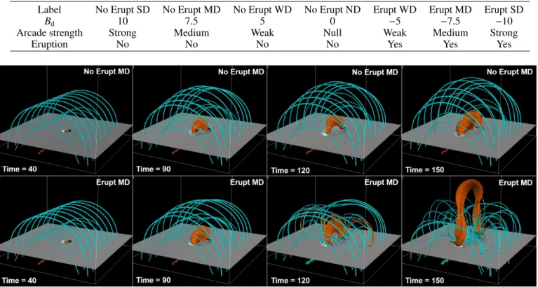
Fig. 1.Snapshots comparing the evolution of the systems in the eruptive (bottom row) and non-eruptive (top row) cases with medium arcade strength (Bd = ±7.5). The respectively (cyan, orange) field lines initially belong to the (arcade, emerging flux rope). The two-dimensional (2D)
horizontal cut displays the distribution at z= 0 of the vertical component of the magnetic field, Bz with a gray-scale code. Only the volume above that boundary is considered in the present study.
the flux tube’s magnetic field. The seven parametric simulations presented in this paper correspond to seven different values of Bdgiven in Table1. The simulations with a positive Bd, which
led to a stable configuration, have been presented in L13 while the simulations with a negative Bd, which induced an eruption,
were presented in L14. The magnetic arcade strength |Bd| has
four different normalized values, that is, [0, 5, 7.5, 10], which respectively correspond to configurations with no arcade (ND), a weak arcade (WD), a medium arcade (MD), and a strong ar-cade (SD), following the notation of L13 and L14.
The simulation with Bd = 0 corresponds to the absence of
coronal magnetic field. This simulation was presented both in L13 and L14 and used as a idealized reference simulation. In the real solar corona some small magnetic field is always present. L13 and L14 showed that the emergence of the flux rope in the magnetic-field-empty corona led to the formation of a sta-ble magnetic structure in the solar corona. No eruptive behavior was observed. In the present manuscript this simulation is la-beled “No Erupt ND”.
The three simulations with Bd > 0 were presented in L13.
For this configuration the direction of the arcade field is par-allel to the direction of the upper part of the poloidal field of the twisted emerging flux rope. Figure 1, top panels, presents the typical evolution of the system in the Bd = 7.5 case. In this
setup, the flux rope emerges into a field in a configuration which is unfavorable for magnetic reconnection. As the initial flux rope emerges, these simulations result in the formation of a new stable coronal flux rope. The flux rope, as with the no-arcade configu-ration, does not present any eruptive behavior and remains in the coronal domain until the end of the simulations. Hereafter, these three simulations are labeled “No Erupt WD”, “No Erupt MD”,
and “No Erupt SD” according to the strength of the magnetic arcade (respectively with Bd= [5, 7.5, 10]).
The three simulations with Bd < 0 were presented in L14.
Fig.1, bottom panel, displays the typical evolution of the sys-tem for the Bd = −7.5 simulation. For this configuration, the
direction of the arcade field is antiparallel to the direction of the top of the twisted emerging flux rope. In this setup, the flux rope emerges into a coronal field for which the orientation is favorable for magnetic reconnection. Similarly to the non-eruptive simu-lations, the emergence results in the formation of a new coro-nal flux rope. However, in contrast to the Bd ≥ 0 cases, here
the new coronal flux rope is unstable and erupts. The secondary flux rope is immediately rising upward exponentially in time and eventually ejected up from the simulation domain. Once the ejection occurs, the remaining coronal magnetic field remains stable with no further eruption, even though residual flux emer-gence was still underway. In the following, these three simula-tions are labeled “Erupt WD”, “Erupt MD”, and “Erupt SD” ac-cording to the strength of the magnetic arcade (respectively with Bd = −[5, 7.5, 10]).
Since observational studies are not yet able to provide in-formation about the sub-photospheric magnetic field, we only focus on analyzing the atmospheric part of the flux emergence simulations of L13 and L14. The datasets analyzed here thus correspond to the following subdomain: x ∈ [−100, 100], y ∈ [−100, 100], z ∈ [0.36, 150]. To comply with the constraints of our magnetic helicity estimation routines, the original irregular 3D grid of L13 and L14 is remapped on a 3D regular and uni-form mesh, using trilinear interpolation. The grid used in the present study has a constant pixel size of 0.859 along all three dimensions. This corresponds to [1.3, 2], respectively, times the
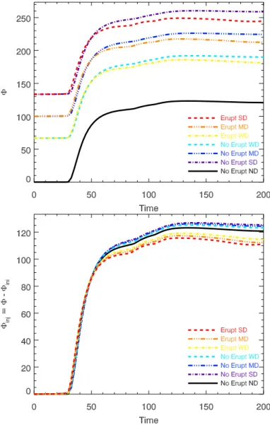
Fig. 2.Evolution of the absolute magnetic flux (Φ, top panel) and of
the injected magnetic flux (Φinj ≡Φ − Φ(t = 0), bottom panel) in the
system for the 7 parametric simulations. The non-eruptive simulation without surrounding field (No Erupt ND) is plotted with a continu-ous black line. The non-eruptive simulations with respectively (strong, medium, weak) arcade strength, labelled (No Erupt SD, No Erupt MD, No Erupt WD), are plotted respectively with a (purple dot dashed, blue dot-dot-dot-dashed, cyan dashed) line. The eruptive simulations with respectively (strong, medium, weak) arcade strength, labelled respec-tively (Erupt SD, Erupt MD, Erupt WD), are plotted respecrespec-tively with a (red dashed, orange dot-dot-dot-dashed, yellow dot dashed) line.
smallest horizontal and vertical grid spacing used in the original simulations in L13 and L14, located at the center of the simula-tion, and [0.33, 0.43] times its largest grid spacing, respectively. As discussed in Sect.4.1, this interpolation deteriorates the level of solenoidality (∇ · B = 0) of the magnetic field compared to the original data of L13 and L14.
The simulations last from t = 0 to t = 200. For all the simulations, before t ∼ 30, the emerging flux rope rises in the convection zone, and the coronal field (that is, the domain stud-ied here), remains close to its initial stage. The rising flux ropes eventually reach the photospheric level, and in our datasets the emergence effectively starts around t ∼ 30 (see Fig. 2). In the eruptive simulations, as soon as the flux tube starts to rise in the corona, a current sheet builds up above the emerging flux rope at the boundary with the antiparallel coronal magnetic field. This
induces continuous mild magnetic reconnection (referred to as “external” reconnection in Sect. 3.1 of L14) between the emerg-ing flux rope and the overlyemerg-ing coronal field . This reconnec-tion is weaker than the “internal” reconnecreconnec-tion observed from t ∼120 low in the corona, within this emerging flux rope, only in the eruptive simulations of L14, Sect. 3.3, where reconnection within the emerging flux structure is temporally coincident with an eruption. The external reconnection is qualitatively character-ized as “mild” relative to the internal reconnection with regards to the relative intensity of the current sheets of the reconnection flows and of the overall dynamics of the magnetic flux processed. In the following, the period t ∈ [30, 120] will be referred to as the pre-eruptive phase both for the eruptive and the non-eruptive simulations. An efficient proxy of eruptivity should be able to distinguish the eruptive- from the non-eruptive simulations dur-ing the pre-eruptive phase only.
Intense magnetic reconnection around the flux rope enables its ejection in the eruptive simulation. The flux rope eventually crosses the top boundary of our dataset (at z = 150) around t ∼ 150. The period between t ∼ 120 and t ∼ 150 is named hereafter as the eruptive phase. The period with t > 150, until the final time analyzed in this study at t= 200, is the post-eruptive phase. It should also be noted that the non-eruptive simulations have been carried out until t > 450. No eruptive behavior was sighted in that later phase of their evolution. At the end of the time range studied here, the non-eruptive simulations are thus still not in an eruptive stage. Hence during the post-eruptive phase, since both the non-eruptive and the eruptive simulations are in a stable state, an efficient eruptivity proxy should not be able to discriminate between them, in addition to being able to discriminate between them in the pre-eruptive phase.
3. Magnetic flux and energy evolution
Before analyzing the differences in the magnetic helicity content in the simulations, it is important to first compare the evolution of the magnetic flux and magnetic energies, quantities which are typically used to characterize eruptive systems such as active re-gions. More frequent and powerful CMEs are known to origi-nate from active regions with higher magnetic flux. As discussed in Sect.1, they are theoretically expected and observationally found to have a relatively high non-potential energy, and hence have a greater reserve of energy to fuel the eruption.
3.1. Magnetic flux
The magnetic fluxΦ, half the total unsigned flux, at the bottom boundary of the system is given by:
Φ =1
2 Z
z=0
|B · dS| . (3)
Its evolution in time for the seven different simulations is rep-resented in the top panel of Fig. 2. Because of the different values of the strength of the arcade, the initial magnetic flux Φini≡Φ(t = 0) in the seven simulations has different intensities.
While the simulation with no arcade possesses no initial mag-netic flux, the amount ofΦini in the other simulations is simply
related to the arcade strength. As theoretically expected, one has
Φini,MD/Φini,WD = 3/2 and Φini,SD/Φini,MD = 4/3. In the present
simulation framework, it is obvious that the magnetic flux does not constitute a discriminative factor for eruptivity. The values of Φ for the eruptive and non-eruptive simulations are completely intertwined.
Because the simulation setup consists of a flux rope emerg-ing into a coronal field, it is interestemerg-ing to plot the injected mag-netic flux, here defined as the flux added to the pre-existing field. In the bottom panel of Fig.2, we represent the injected magnetic flux,Φinj, defined, for each simulation, in reference to its initial
magnetic flux,Φini:
Φinj≡Φ − Φini. (4)
The curves ofΦinj show very strong similarities in terms of
in-jected flux. This is expected since the very same magnetic struc-ture is emerging in all seven runs. For all seven cases, the emer-gence starts around t ∼ 30 and presents a very sharp increase until t ∼ 60. During that period, more than 80% of the magnetic flux is injected in the systems. In this first phase of the emer-gence, the curves are barely distinguishable from one another. The curves only begin to differ slightly after t ∼ 65. This differ-ence is likely due to mild external reconnections occurring in the eruptive simulations as the emerging flux rope interacts with the overlying anti-parallel field, lightly perturbing and reducing the amount of flux emerging compared to the non-eruptive runs.
After that, the magnetic injection increases moderately be-fore reaching a plateau and slightly decreasing. The quantityΦinj
is therefore not able to discriminate the eruptive behavior present in the different simulations. No distinctive signature of eruptivity is present in the curves of the magnetic fluxes in the pre-eruptive phase.
3.2. Magnetic energies
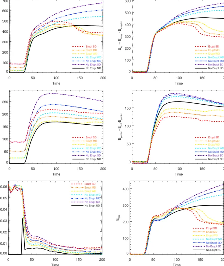
The magnetic energy being the central source of energy in ac-tive solar events motivates us to present in Fig.3, top left panel, the evolution of the magnetic energy Emagfor the different
sim-ulations. Similarly toΦ, because of the difference in the initial magnetic coronal field, Emagdoes not constitute a pertinent
cri-terion of eruptivity. For each simulation, we also plot the in-jected magnetic energy Einj, defined relative to the initial value
Emag,ini≡ Emag(t= 0):
Einj≡ Emag− Emag,ini. (5)
As forΦinj, the evolution of Einjfor the different simulations in
the initial phase of the emergence, between t = 30 and t = 65, presents extremely similar properties. One simulation is barely distinguishable from any other one. In the pre-eruptive phase of the eruptive simulations, the mild external reconnection in-duces a lower magnetic flux injection (cf. Fig.2) that results in a slightly lower injected magnetic energy. It is only once the sys-tem is erupting, for t > 120, that Einjstarts to present significant
differences between the eruptive and non-eruptive cases. This is likely due to the ejection of the erupting current-carrying struc-ture outside of the simulation domain. In any-case, this indicates that Einj, similarly toΦinj, does not represent an efficient
eruptiv-ity criterion that would allow a forecast of the eruptions. As discussed inValori et al.(2013), the magnetic energy of a magnetic field with finite non-solenoidality (∇ · B , 0), can be decomposed as:
Emag= Epot+ Efree+ Ens, (6)
where Epotand Efreeare the energies associated with the potential
and current-carrying solenoidal contributions, respectively, and Ensis the sum of the non-solenoidal contributions (see Eqs. (7),
(8) inValori et al. 2013, for the corresponding expressions). The potential field is computed such as to match the normal compo-nent of the field on all six boundaries. In the case of a purely
solenoidal field, Ens = 0 in accord with the Thompson
theo-rem. However, since numerical datasets never induce a perfectly null divergence of B, a finite value of Ens is generally present.
Unlike other physically meaningful energies, Ens is a
pseudo-energy quantity, which can be positive or negative.
The different values of the decomposition of energy are plot-ted in Fig.3. While the potential energy presented in the middle panel of Fig.3 does not constitute an interesting criterion for eruptivity, its evolution is interesting for understanding the en-ergy accumulation. Initially the system is fully potential, that is, Efree = 0 and Emag(t = 0) = Epot(t = 0). As the flux starts
to emerge, the potential energy increases due to the modifica-tion of B at the six side-boundaries of the domain. While at the very beginning of the emergence, for t ∈ [30, 40], the poten-tial field of the eruptive and non-eruptive simulations shows a similar increase, the non-eruptive simulations possess a signif-icantly higher potential energy compared to the eruptive simu-lation done at equivalent arcade strengths. At t = 80, the non-eruptive simulation of a given |Bd| contains approximately 1.2
times more potential energy than its counterpart eruptive run. This further confirms that the potential energy, and its relative accumulation, cannot constitute a good eruptivity criterion.
We also notice that a large part of the injected magnetic en-ergy, Einj, is comprised of the increase in the potential energy,
although not the majority. Before t ∼ 100, the potential en-ergy represents approximately one third of the accumulated to-tal magnetic energy. This shows, as inPariat et al. (2015), that taking Einj as a proxy for the free magnetic energy Efree, as is
frequently done, can lead to substantial errors, and that prop-erly computing the energy composition of Eq. (6), using the full boundary information, is an important step of any proper energy budget analysis.
The free magnetic energy, Efree, is a fundamental quantity in
solar eruption theory. As the primary energy tank for all the dy-namics of the phenomena developing during a solar eruption, its estimation is a main focus of solar flare studies (Tziotziou et al. 2012,2013;Aschwanden et al. 2014). The bottom right panel of Fig.3presents the time variations of Efreefor the seven
paramet-ric simulations studied here. As forΦinjand Einj, Efree presents
a relatively similar dynamic for the seven simulations in the first half of each simulation. Unlike previous criteria, the curves of Efreefor the eruptive simulations tend to be slightly higher than
for the non-eruptive ones. The additional free magnetic energy remains, however, weakly higher. Interestingly, after t ∼ 100, the values of Efree for the eruptive simulations tend to decrease
and become lower than the ones of the non-eruptive simulations. This behavior confirms the common theoretical understanding that Efree is indeed a quantity tightly linked with the eruptive
dynamics. Nonetheless, the highest values of Efreeachieved are
reached by the non-eruptive simulations in the post eruptive phase. Thus, while Efree certainly represents a necessary
con-dition for flares, it does not seem to be a significant sufficient condition for eruptivity.
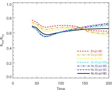
The ratio of the free magnetic energy to the injected magnetic energy, Efree/Einj, is a potentially interesting proxy for
eruptiv-ity. Indeed, as shown in Fig.4, the eruptive simulations are well distinguishable from the non-eruptive ones already in the pre-eruptive phase using this criterion. For t ∈ [0, 40], as the flux rope has not yet emerged, the injected energy is basically zero at the numerical precision. During that period, the plotted ratio is dominated by the variations on the numerical rounding preci-sion in the numerator of the Efree/Einj ratio. We have thus
dis-regarded this part of the evolution in the plot. For t ∈ [40, 130], we note that the eruptive simulations present a higher ratio of
Fig. 3.Energy evolution in the system for the seven parametric simulations: total magnetic energy (Emag, top left panel), injected magnetic energy
(Einj≡ Emag− Emag(t= 0)), top right), potential magnetic energy (Epot, middle left), potential energy variation (Epot− Epot(t= 0)), middle right),
ratio of the artefact non-solenoidal energy to the total energy (|Ens|/Emag, bottom left), and free magnetic energy (Efree, bottom right). The labels
are similar to Fig.2.
Efree/Einj than the non-eruptive simulations in the pre-eruptive
and the eruptive phase. After the eruption, this quantity de-creases, which is expected from a good eruptivity proxy. How-ever, we see that the non-eruptive simulations eventually present
values of Efree/Einjas high as the eruptive simulation in the initial
phase. This evolution is related to the slight decrease of the po-tential energy while the free energy is still accumulating. What exactly causes the potential energy to decrease slightly at this
Fig. 4.Time evolution of the ratio of the free magnetic energy, Efreeto
the injected magnetic energy Einj ≡ Emag− Emag(t = 0)), for the seven
parametric simulations, once the flux rope has started to emerge. The labels are similar to Fig.2.
stage is unclear. These simulations nonetheless do not present signs of eruptive behavior, not even beyond the time interval considered here (cf. L13). In addition, the values of Efree/Einj
are, for the eruptive simulations, only slightly superior to the non-eruptive ones. In practical cases, this criterion thus may not be very efficient.
Overall, even though the free magnetic energy, and its re-lated quantities such as Efree/Einj, are discriminative between
the eruptive and non-eruptive simulations, the difference is only marginal, in particular with regards to the criterion based on magnetic helicity that is discussed in Sect.4.
Following Valori et al. (2013), we also compute the ratio |Ens|/Emag, which has been suggested as a meaningful estimation
of the relative level of non-solenoidality present in the dataset. As discussed inValori et al.(2013,2017), this quantity is fun-damental to establishing the reliability of the magnetic helicity computation that we are presenting in Sect.4. The bottom left panel of Fig. 3 shows that this solenoidality criterion remains relatively small throughout the different simulations, indicating a relatively good solenoidality of the data. While for most of the simulations, |Ens|/Emag ' 6% before t ∼ 30, the values quickly
go below 2% for t > 45. It should be noted that the levels of non-solenoidality present in the data studied in this paper are very likely much higher than the one in the original datasets studied by L13 and L14. Indeed the interpolation performed to remap the data on a uniform grid from the original staggered grid have likely significantly increased the divergence of B. Even then, as shown inValori et al.(2017), the low fraction of |Ens| presented
here nonetheless ensures a good level of confidence of the mag-netic helicity measurements.
4. Magnetic helicity evolution
4.1. Relative magnetic helicity measurements
The classical magnetic helicity (Elsasser 1956) of a magnetic field B studied over a fixed fully-closed volume V is gauge in-variant only when considering a volume bounded by a flux sur-face, that is, a volume whose surface ∂V is tangential to B. In most practical cases, as in the present study, the studied volume
surface is threaded by magnetic field. Following the seminal work ofBerger & Field(1984), we therefore track here the evo-lution of the relative magnetic helicity. For relative magnetic he-licity to be gauge invariant, the reference field must have the same distribution of the normal component of the studied field B along the surface. A classical choice, adopted here, is to use the potential field Bp as the reference field (seePrior & Yeates
2014, for a possible different class of reference field). As in
Valori et al.(2012), we use here the definition of relative mag-netic helicity fromFinn & Antonsen(1985):
HV =
Z
V
( A+ Ap) · (B − Bp) dV . (7)
with A and Apthe vector potential of the studied and of the
po-tential fields: B= ∇ × A and Bp= ∇ × Ap, respectively. Given
the distribution of the normal component on the full surface B · dS= Bp· dS, the potential field is unique. Independently of
the time evolution of the magnetic system, this quantity is gauge invariant by definition. Even though the reference potential field may vary with time, along with possible evolution of the flux distribution on ∂V, as demonstrated inValori et al.(2012), it is possible and physically meaningful to compute relative magnetic helicity (called magnetic helicity hereafter) and track it in time in order to characterize the evolution of a magnetic system.
Since magnetic helicity is an extensive quantity that scales with the square of a magnetic flux, it is of interest to study an intensive helicity-based quantity. In the following, we use the normalized helicity, ˜H, given by the ratio of HV to the square
of the injected bottom-boundary magnetic flux,Φinjat the same
time: ˜
H= HV/Φ2inj. (8)
In the case of a uniformly twisted flux tube, the normalized he-licity would correspond to the number of turns of the magnetic field. The observational properties of this normalized helicity in the solar context have been reviewed inDémoulin & Pariat
(2009).
A possible decomposition of relative magnetic helicity from Eq. (7) has been given byBerger(2003):
HV = Hj+ 2Hpj with (9) Hj= Z V ( A − Ap) · (B − Bp) dV (10) Hpj= Z V Ap· (B − Bp) dV, (11)
where Hjis the classical magnetic helicity of the non-potential,
or current carrying, component of the magnetic field, Bj =
B − Bp, and Hpj is the mutual helicity between Bp and Bj.
The field Bj is contained within the volume V so it is also
called the closed field part of B. Because B and Bp have the
same distribution on ∂V, not only H, but also both Hjand Hpj,
are theoretically independently gauge invariant. An alternative and widespread decomposition splits helicity into self, potential, and mixed terms, see for example, Eqs. (11)–(13) inPariat et al.
(2015). However, since the terms in that decomposition are not individually gauge-invariant, their separate evolution is devoid of any physical meaning, and hence it is not suitable for our pur-pose and is not considered here. The properties of Hj and Hpj
are still poorly understood and no study has explored their dy-namics, at the notable exception ofMoraitis et al.(2014). In the numerical simulation analyzed in that work, it is worth noticing
that Hj was presenting important fluctuations around the onset
of the eruptions.
In order to estimate HV, Hj, and Hpj, the quantities Bp, Ap,
and A must be derived. The effective computation of the po-tential vectors requires the choice of a system of gauges. Sev-eral methods to compute H in a cartesian cuboid system have been developed in recent years using different choices of gauges and/or numerical approaches.Valori et al.(2017) presents a re-view of these methods and a benchmark of their efficiency. They found that as long as the studied field was sufficiently solenoidal, the derived helicity was overall consistent. Two of the simula-tions used in the present study have actually been used as test-cases of the benchmarking.
In the present study, we adopt the method of Valori et al.
(2012) for the computation of the relative magnetic helicity. The potential vectors are computed using the DeVore gauge (DeVore 2000), that is, Az= 0. This method actually allows us to compute
helicity with different sets of gauges (cf. AppendixA) as well as allowing us to determine the quality of the helicity conservation in the numerical domain (cf. AppendixB).
While HV, Hj, and Hpj are theoretically gauge invariant
for purely solenoidal fields, the finite level of solenoidality of B, inherently present in any discretized dataset, induces a cer-tain gauge dependance of the helicities (Valori et al. 2017). In Sect. 3.2, we noted that the value of |Ens/E| lies at <6% and
<1% depending on the phase of the emergence. The computa-tion of relative helicity with different gauge sets allows us to control the impact of the finite non-solenoidality of the data on the helicity estimation. These tests are presented in AppendixA. Thanks to the relatively low level of |Ens/E|, we find that the
gauge invariance of the helicity quantities is well verified, with measurement errors on the helicity quantities on the order of 5%. Such a tolerance can be taken as an error on the helicity curves presented here. The conclusions that are drawn from our study are not affected by such an error.
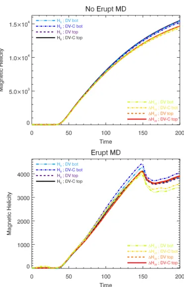
4.2. Total magnetic helicity evolution comparison
The comparative evolution of magnetic helicity for the seven dif-ferent flux emergence simulations is presented in Fig.5. In all cases, the helicity presents a smooth increase in time as helicity is injected into the system thanks to the continuous emergence. In the eruptive cases, the ejection of the flux rope from the sim-ulation domain is associated (very weakly in the strong arcade case) with a small decrease of HV after t ∼ 150. It is worth
noting that, compared to the injection of magnetic flux and en-ergy, the helicity accumulates much more smoothly and slowly. While more than 70% ofΦinj and 50% of Efree is injected into
the system between t = 30 and t = 50, only 10% of HV has
been injected into the system during that period. In all the flux emergence simulations studied here, the helicity injection is thus partly delayed compared to these other quantities. This delay be-tween the magnetic flux increase and the helicity accumulation agrees with the trend noted in observational studies of active re-gion emergence (Jeong & Chae 2007; Tian & Alexander 2008;
Liu & Schuck 2012).
The first significant result is that, unlike for magnetic flux and magnetic energy, magnetic helicity presents very significant differences between the different simulations immediately after the very start of the emergence. Each simulation is easily dis-tinguishable from the others as early as t ∼ 30. The magnetic helicity is much more of a discriminant than the energies and accumulated magnetic flux are. Magnetic helicity is thus able to characterize very well the magnetic configuration, as it depends
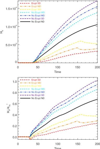
Fig. 5. Hv (top panel) and ˜H(bottom panel) evolution for the seven parametric simulations. The labels are similar to Fig.2.
not only on the strength of the surrounding field, but also on its orientation relative to the emerging flux rope.
As discussed in the Introduction, a large absolute value of the total magnetic helicity has been frequently suggested as a poten-tial proxy for flare eruptivity. In the framework of the present simulation, however, we notice that this is not the case. The top panel of Fig.5shows that the non-eruptive simulations all have a total absolute helicity |HV| several times higher than the
erup-tive one. Similarly, the normalized helicity (Fig.5, bottom panel) presents higher values for the non-eruptive cases. Our results in-dicate that a large value of |HV| cannot be used as a criterion for
eruptivity.
Looking at the influence of the arcade field strength, we note that there is an opposite behavior of the eruptive and non-eruptive simulations when it comes to the total helicity. For the non-eruptive simulations, the stronger the arcade field, the greater the total helicity |HV| (and ˜H), while for the eruptive
cases, the strength of the arcade and the intensity of |HV| are
anti-correlated.
The origin of these behaviors can be first explained by the fact that the weaker the arcade strength, the closer the system is to the no-arcade case (an infinitely weak arcade would e ffec-tively correspond to an absence of arcade field). This explains why, given the orientation of the arcade, the curves of HV and
˜
decreases. The curves of ˜Hand HV thus tend to become lower
or higher, respectively, for the non-eruptive and eruptive cases, as the arcade strength becomes lower.
This however does not explain why the orientation of the ar-cade leads to a higher HVin the non-eruptive case and lower one
for the eruptive simulations. This dependence originates from the fact that, unlike most quantities, magnetic helicity is intrinsi-cally non-local (Berger & Murdin 2000). When the flux rope is emerging, it not only advects its own helicity, but also instanta-neously exchanges helicity with the surrounding magnetic field. As we show in the following simplified toy model, the difference of HVbetween the different simulations is directly marked by the
mutual helicity shared by the emerging flux rope and the arcade field.
In the case of a system formed by two closed flux tubes, the total helicity is the sum of the proper helicity contained in each of the flux tubes, their self helicity, plus the helicity shared be-tween the flux tubes, their mutual helicity (cf. e.g.Berger 1984,
2003). In an analogous toy model, one can theoretically decom-pose the helicity of the present system between the self helicity of the emerging flux rope, HS,FR, the self helicity of the arcade
field, HS,Arc, and the mutual helicity shared between the
emerg-ing flux rope and the arcade field, Hmut:
HV = HS,Arc+ HS,FR+ Hmut. (12)
Initially, the flux rope not having yet emerged, the helicity of the system is solely given by the helicity of the arcade field and is expected to be null since the system is initially quasi-potential in the coronal domain (cf. Fig.3), independently of the strength of the arcade field: HV(t = 0) = HS,Arc ' 0. This is confirmed
by the measured values of helicity at the beginning of the simu-lations in all cases. Furthermore, the simulation with no-arcade field contains no mutual helicity. The values of HV in that case
should roughly represent the evolution of the self helicity of the flux rope field: that is, HS,FR(t) ∼ HV, No Erupt ND(t).
The differences in the curves of HV should therefore
orig-inate from the difference in Hmut. In the case of two closed
curved flux ropes, their mutual helicity is equal to the product of their magnetic flux weighted by their Gauss linking num-ber (Berger & Field 1984;Berger & Murdin 2000). Depending on the relative orientation of the curves, the linking number can either be positive or negative. In the present simulation, it is rea-sonable to argue that |Hmut| will be proportional to the product
of the flux of the magnetic arcade, ΦArc, and the flux of the
magnetic flux ropeΦFR. The flux of the emerging flux rope is
roughly constant between the simulations, and almost exactly in the initial phase of the emergence, before t ∼ 65 as shown by the evolution ofΦinj in Fig.2. For each simulation, the flux of
the arcade is directly given by the values of the flux initially, that is,ΦArc = Φini. The sign of the mutual helicity depends on
the relative orientation of the arcade and the emerging flux rope. When the arcade and the axial field of the flux rope have a pos-itive crossing, for the non-eruptive simulation, they should have a positive mutual helicity, while they should present a negative mutual helicity when the magnetic field orientation between the two has a negative crossing, for the eruptive cases. The helicity in the system should thus follow the relation:
HV − HV, No Erupt ND≡ HD∼ Hmut∼ ±ξΦArc, (13)
with ξ a constant of proportionality, and where the plus or minus sign applies to the non-eruptive or eruptive cases, respectively.
Qualitatively, this toy model predicts that the eruptive sim-ulation should have a lower HV than the no arcade case while
the non-eruptive one should have greater values. In addition, the stronger the arcade field, the further away HV is from the
no-arcade case. Quantitatively one also finds very good agreement between the Eq. (13) predicted by this simple toy model and the measured values of HV. During the main part of the emergence,
when the system is not too affected by the ejection of magnetic field, one measures at t= 75 that HD,No Erupt MD/HD,No Erupt WD=
1.46, and HD,Erupt MD/HD,Erupt WD = 1.51, while our toy
model theoretically predicts that these ratios should be equal to the ratio of the arcade strength between the medium ar-cade and the weak arar-cade case, that is, Φini,MD/Φini,WD =
3/2. Similarly, one has HD,No Erupt SD/HD,No Erupt MD = 1.30,
and HD,Erupt SD/HD,Erupt MD = 1.3, which should be equal to
Φini,SD/Φini,MD = 4/3 according to our toy model. In the case
of the non-eruptive simulations, the agreement improves as the emergence further develops.
The excellent agreement between these values demonstrates the importance of the mutual helicity between the emerging structure and the surrounding field, which, being added to or sub-tracted from the helicity advected by the emerging flux rope, sig-nificantly modifies the total amount of helicity. Even though the emerging structure is exactly the same in the seven simulations, the helicity budget is profoundly modified by the surrounding field. This highlights the importance of the surrounding environ-ment when considering the budget of magnetic helicity in flux emergence regions, unlike with more classical quantities such as energies.
While self and mutual helicity are useful theoretical con-cepts, they are in practice very difficult to use. The distinction between the emerging field and the arcade field is strongly sub-jective. When only considering a unique snapshot of one of the simulations, it is very difficult to objectively disentangle these two structures. It is even more difficult to directly compute each contribution. It is only thanks to the combined seven parametric simulations that we are able to compute the respective self and mutual contributions in the present study. Unlike Hjand Hpj, we
do not believe that it is generally possible to estimate these quan-tities from general datasets.
4.3. Current-carrying magnetic helicity evolution comparison We have seen that while the total magnetic helicity HV is very
discriminative of the different parametric simulations, its use to predict the eruptive behavior is limited, since for a given mag-netic flux injection, the eruptive simulations posses a lower to-tal amount of helicity. We will now discuss the evolution of the terms Hjand Hpjdecomposing the magnetic helicity (cf. Eq. (9))
and show that they constitute a very promising criterion of erup-tivity.
The time evolution of Hj and Hpj for the seven parametric
simulations is presented in Fig.6. We note that while the curves of Hpjpresent a relative distribution very similar to Hvbetween
the different simulations, the curves of Hjdiffer significantly.
Re-garding Hpj, the non-eruptive simulations have an evolution
sim-ilar to one another and simsim-ilar to HV both in shape and in
am-plitude. The differences in the evolution of Hpjfor the eruptive
simulations is more marked. While the weaker-arcade-strength case presents a relatively smooth increase, the stronger-arcade case displays slightly negative values during the first part of the emergence until t ∼ 100, and then some increase. As for HV, no
specific behavior before the onset of the eruption is noticeable in the evolution of Hpj.
The second main result of our study is that the curves of Hj
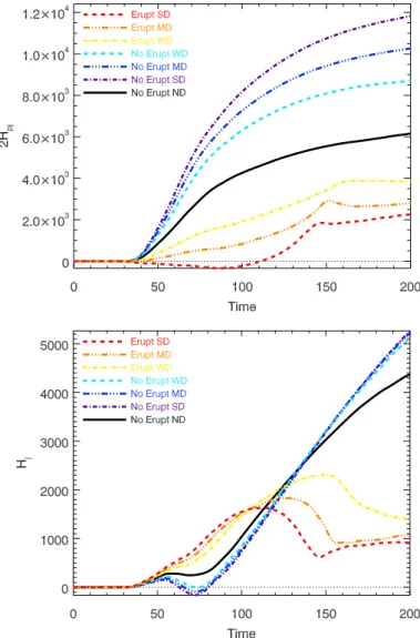
Fig. 6.Time evolution of 2Hpj(top panel), and Hj(bottom panel) for
the seven parametric simulations. The labels are similar to Fig.2.
(Fig.6, bottom panel). We note that the non-eruptive and erup-tive simulations present two very distinct groups. The simula-tion without surrounding magnetic field separates the two groups of simulations. For that simulation, after a slight increase for t ∈[30, 55], Hjpresents a plateau until t ∼ 75, before presenting
a slow and steady increase. The three non-eruptive simulations with a surrounding magnetic field present a relatively similar be-havior to one another. They are tightly grouped and are similar to the no arcade case. Instead of presenting a plateau between t = 30 and t = 50, Hjdecreases, even reaching negative values
before steadily increasing after t ∼ 75. These negative values may be related to the opposite direction of the current carrying field, mostly dominated by the emerging flux rope, and the vector potential of the potential field, mostly dominated by the arcade field. Unlike for HVand Hpj, the field strength of the arcade does
not seem to significantly influence the evolution of the values of Hj, although we note that the weak arcade curve is the one
closest to the no arcade case. This is probably because Hj, being
related to the current carrying field, is mostly influenced by the emerging flux rope rather than the initially potential arcade.
The eruptive simulations are tightly grouped with one an-other. Unlike the non-eruptive simulations, they present a quasi-steady increase in the first half of the simulation, before t ∼ 100. The curves then eventually reach a maximum, decrease, and then
remain relatively constant. While in the first part of the simula-tion, the curves only differ slightly in intensity, the timing of the maximum and the subsequent evolution is strongly influenced by the arcade field strength. The occurrence time of the maximum is anti-correlated with the strength of the arcade. The stronger the arcade, the earlier the peak of Hj. This is likely correlated to
the difference in the eruption time for the different eruptive sim-ulations. As noted in Figs. 12 of L14, the stronger the arcade, the earlier the flux rope moves and is eventually ejected, leav-ing the domain. The differences between the curves of Hjfor the
eruptive simulations have the following explanation: the stronger the external arcade, the larger is the flux available for reconnec-tion. For the emerging flux rope to erupt, the shell of stabiliz-ing field surroundstabiliz-ing it must be removed. Since the emergence timescale is dictated by the same photospheric evolution, more flux is available for reconnection for a given flux-rope emergence rate, the peeling of the outer shell is faster, and the time of erup-tion is earlier. Hence, the stronger the external dipole field, the earlier the start of the eruption. As a corollary, the longer it takes to erupt, the more flux rope emerges, therefore, the higher is the maximum of Hjthat can be reached.
While the eruptive simulations all display a higher value of Hj in the initial phase of the flux emergence, before t ∼ 100,
overall, the non-eruptive simulations are the ones that present the highest values of Hjin the later time of the evolution. Hence,
the value of Hjalone, while clearly being affected by the eruptive
behavior, cannot directly be used as an eruptivity criterion. The high value of Hj in the second phase of the simulations would
otherwise suggest that the non-eruptive simulations could be-come unstable, which does not agree with the dynamics observed at the end of these simulations. The situation is somehow similar to what was found for the free magnetic energy (cf. Fig.3, bot-tom right panel), with the difference being that helicity spreads the curves farther apart, that is, discriminates better between the different cases.
If Hjitself does not constitute an obvious eruptivity criterion,
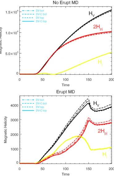
it nonetheless represents a significant portion of the total helic-ity of the system for the eruptive simulations, as can be seen in Fig.A.1for the medium arcade case, for example. Actually, the fraction of Hjto the total helicity is a key distinction between,
first, the eruptive and, second, the non-eruptive simulation, but also between the pre-eruptive phase and the post-eruptive phase of the eruptive simulations.
Figure 7 presents the ratio of |Hj| to the total helicity |HV|
for the seven parametric simulations. Because these curves cor-respond to a ratio, and because HV is roughly null before t ∼ 30
(magnetic flux only increases from that time on, we only plot values after that time in order to remove the spurious values resulting from the division by an infinitely small value. The non-eruptive curves are approximately constant throughout the simulation, with values that do not exceed 0.4. For the four non-eruptive simulations, Hj always remains a minor
contribu-tor to HV.
On the contrary, the eruptive simulations all present high val-ues of |Hj|/|HV| during the first phase of the simulation.
Imme-diately after the start of the emergence at t ∼ 30, the curves present a very fast rise, with a peak between t = 35 and t = 40. The values of |Hj|/|HV| even exceed 1, indicating an
opposite sign between Hj and Hpj. Helicity injection with
op-posite sign through the photospheric surface has been reported in several observed cases of eruptive active regions (Park et al. 2012; Vemareddy et al. 2012; Vemareddy & Démoulin 2017). Here, the level of the peak appears to be correlated with the strength of the arcade. It should be noted however that the values
Fig. 7.Time evolution of the helicity ratio |Hj|/|HV| for the seven
para-metric simulations. The labels are similar to Fig.2.
of HV are still very small at these times, amounting to less than
2% of the helicity eventually injected. After this initial peak, the values of |Hj|/|HV| remain high, relative to the non
erup-tive simulations, with values globally above 0.45. The level of |Hj|/|HV| is also directly correlated with the strength of the
ar-cade field, the stronger arar-cade field presenting a larger ratio than the medium arcade. The lower arcade presents the smaller ratio among the eruptive simulations, although still markedly higher than the non-eruptive simulation, with values two to four times higher than the no-arcade case, and more than five times higher than with the other stable runs. The curves remain relatively con-stant for some time, eventually decreasing after t ∼ 85 and fi-nally, after t ∼ 135 joining the group of the curves of the non-eruptive simulations.
The values |Hj|/|HV| are not only higher for the eruptive
sim-ulations compared to the non-eruptive ones, but they are only so during the pre-eruptive and eruptive phase of the simulations. In the post-eruption phase of the eruptive simulations, when the system is not eruptive, these values are back to a low value, be-low 0.4, typical of the non-eruptive simulations. Furthermore, during the eruptive phase, the ratio |Hj|/|HV| is also markedly
higher when the strength of the surrounding arcade is higher which, as noted by L14, is also related to a higher propensity for the system to erupt. Indeed, the higher arcade strength was associated with an earlier eruption of the system and a larger amount of reconnection. The ratio |Hj|/|HV| thus appears as a
very interesting criterion for qualifying and possibly quantifying the eruptivity of a system in solar-like conditions.
5. Eruptivity criteria comparison
In the previous sections, several scalar quantities that can char-acterize the magnetic field have been computed and their evo-lution analyzed and compared for the seven parametric simu-lations. Their ability to constitute a pertinent criterion of the eruptivity of the system has been qualitatively discussed. Only positive-defined quantities are being considered in the present study and constructed so that eruptivity could possibly be as-sociated with a high value of these proxies. Let us note that such positive criteria can always be built by the use of opposite or the inverse and modulus functions. In order to quantify the
quality of a good eruptivity proxy, we compute different param-eters that evaluate their distribution between the different simu-lations: the mean value, µ, and the relative standard deviation, Cv, of a given quantity at a given time for all seven simula-tions; the mean values, µErupt and µNo Eruptonly considering
re-spectively the eruptive/non-eruptive simulations, and their ratio η = µErupt/µNo Erupt.
A quantity which is not able to distinguish between the dif-ferent simulations will have Cv close to 0, as well as a value of η close to 1. This quantity thus does not possess the quality of a good proxy.
A high value of Cvindicates that this quantity is
discriminat-ing between the different simulations, although not necessarily their eruptive/non-eruptive character. Associated with a value of η close to 1, this means that this proxy is mostly sensitive to the strength of the surrounding arcade rather than the eruptivity.
A small value of η, close to 0, indicates that this quantity is significantly higher for the non-eruptive simulations. This gen-erally means that this quantity is not a good proxy for eruptivity. On the contrary, a high value of η, associated with a large value of Cv, is what is required from a good eruptivity proxy since it indicates that this quantity tends to be significantly higher for the eruptive simulations compared to the non-eruptive ones. For the eruptive simulations, a good eruptivity proxy should only have high values of Cvand η during the pre-eruptive and the eruptive phase and not during the post-eruptive phase.
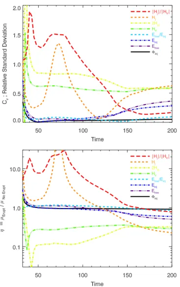
Figure8presents the evolution of η and of the relative stan-dard deviation between the different simulations. The curves of Cv show that the criteria based on magnetic flux and mag-netic energy, namely, Φinj, Einj, Efree, Efree/Emag, Efree/Einj are
not able to distinguish between the different simulations. Their relative standard deviation remains very small, <20%, during the pre-eruptive phase, for t ∈ [40, 70]. On the contrary the magnetic-helicity based proxies, HV, Hj, Hpj, |Hj|/|HV| present
high standard deviations indicating that the different simulations are strongly discriminating between these quantities. |Hj|/|HV|
possesses the noticeable property of being very high in the pre-eruptive phase and in the pre-eruptive phase, while decreasing in the post-eruptive phase.
The curves of η confirm again that the flux injection,Φinj, is
extremely similar for the eruptive and the non-eruptive simula-tions. The mean value of the eruptive simulations is constantly almost equal to the mean value of the non-eruptive ones. This quantity thus does not present any quality looked for in an erup-tive proxy. The same is true for Einj. The total volume helicity
HV and Hpj, while displaying distinctive behavior between
erup-tive and non-eruperup-tive, have very low values of η. This indicates that the eruptive simulation tends to have weaker values than the non-eruptive one. We observed in Sect.4, that the highest values of these quantities were eventually reached by the non-eruptive simulations during the post-eruption phase. It is therefore not possible to define a threshold from these quantities, which are thus poor eruptivity criteria.
The free magnetic energy, as well as Efree/Emag and
Efree/Einj, shows a weak tendency to be higher for the eruptive
simulation during their eruptive phase. Efreenonetheless has an η
value that drops markedly below 1 in the post-eruptive phase. As shown in Fig.3, the non-eruptive simulations present the highest values of Efreeduring that period. No threshold on Efreecan thus
be built in the present simulation framework. While being no-tably higher than 1 during the pre-eruptive phase, η(Efree/Einj)
decreases in the post-eruptive phase and becomes close to 1. Nonetheless, the value of η, of approximately 1.15 during the pre-eruptive phase, is not very high and thus may be of little
Fig. 8.Time evolution of the relative standard deviation, (Cv, top panel)
and ratios of the mean-eruptive and non-eruptive values (η, bottom panel) of several potential criteria for eruptivity. The (black continuous, purple dashed, blue dot-dashed, cyan dashed, green three-dot-dashed, yellow dot-three-dot-dashed, orange three-dot-dashed, red long-dashed) curve cor-responds, respectively, to the quantity (Φinj, Efree, Einj, Efree/Einj, HV,
2Hpj, Hj, |Hj|/|Hpj).
practical use with real data. In addition, as already noted in Sect. 3.2, the non-eruptive simulations reach greater values of Efree/Einjin the post-eruptive phase, even though no eruption is
present (cf. L13). The ratio Efree/Einj therefore does not likely
constitute a reliable proxy for eruption prediction.
The current magnetic helicity Hjpresents a high value of η
during the pre-eruptive phase, but then presents a low value dur-ing the post-eruptive phase, since the non-eruptive simulations present the highest values of Hj. Similarly to Efree, no threshold
on Hjcan be constructed that would enable the prediction of the
eruptivity of our parametric simulation.
Finally, Fig. 8 confirms that the ratio |Hj|/|HV| is an
ex-tremely efficient proxy of eruptivity for the simulations. This quantity presents clear variations of Cv from the pre-eruption phase to the post-eruption phase, and also presents a very high η, with values >5, in the pre-eruptive phase (for t ∈ [30, 120]). The values of η(|Hj|/|HV|) decrease during the eruptive phase
and eventually become close to 1 during the non-eruptive phase, for t > 150, indicating that the eruptive and non-eruptive
simulations are no longer distinguishable. This is expected since none of the simulations present any eruptive behavior during that last phase. An eruptivity threshold can easily be built from the ratio of |Hj|/|HV|. This quantity thus possesses a very strong
po-tential to allow the prediction of solar eruptions.
6. Conclusion and discussion
In the present study, we have computed and compared the mag-netic energy and helicity evolution of the coronal domain of seven parametric 3D MHD simulations of flux emergence, ini-tially presented in Leake et al. (2013, 2014). These numerical experiments, while only modifying a unique parameter – the strength and direction of the background coronal field – led ei-ther to a stable configuration or to an eruptive behavior with the ejection of a CME-like magnetic structure. These simula-tions represent a particularly interesting dataset that enables us to search for eruptivity criteria.
Following the method of decomposition of the magnetic en-ergy ofValori et al.(2013) and the method for computing rela-tive magnetic helicity presented inValori et al.(2012), we have computed different magnetic flux-, energy-, and helicity-based quantities throughout the evolution of the systems. As expected from the numerical setup, we noted that all the simulations presented a quasi-similar injection of magnetic flux. We have found that unlike magnetic flux and energy, relative magnetic helicity very clearly discriminates between eruptive and stable simulations.
We have however found that the total magnetic helicity was not correlated with a stronger eruptive behavior. Non-eruptive simulations, in fact, presented a higher absolute value of the total magnetic helicity compared to the eruptive ones. Using a toy model we have shown that the non-eruptive simulation possessed self helicity of the emerging flux rope of the same sign as the mutual helicity between the emerging flux rope and the coronal background field. Eruptive simulations presented a lower total helicity because the self and mutual helicities were of opposite sign.
Our results thus confirm those from Phillips et al. (2005), stating that the total magnetic helicity is not a determining factor for CME initiation and that there might not be a universal thresh-old on eruptivity based on total magnetic helicity. We however argue against their conclusion that helicity in general is unim-portant. Their setup, similarly to our eruptive cases, presents large helicities of opposite signs. The decomposition of helicity, if not its distribution, seems to be related to enhanced eruptive behavior. Using the helicity decomposition of the relative mag-netic helicity in the current-carrying magmag-netic helicity, Hj and
its counterpart 2Hpj, introduced byBerger(2003), eruptive and
non-eruptive cases present noticeably distinct behavior, with the eruptive simulations presenting significantly greater values of Hj
during the pre-eruptive phase.
Comparing the different quantities in their capacity to effi-ciently describe the eruptivity status of the different simulations during their evolution, we noted that while the ratio of the free magnetic energy to the injected magnetic energy, Efree/Einj is
higher for the eruptive simulations, in their pre-eruptive phase only, it presents two drawbacks: the values of this quantity are only marginally higher (by a few %) for the eruptive simulation, compared to the non-eruptive ones, and the non-eruptive simula-tions can reach values of a similar amplitude to the eruptive case. The definition of an eruptivity threshold seems to be difficult to determine with such a quantity.