HAL Id: tel-00311845
https://tel.archives-ouvertes.fr/tel-00311845
Submitted on 21 Aug 2008HAL is a multi-disciplinary open access archive for the deposit and dissemination of sci-entific research documents, whether they are pub-lished or not. The documents may come from teaching and research institutions in France or abroad, or from public or private research centers.
L’archive ouverte pluridisciplinaire HAL, est destinée au dépôt et à la diffusion de documents scientifiques de niveau recherche, publiés ou non, émanant des établissements d’enseignement et de recherche français ou étrangers, des laboratoires publics ou privés.
between a magnetized young star and its accretion disc.
Nicolas Bessolaz
To cite this version:
Nicolas Bessolaz. Magnetohydrodynamic simulations of the interaction between a magnetized young star and its accretion disc.. Astrophysics [astro-ph]. Université Joseph-Fourier - Grenoble I, 2008. English. �tel-00311845�
JOSEPH-FOURIER TECHNOLOGY
DISSERTATION
by
Nicolas B
ESSOLAZ to obtain the degrees ofDOCTOR OF THE JOSEPH-FOURIER UNIVERSITY and
DOCTOR OF THE EINDHOVEN UNIVERSITY OF TECHNOLOGY Specialty : ASTROPHYSICS – PHYSICS & DILUTE MEDIA
Magnetohydrodynamic simulations of the interaction
between a magnetized young star and its accretion disc
Thesis defense on May 29th 2008 with the following dissertation committee
Mrs. Marina ROMANOVA Referee
Mrs. Silvia ALENCAR Referee
Mr. Jean-Louis MONIN Chairperson
Mr. Jonathan FERREIRA Supervisor at LAOG
Mr. Niek LOPES CARDOZO Supervisor at the FOM institute
Mr. Rony KEPPENS co-Supervisor at CPA
Mr. Jean-François DONATI Examinator Mr. Richard van de SANDEN Examinator
PhD thesis prepared within the SHERPAS and FOST teams at the Laboratory of AstrOphysics of Grenoble (France), the Center for Plasma Astrophysics team in Leuven
(Belgium) and the Plasma Physics group at the FOM institute Rijnhuizen (The Netherlands).
star-disc interaction, stellar formation, accretion
discs, numerical methods, MHD.
PhD thesis — Grenoble I University (Joseph-Fourier) and Technische Universiteit Eindhoven (TUE)
ABSTRACT :
Nowadays, observation of slow rotators (3-8 days period) in star forming regions is still puzzling for accepted theoretical models, since efficient physical processes have to be considered to extract angular momentum brought by circumstellar matter accreting onto these stars, which moreover are still in a contraction phase. The interaction of the stellar magnetic field with its surrounding accretion disc is often presented as a possible explanation for this issue. In this thesis, we first present the state of the art of the star-disc interaction problem highlighting both the observations, theory and previous simulations which support it. Then, we model this interaction between a dipolar stellar magnetic field and a consistent accretion disc model including dissipative effects and we carry out simulations using the Versatile Advection Code (VAC) which solves the equations of magnetohydrodynamics.
The first goal of this thesis is to re-examine the conditions required to steadily deviate an accretion flow from a circumstellar disc into a magnetospheric accretion column onto a slow rotating young forming star. A new analytical and predictive criterion on the truncation of discs by the dipolar stellar field is derived stressing the importance of the disc thermal pressure. The physics of accretion columns is explained in detail. We confirm the numerical results of Romanova et al. (2002, ApJ, 578, 420) and find accretion funnels for stellar dipole fields as low as 140 G in the low accretion rate limit of 10−9M
yr−1. With our present numerical setup with
no proper disc magnetic field, we found no evidence of winds, neither disc driven nor X-winds, and the star is only spun up by its interaction with the disc in this slow rotation range.
The second goal of this thesis is to test the robustness of magnetospheric accretion by doing a parameter space study varying the stellar magnetic field and rotation rate, and the amount of dissipation within the disc. Accretion columns are always present when the inner parts of the disc rotates quicker than the star, with oscillations of the truncation radius in presence of disc viscosity. The stellar accretion rate diminishes when the stellar magnetic field strength or rotation rate increases, which reduces the angular momentum brought onto the star. However, a disc-locking state is not clearly found, but stellar winds can be another possibility to efficiently extract angular momentum. This is already seen in our simulations even though we do not control here the mass loading into the stellar corona.
RESUME :
L’observation de rotateurs lents dans les régions de formation d’étoiles reste encore aujourd’hui une énigme puisque les mécanismes physiques sous-jacents permettant d’expliquer une extraction efficace du moment cinétique apporté par l’accrétion de matière autour de ces étoiles, qui sont de plus toujours en phase de contraction, ne sont pas clairement identifiés. L’interaction du champ magnétique de ces étoiles avec le disque d’accrétion en rotation autour d’elles est souvent présentée comme la solution pour ce problème. Dans cette thèse, je dresse d’abord le panorama d’ensemble qui justifie ce paradigme d’interaction étoile/disque tant du point de vue observationnel que théorique. Ensuite, je modélise cette interaction en prenant en compte le champ magnétique stellaire considéré ici comme dipolaire et un disque d’accrétion en incluant les effets dissipatifs dans ce dernier. J’effectue alors des simulations
numériques en utilisant le code VAC (Versatile Advection Code) qui résout les équations de la magnétohydrodynamique.
Le premier objectif de cette thèse est de ré-examiner les conditions nécessaires pour détourner de manière permanente l’écoulement d’accrétion du disque dans une colonne d’accrétion, dans le cas d’une étoile jeune tournant lentement. Un nouveau critère analytique et prédictif est obtenu pour trouver la position de troncation du disque par la magnétosphère de l’étoile considérée dipolaire et je montre l’importance du gradient de pression thermique dans le disque. La physique des colonnes d’accrétion est expliquée en détail. On confirme les résultats numériques de Romanova et al. (2002, ApJ, 578, 420) en trouvant des colonnes d’accrétion pour des champs magnétiques stellaires ayant une composante dipolaire aussi faible que 140 G dans le cas limite de faible taux d’accrétion sur l’étoile autour de 10−9M
par an. Avec le choix de
notre configuration initiale sans champ magnétique propre dans le disque, je ne trouve pas véritablement de vent de matière, qu’il soit étendu dans le disque ou concentré autour de la troncation du disque comme décrit par le modèle de vent X, et l’étoile est toujours accélérée par l’interaction avec son disque dans le cas où on a un rotateur lent.
Le deuxième but de cette thèse est de tester la robustesse de l’accrétion magnétosphérique en faisant une étude de l’espace des paramètres où on fait varier le champ magnétique et la vitesse de rotation de l’étoile ainsi que l’importance des effets dissipatifs dans le disque. Les colonnes d’accrétion sont toujours présentes quand les parties internes du disque tournent plus vite que l’étoile avec des oscillations du rayon de troncation du disque en présence de viscosité. Le taux d’accrétion sur l’étoile diminue quand le champ magnétique stellaire ou sa vitesse de rotation augmente, ce qui réduit l’apport de moment cinétique à la surface de l’étoile. Pourtant, je ne trouve pas clairement une configuration où la rotation de l’étoile est fixée à une faible valeur par la présence du disque et la présence de vents stellaires semble être une autre possibilité d’extraire efficacement du moment cinétique comme c’est déjà entrevu dans mes simulations même si je ne contrôle pas ici le taux de perte de masse dans le vent.
It is now time to thank all the people who support me in the last years to achieve this thesis. First of all, I would like to thank my supervisors. Rony Keppens brought me all his expertise in numerical simulations, above all at the beginning of the thesis guiding me in this complex field where I was nearly a beginner, but also then letting me do my own experience trusting me. I would like to thank him for the fruitful discussions we had about my simulation results but also for his pragmatic view which helps me to advance when I was too cautious and I had doubts about my work. Jonathan Ferreira, although not being used to numerical experimentations, took time to discuss about the simulations and I would like to thank him for his wide background in Physics which has been a source of inspiration for my own research. Jérôme Bouvier and Catherine Dougados allow me to obtain the best observational background of these versatile YSO.
But also this thesis enables me to work in different European institutes which was very wealthy. I will always remember my office in the Rijhnuizen castle surrounded by a very beautiful park with a lot of hens and ducks, the Leuven city very animated during nights with very tasty beers. I was also very glad to share the second floor of LAOG with many other students who put a very pleasant atmosphere. I would like to thank the Nicolas’ team, Tim, Benoît, Rémy and Philippe but also the persons in the same position like me i.e. Myriam, Geoffroy, Oscar and Guillaume. I would like to specially thank Claudio for his friendship and collaboration to make comparison of our work with the PLUTO code. It was really helpful to get confidence in simulations for this difficult numerical work but also to identify their limits due to the different numerical schemes used. Finally, I would like to thank my parents and my sisters for encouraging me and helping me to overpass difficulties in the last months to finally write this thesis and also all people I do not cite here but I met during these years.
Acknowledgements 7
List of Figures 11
Introduction 1
CHAPTER 1. Astrophysical context 4
1. Observational overview for T-Tauri stars 5
§ 1. Basic properties 5
§ 2. Disc accretion rates and clues for inner disc holes 8
§ 3. Spectral features 10
§ 4. The issue of the slow rotation 12
§ 5. Stellar Magnetic field constraints 15
2. Theoretical background of the star-disc interaction 17
§ 6. The global picture of an extended star-disc interaction 18
§ 7. Variability of the disc truncation radius 20
§ 8. The physics of stationary funnel flows 21
§ 9. The importance of the disc diffusivity for the stellar rotational evolution 28 § 10. Ejection processes to solve the angular momentum issue? 30
CHAPTER 2. Numerical MHD 35
1. Numerical methods 36
§ 11. Finite volume discretization 36
§ 12. The CFL condition 37
§ 13. The choice of the numerical flux 38
§ 14. Variables reconstruction, slope limiters and high resolution schemes 42
§ 15. The issue of positivity 43
§ 16. Methods for multidimensional systems 43
§ 17. Discretization in axisymmetry 44
§ 18. The ideal MHD equations 44
§ 19. Numerical techniques to ensure the divergence-free property of the magnetic field 45
§ 20. Boundary conditions 47
2. The VAC code 48
§ 21. Description of the code 48
§ 22. TVD Lax Friedrichs scheme 49
§ 23. Practical details of our simulations 49
3. Review of previous numerical simulations of star-disc interaction 51 § 24. Long term evolution without resolving the disc structure 51 § 25. 2.5 D simulations with the dynamical evolution of the disc 53
§ 26. 3D simulations 59
CHAPTER 3. MHD model of the star-disc system 63
1. The validity of MHD in this context 63
2. The accretion disc model 64
§ 27. Design of an equilibrium initial condition 64
§ 28. Temperature in simulations 66
§ 29. The issue of the viscous torque 66
§ 30. On the α disc prescription in cylindrical coordinates 67 § 31. The viscous accretion disc in Romanova et al. (2002) 68
§ 32. Viscous hydrodynamic simulations 70
§ 33. The diffusivity within magnetized accretion discs 73
3. The stellar magnetosphere 76
§ 34. Design of boundary conditions 76
§ 35. Implementation of the splitting method for the magnetic field 79
CHAPTER 4. The truncation of the disc and funnel flow formation 81
1. The disc truncation radius 82
2. Numerical experiments 85
§ 36. Equations and numerical setup 85
§ 37. Boundary conditions 85 § 38. Initial condition 86 § 39. Reference values 87 § 40. Methodology 89 § 41. Results 90 3. Conclusion 104
CHAPTER 5. Parameter space study of the star-disc interaction 107
1. Accretor regime (rt <rco) 108
§ 42. Role of viscosity 108
§ 43. Influence of resistivity on star-disc connectivity 112 § 44. Relation between the stellar accretion rate and the star-disc system parameters 115
2. Propeller regime ( rt >rco) 120
§ 45. Dynamical evolution 121
§ 46. Ejection properties 122
§ 47. Angular momentum balance 122
3. Conclusion 123
Conclusion 125
Contributions 133
1 Optical spectra for late spectral type K T-Tauri stars with an increasing level of emission lines and veiling from the bottom to the top. The star TAP57 is classified as a WTTS (from Bertout 1989). One clearly distinguishes the Hα line at 6563 Å and also the UV
excess below 4000 Å. 6
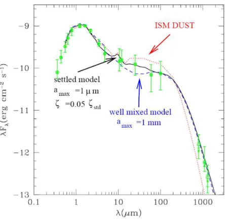
2 SED of disc models for different properties of the dust component (the size distribution follows n(r)∝r−3.5) : well-mixed ISM dust (dotted line), well mixed grains with rmax=1 mm (dashed line) and dust settling from rmax = 1 µm at the disc surface to rmax = 1
mm at the disc midplane (solid line). Data points represent the median observed SED of CTTS in Taurus obtained with the IR spatial telescope Spitzer and corresponds to the following stellar parameters : M∗ = 0.5M , R∗ = 2R and a mean accretion rate of
10−8M
.yr−1. One can distinguish the stellar component below 2 µm and the silicate
band at 10 µm. One clearly sees that spectra favour a settlement of dust in the disc
midplane (from d’Alessio et al.2003). 7
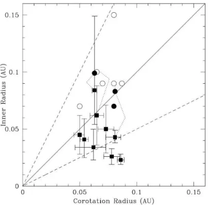
3 Gaseous inner disc radii for TTS from CO fundamental emission (filled squares) compared with corotation radii for the same sources. Also shown are dust inner radii from near-infrared interferometry (filled circles; Akeson et al., 2005a,b) or spectral energy distributions (open circles; Muzerolle et al., 2003). The solid and dashed lines indicate an inner radius equal to, twice, and 1/2 the corotation radius. The points for the three stars with measured inner radii for both the gas and dust are connected by dotted lines (from
Najita et al. 2005). 9
4 Different Hα and HeI lines for DR tau ordered by the magnitude of the veiling in the R
band rR (from Beristain et al. 1998). For high veiling, we can see P Cygni profiles for Hα
lines indicative of an ejection process and Inverse P Cygni profile for HeI lines for low veiling which probe accretion phenomena. Negative velocities measured in the stellar
rest frame correspond to blueshifted motions. 10
5 Evolution of an Hα line profile on a stellar period timescale with a modification of the
blueshifted part. Julian time is given for each line (from Alencar et al. 2000). 12 6 Correlation between the blueshifted and redshifted absorption components of the Hα
line in AA Tau (from Bouvier et al. 2003). This can be explained by the expansion of the magnetosphere which increases the blueshifted velocities along the line of sight while
the accretion is reduced. 13
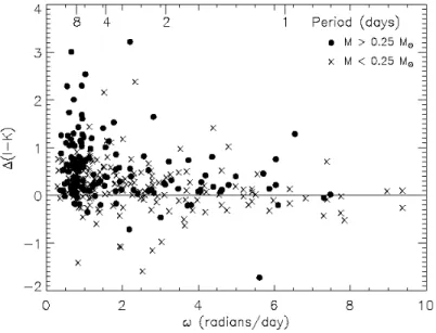
7 Infrared excess emission measured by I-K as function of the stellar angular velocity ω (or periods). One clearly observes a concentration of slow rotators with significant infrared excess for not too low mass stars (M>0.25 M ) (from Herbst & al. 2002). 13
8 Rotation periods distribution function in NGC 2261 (a) and the Orion Nebula Cluster (b) for the stellar mass range M∗ ∼0.25−1.2M (from Herbst et al. 2007). 14
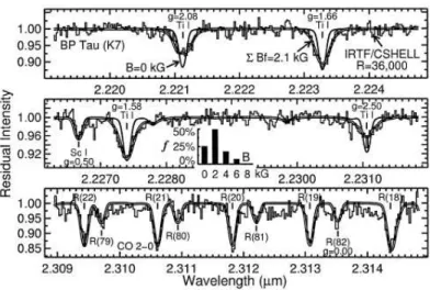
9 Spectrum of BP Tau (histogram) with a fitted magnetic model (double line) taking into account a distribution of magnetic field strength reaching 6 kG with different filling factors and with a mean field of 2kG covering half of the stellar surface (from Valenti & Johns-Krull 2004). One can notice that a non magnetic model (single line) does not
explain the broadening of Ti I lines but agrees for CO lines. 16
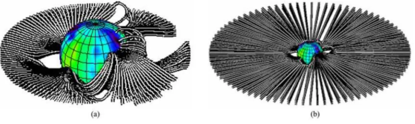
10 Magnetic field lines extrapolation for a CTTS that resembles LQ Hya (a) or AB Dor (b)
(from Gregory et al. 2006). 17
11 Schematic picture of the Ghosh & Lamb model (adapted from Ghosh & Lamb 1978). 19 12 Equipotential lines (black lines) in the (r,z) plane for the effective gravity in the case of a
rigid rotation of the magnetosphere. The values represent the opposite of the effective potential. We identify the corotation at 1.6. The red lines corresponds to magnetic field lines for a pure dipolar field and the brown lines represents circles. Along a given field line, accretion is possible if the opposite of the effective gravity keeps increasing from the equatorial plane towards the star. We find that polar accretion is possible only for
r ≤1.4 corresponding to rt <0.875rco. 23
13 Equipotential lines (black lines) for the effective gravity Ve f f in the case of differentially
rotating magnetic field lines with the same legend as in Fig. 12. The polar accretion is possible here only for r≤1.1 corresponding to rt< 0.69rco. 24 14 Contour of the normalized Bernoulli integral E’ for a disc with an aspect ratio 0.054
(A = 1.5×10⁻³) and a magnetic field line anchored below the corotation (C = 0.6) as function of the Mach sonic number and the distance along the funnel flow in units of sd = 1−R0. The disc midplane corresponds to sd = 0 and the stellar surface is on the
right side. The sonic point corresponds to the saddle point which is localized at the disc
midplane. We find solutions for initial sonic speeds. 25
15 Contour of the Bernoulli integral for a disc with an aspect ratio 0.054 (A = 1.5×10⁻³) and a magnetic field line anchored at corotation (C =1). We now find solutions only for initial supersonic speeds with a sonic Mach number higher than 5. 26 16 Isocontours of E’ with the same disc aspect ratio (A=1.5×10⁻³) as previously zooming
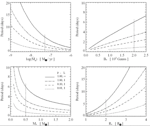
in near the sonic saddle point for (A) C=0.6 (same case as Fig. 14) and (B) C=0.7 using a different scale in units of h for the position along a magnetic field line. 27 17 Equilibrium rotation period as a function of ˙Ma,B∗,M∗ and R∗ (from Matt &
Pudritz 2005). The solid line corresponds to a global closed magnetosphere (with γc ∼ ∞ and p = 1) whereas the other cases consider a partial opening of the magnetic field taking γc = 1 and different values for the diffusion parameter
p =0.01(dotted lines), 0.1(dashed lines)and 1(dash−dotted lines). 29 18 Magnetic configuration of the star-disc system including a proper disc magnetic field
(from Ferreira, Dougados & Cabrit 2006). Left : Parallel configuration with an MHD X
point. Right : Anti-parallel configuration. 30
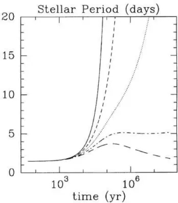
19 Stellar period evolution for an initial condition with f=0.1, λ = 3, R∗,0 = 4R ,
field index n=1 (solid),n=3.41 (dashed), n= 3.87 (dotted), n=4.4 (dash-dotted) and n=5
(long-dashed) with no stellar dynamo (from Ferreira et al. 2000) 33
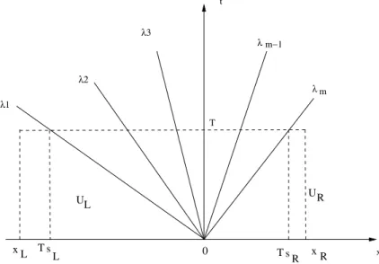
20 General solution of the Riemann problem in the (x,t) plane. At the cell interface located at x=0, we represent the propagation of the different wave characteristics of the system considered. The information transported by the fastest waves reaches distances equal to sRT and sLT at the end of the time step T which is lower than the cell width [xL, xR] due
to the CFL condition. 40
21 Spatial reconstruction of variables with slope limiters. 42
22 Typical grid used in simulations including the ghost cells layer. The resolution is 174×104 in the radial and orthoradial directions respectively. The intersections in this plot correspond to the cell centers. We can notice the symmetry of the rows at each side
of the axis and the equator. 50
23 Series of snapshots at t=0,10,20,80,160 Ω−1
K (r = 1)showing the density distribution and
the poloidal magnetic field lines (above) and the contours of the toroidal magnetic field (below) for a stellar outflow rate twice lower than the disc one (from Fendt & Elsner 2000). The accretion disc midplane is the vertical axis and the normalized spatial unit corresponds to 2 R∗. From an initially distorted dipolar field, the magnetic field for the stationary state corresponds to a nearly spherical topology. One can remark the formation of several plasmoids in the current sheet oriented at 45◦ with respect to the
disc midplane and also knots within the axial jet. 52
24 Two types of simulation with different magnetic initial configuration with the resulting accretion process used in Miller & Stone (1997). Above : A pure dipolar field (even strong) gives direct equatorial accretion due to efficient angular momentum extraction within the disc by the MRI well visible with the kink on the magnetic field lines in the disc. Below : A disc magnetic field is added with the same polarity as the stellar magnetic moment which gives rise to an X point allowing polar accretion. Time unit
corresponds to the Keplerian period at the stellar surface. 54
25 a- Time evolution of an ideal MHD simulation with the setup defined in Romanova et al. (2002) including a viscous disc (αν = 0.02) and Rco = 1.7 (from Long et al. 2005).
b-Angular momentum fluxes brought by matter fm and by the magnetic field fB. The
reversal of sign of the angular momentum flux transported by the magnetic field is well
below the corotation at r ∼1.2. 56
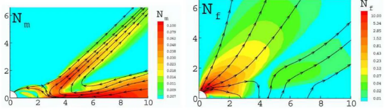
26 Angular momentum fluxes brought by matter Nm and by the magnetic field Nf in the
propeller regime (from Romanova et al. (2005)). 57
27 Topology of the funnel flow accretion as function of misalignment angle θ and the corresponding hot spot position at the stellar surface. Simulation from Romanova et al.
(2004b). 59
28 Light curves as function of the inclination angle for a configuration with a misalignment angle θ = 45◦. Bottom : the energy flux distribution in the hot spots are shown at the stellar surface for different phases of a rotation period. Simulation from Romanova et al.
29 Fraction of the star f covered by hot spots as function of accretion rate ˙M and density levels ρ in the hot spots. The reference values are ˙M0 = 1.9×10⁻⁷M yr−1 and
ρ0=4.9×10⁻¹²gcm−3. Simulation from Romanova et al. (2004b). 60 30 (a) Density distribution in the equatorial plane showing penetration of tongues of matter
through magnetosphere in the presence of disc viscosity with αm =0.1. (b) Contours of
the velocity profile within the funnel flows and tongues for a constant density surface
(from Kulkarni & Romanova 2007). 61
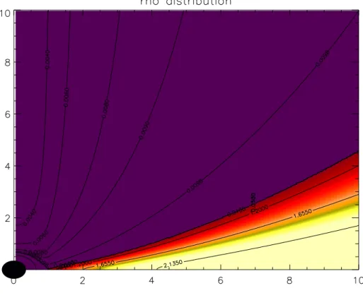
31 Density distribution in normalized units corresponding to the initial condition defined
in Romanova et al. 2002 with a truncation radius at r=1. 69
32 Vertical profile of the radial velocity for α = 0.01 at r=2 from Eq. (31.73). One has strong inflow throughout the disc. The sonic Mach number is really big reaching ms =0.02 in the disc midplane with respect to standard disc model where one expects
ms=αe∼0.001. 70
33 Accretion rate deduced from Fig. 32 using the initial condition of Romanova et al. (2002)
in normalized units for α =0.01. 70
34 Viscous simulation with αν = 0.4 and taking into account only τrφ. Left panels shows
the density distribution in log scale for different times given in periods at r=1 and right panels shows the distribution of sonic Mach numbers within the disc. We see outflow in
the disc midplane. 72
35 Top- Evolution in time of the accretion rate for αv =0.4 and taking into account only τrφ.
Bottom- Evolution in time of the vertically averaged sonic Mach number. 73 36 Viscous simulation with αν = 0.4 and taking into account the complete viscous stress.
Left panels shows the density distribution in log scale and right panels shows the distribution of sonic Mach numbers within the disc. We have no longer back flow in the
disc midplane. 74
37 Different vertical diffusivity profiles as defined in the text : f1(x)(dashed), f2(x)(solid)
and f3(x)(dashed-dotted). 75
38 Main characteristics of some CTTS such as their mass M∗, radius R∗, accretion rate ˙M,
period Prot, corotation radius rco, mean magnetic strength ¯Bobswhich includes small-scale
field often very different from the large scale field Bdip,obs and the resulting theoretical
truncation radius rt,thcalculated from Eq. (35.104) assuming ms ∼ 1 and B∗,dip =140G
(values into brackets are calculated using maximal observational constraints based on Valenti & Johns-Krull 2004, Daou et al. 2006, Donati & al. 2007, Yang et al. 2007) in comparison with truncation radius rd
t derived from Najita & al. (2003) (values into
brackets are calculated for the stellar mass given in this table). 84 39 Angular velocity of the magnetic surfaces at the stellar surface after 10 stellar periods.
The normalized angular velocity of the star is 0.35. We observe a slightly discrepancy (lower than 4%) localized within the accretion column between 55◦and 70◦. 86
40 Resistive MHD simulation for a 5 days period CTTS with B∗ =141G and αm =0.1 after t=0,5.1,10.2,15.3,20.4,25.5 Keplerian periods at the disk inner edge corresponding to a physical time of 1.5 months. We show the density distribution in the computational domain using a log scale. The black lines draw the magnetic field lines and the black
arrows represent the velocity field. The white line on the first snapshot represents an initial magnetic field line anchored at rco. We also superimpose a part of the
computational grid to show the good resolution we have near the truncation radius. An accretion column is formed between rtand rbf(see definitions in text) and one observes
the expansion of the poloidal magnetic field and transient disc ejecta. The accretion rate at the stellar surface is equal to 1.9.10−9M
.yr−1 for P=5 and stabilizes towards
0.91.10−9M
.yr−1at P=15. No X-winds are formed and the star is being spun up. 88
41 Projection of the forces in normalized units along a magnetic field line in the middle of the accretion column, for run (s1) at t = 10. We represent the gravity FG, the centrifugal
force FC, the thermal pressure gradient FP, the poloidal magnetic force FM and the total
force Ftotas function of the curvilinear coordinate s. The disc midplane is located at s=0 and the disc surface corresponds to s ∼ 0.2. Gravity begins to dominate the dynamics only at some distance between the disc and the star (s ∼1.2 at the stellar surface). 89 42 Angle between the poloidal velocity vector and the magnetic field one as function of the
curvilinear distance s along a magnetic field line in the middle of the accretion column. One clearly sees the transition between the resistive disc and the ideal MHD funnel flow
at s∼0.2. 90
43 Same caption as Fig. 41 for the series of snapshots presented in Fig. 44. We can remark the build up of the vertical thermal pressure force between t=0.8 and t=1.4 and also the less increase of the gravitation force due to the dipole deformation caused by accretion. 91 44 Same caption as in Fig. 40 with a series of snapshots focused on the development of a
funnel flow corresponding to the force balance presented in Fig. 43 92 45 Density distribution at the stellar surface versus the angular distance from the equatorial
plane (on the left hand side) as a function of time. 93
46 Toroidal magnetic field distribution at the stellar surface versus the angular distance
from the equatorial plane. 93
47 Angular velocity distribution at the stellar surface versus the angular distance from the
equatorial plane, for consecutive times during the evolution. 94
48 Radial distribution of Bz(solid line) with respect to the initial dipole distribution (dashed
line). 95
49 Top - Evolution in time of the position of the truncation radius rt(solid lines) for a set of
resistive MHD simulations with B∗ = 141G, P∗ =5.1days and αm= 0.1 and a different
initial truncation radius. The time unit is the Keplerian period at r=1. All runs converge towards a truncation radius rt ∼ 1.2 (solid lines). Dash-dot lines represent, for each
simulation, the radius r1where β= 1. We report also the radius rbf(dashed line) which
indicates the base of the funnel flow, rt,max(dashed line) and rt,minfor our reference run
(s1). Bottom - Evolution in time of the sonic Mach number at the base of the funnel,
ms(rbf), for run (s1). 96
50 Radial distributions of density ρ, angular velocities Ω (real) and ΩK (Keplerian) and
sonic Mach number ms = ur/Csat the disc midplane, for run (s1) after 17 keplerian
51 Simulation with the boundary conditions of Romanova et al. (2002) for the inner
boundary, i.e. free boundary conditions for Bθand Bφand fixed Brcomponent. 98
52 Top - Evolution in time of the accretion rate ˙Ma(dash dotted line), angular momentum
flux transported by matter ˙Lm(solid line) and by the magnetic field, computed for the
closed ˙Lf c (dash line) and open ˙Lf o (dotted lines) field lines. The units are normalized
and the two hemispheres are taken into account. 99
53 (A)-Sonic (dotted line), Slow-Magnetosonic (dashed line) and Alfvénic (dash-dotted line) Mach numbers within the funnel flow along the same magnetic field line at t=10 as in Fig. 41. (B)-We represent the free-fall velocity profile vf f, the transverse velocity to the
funnel-flow vn, the Slow-Magnetosonic speed vSM, the poloidal velocity parallel to the
magnetic field vpand the Alfvénic speed vA. 100
54 MHD invariants as defined in chapter 1 along a central magnetic field line in the funnel
flow at t=17. 101
55 Location of the slow magnetosonic surface within the funnel (blue dashed-dotted line) at t=9.4. We also plot some magnetic field lines (black solid lines) and specially those at the edges of the accretion column (black dashed lines) showing the distorted field. One can remark that the flow within the disc is super-slow and becomes sub-slow at r<1.2 near the truncation radius at r=0.8. Material launching along the opened field lines becomes
super-slow above the disc near z∼0.5. 102
56 Evolution of density, temperature and angular velocity within the funnel flow along a
central magnetic field line 103
57 Same caption as in Fig. 49 with B∗ = 141G, P∗ = 5.1days and two different disc
diffusivities characterized by αm = 0.1 (green curve) and αm= 0. (red curve). The two
runs converge towards the same truncation radius rt∼1.1. 104
58 Resistive MHD simulation for a 5 days period CTTS with B∗ = 141G and αm= 1 after
t=10. One shows the density distribution in the computational domain using a log scale
as well as flow vectors and magnetic field lines. 105
59 Forces in normalized units within the accretion column near the disc surface in the case αm =1. We can remark that the gravity in this case is always negative since the dipole is
less distorted by accretion. 105
60 Resistive MHD simulation with B∗ =703G and αm= αv=0.1. The density distribution
is drawn, the black lines show the magnetic field lines and the black arrows the velocity field. The white line in the initial condition indicates the magnetic field line corotating with the star which has a period of 17 days. After the first dynamical accretion, we observe the formation of a current sheet due to the expansion of the poloidal magnetic field with a strong ejection linked to a strong deformation of the closed magnetosphere and then a new accretion phase with a powerful accretion column. Finally, the magnetosphere is again deformed by both accretion and expansion of the magnetic field
due to the differential rotation. 109
61 Variation of the stellar accretion rate with time for a weak field case (a: B∗ =141G) and a strong one (b: B∗ = 703G). First, one can remark the long term decrease corresponding
a reversed trend for the stronger case because the magnetic braking timescale is longer as the initial truncation radius is further. Then, the period of the magnetospheric cycle is shorter for the weak field case, namely it is around 7 periods with respect to the stronger
case, where it is around 10 periods. 110
62 Oscillation of the truncation radius in presence of viscosity for B∗ =703G. We clearly see a complete cycle of the magnetosphere after the first dynamical accretion. One also sees a trend to a decreasing of the truncation radius due to the effect of the magnetic braking which increases with the opening of the magnetic field in the disc outer parts. 111 63 Radial profile of the accretion rate in the disc midplane for three different times showing
the time-dependent magnetospheric accretion for the strong field case. t=10 corresponds to the maximum of the first accretion phase, t=15 show the end of this first accretion with accumulation of matter at the disc inner edge and finally one sees the second accretion,
which is more powerful due to the greater accumulation of mass. 112
64 Ideal MHD simulation with the initial condition of Romanova et al. (2002) for a 10 days period CTTS with B∗ = 124G and αv = 0.02. The density distribution is drawn and the black lines show the magnetic field lines. The white line in the initial condition indicates the magnetic field line corotating with the star. One clearly obtains an accretion column after 5 periods. Notice however the excretion in the disc midplane caused by the bending of the magnetic field lines due to greater accretion at the disc surface. This finally produces reconnection in the disc midplane when the field lines are too stretched
radially which disrupts the disc into two parts. 113
65 We reproduce here a snapshot from Romanova et al. (2002) with the same parameters as in our simulation except a stronger field strength with B∗ = 1100G. One can see the excretion in the equatorial plane and accretion in the upper parts which distorts the magnetic field lines in the same way as in our simulation but less quickly as in our
weaker field case. 113
66 Projection of the forces in normalized units along a magnetic field line in the middle of the accretion column, at t = 10 for the simulation shown in Fig. 64. We represent the gravity FG, the centrifugal force FC, the thermal pressure gradient FP, the poloidal
magnetic force FMand the total force Ftotas function of the curvilinear coordinate s. The
disc midplane is located at s =0. 114
67 Resistive MHD simulation for a 4 days period CTTS with B∗ =141G and αm = αv= 1.
We achieve a restricted star-disc connection limited to the funnel flow as in our reference simulation in Chap. 4 even though we increase the disc dissipative effects by an order of magnitude. The visco-resistive parameters now reach their upper limit of physically
possible values for turbulence. 115
68 Resistive MHD simulation for a 4 days period CTTS with B∗ =224G and αm = αv= 1.
We achieve a transient star-disc connection beyond the corotation radius till r=2.5 and a disc wind configuration further. On longer times though, the disc is expelled by the negative magnetic torque which diffuses inwards till r=1.1 well below the initial
69 Radial distribution of the toroidal field near the disc surface at t=2. We see the first reversal of sign for the toroidal field at r=1.2 instead of its expected position at the corotation (r=1.6). Then, we have a negative field till the magnetosphere is opening at
r=2.2. 117
70 A series of simulations with Ω = 0.1 corresponding to rco = 4.6, αv = αm = 0.1 and
varying the magnetic field strength B∗. One reports the maximum stellar accretion rate
˙
M∗,max, the disc truncation radius measured at this time rt,min with comparison to the
theoretical one rt,th, the magnetosphere cycle period observed , the maximum ejection
rate ˙Mj,maxand the disc accretion rate at the same time in the inner parts ˙Md,min. 118
71 Evolution along an opened magnetic field line anchored within the disc at r=2 (s=0 corresponding to the disc midplane) of the Slow-Magnetosonic speed vSM, the poloidal
velocity parallel to the magnetic field vp, the Alfvénic speed vA, the Fast-Magnetosonic
speed vFM and the transverse speed vn across the field line. One reaches the Alfvénic
point but not the fast one having a breeze-like ejection. The significant transverse velocity shows that one does not have a steady state and that the weak field is distorted
by the inner ejection of plasmoids. 119
72 A series of simulations with B∗ = 141G, αv = αm = 0.1 and varying the stellar rotation
rate Ω∗. 119
73 Evolution of the stellar accretion rate with time for the case Pm=10. One obtains a greater accretion rate at the stellar surface than for the Pm=1 case with higher dynamical
disturbances in the evolution. 120
74 Resistive MHD simulation for a 4 days period CTTS (rco = 1.6) with B∗ = 476G and
αm = αv = 0.1. We are now in the case where the corotation localized by the white
magnetic field line in the initial condition is below the truncation radius (rt > rco) and the disc is initially pushed outwards by the accelerating magnetic torque. Ejection of a
plasmoid is seen at t=19. 121
75 Evolution in the propeller regime along an opened magnetic field line anchored within the disc at r=2.5 (s=0 corresponding to the disc midplane) of the Slow-Magnetosonic speed vSM, the poloidal velocity parallel to the magnetic field vp, the Alfvénic speed vA,
the Fast-Magnetosonic speed vFMand the transverse speed vnacross the field line. One
reaches the Alfvénic point but not the fast one having a breeze-like ejection. 122 76 Angular momentum balance at the stellar surface for the simulation shown in Fig. 74.
The angular momentum brought by the accretion is always negligible. One observes a global braking of the star by the magnetic torque, even if one excludes the effect of the
In this thesis, I am interested in studying one of the main steps in the stellar formation process within the low mass range (M∗ <1.5M ) corresponding to T-Tauri stars (TTS). Classical T-Tauri stars (CTTS) are magnetically active, show evidence for circumstellar accretion discs, and can have mean photospheric magnetic field magnitudes around 2kG (e.g. Johns-Krull et al. 1999). Such a strong stellar field is enough to disrupt the inner accretion disc, provided that one really measures the large scale magnetic field and not only local strong multipolar components from starspots. However, this does not seem to be the case since recent polarimetric measurements (Valenti & Johns-Krull 2004) indicate a weak dipolar component lower than 200 G. Moreover, observations show evidence for non direct accretion. Inverse P-Cygni profiles with strong redshift absorption wings are indicative of polar accretion near free-fall velocities along magnetospheric field lines from the inner disc edge (Edwards et al. 1994; Bouvier et al. 1999, 2003). The main goal of this thesis is to give the best physical understanding of the formation and properties of this magnetospheric accretion, starting from a consistent modelling of the accretion flow, by including the magnetic interaction within the Magnetohydrodynamics (MHD) framework.
Although the magnetic field structure of these stars is probably complex (Gregory et al. 2006), dynamical models of star-disc interaction usually assume an aligned dipole field, to simplify the analytical work. Under this assumption, stellar field lines threading the Keplerian disc below the co-rotation radius rco = (GM∗/Ω2∗)1/3, where Ω∗is the stellar angular velocity, would lead
to a spin up of the star, whereas those beyond rco to a spin down. The radial extent of angular
momentum exchange between the star and the disc is then determined by (1) the disc truncation radius rt, where the magnetic dipole diverts the radially accreting flow to funnel flows; and (2)
an outer radius rout beyond which no more stellar field lines are connected to the disc. In this
framework, a star-disc interaction occurring on a large radial extension (as proposed by Ghosh & Lamb 1979; Cameron & Campbell 1993; Armitage & Clarke 1996), may lead to a disc-locking situation where the star remains at a slow rotation rate, despite accretion. On the other hand, it has been argued that this scenario is unlikely, since the stellar field lines would be opened up by differential rotation until severing this causal link (Aly & Kuijpers 1990; Lovelace et al. 1995; Matt & Pudritz 2005,for a recent discussion on that issue). The outcome of this latter scenario would be a star-disc interaction limited to a small radial extension around the disc truncation radius. Many theoretical models then assume that the disc inner edge should be close to the co-rotation radius (Königl 1991; Shu et al. 1994) for the sake of angular momentum equilibrium.
In Chapter 1, we present the astrophysical context by drawing an overview of the observational constraints underlying the star-disc paradigm. Next, we explain the different theoretical ideas which try to understand the magnetospheric accretion and the efficient
extraction of angular momentum via this large scale magnetic interaction, but also linked ejections phenomena.
In Chapter 2, we present the numerical techniques based on finite volume schemes we used in the next chapters to carry out MHD simulations of this star-disc system with the VAC code and then discuss previous numerical works.
In Chapter 3, we detail our numerical modelling of the system including a disc both viscous and resistive, a splitting strategy for the magnetic field to accurately calculate the magnetic stresses and relevant boundary conditions to correctly treat the stellar surface.
In Chapter 4, we revisit the physical conditions to form accretion funnels in the slow stellar rotation range and derive a new analytical criterion to find the disc truncation radius based on our accretion physics understanding. We verify this prediction by performing simulations with a weak dipole field and find accretion columns with accretion rate compatible with weak accretors. In Chapter 5, we carry out a parameter space study of the star-disc system by varying different star/disc characteristics such as the stellar magnetic field strenght B∗, the stellar rotation
rate Ω∗ and the dissipative properties of the disc described by both diffusivity η and viscosity ν.
We particularly study their influence on the formation of funnel flows and the resulting stellar accretion rate. We also try to find configurations with extended magnetosphere in order to really test the possibility of a disc-locking state.
Introduction
Pendant cette thèse, je me suis intéressé à étudier une des étapes importantes de la formation stellaire correspondant à la phase des étoiles T Tauri pour les étoiles de faible masse (M∗ <2M ). Les étoiles T-Tauri classiques (CTTS) présentent une activité magnétique avec des champs à leur surface atteignant en moyenne 2 kG (voir par exemple les travaux de Johns-Krull et al. 1999) ainsi que des preuves de l’existence de disques d’accretion autour d’elles. Cet intense champ magnétique est suffisant pour détruire le disque d’accrétion dans ses régions internes, à condition que le champ mesuré soit un champ à grande échelle et pas uniquement le champ local avec des composantes multipolaires concentrées dans les taches sombres magnétiques qu’on observe comme sur notre soleil. Cependant, cela ne semble pas être le cas puisque de récentes observations en polarimétrie (Valenti & Johns-Krull 2004) indique une composante dipolaire plus faible que 200 G. En outre, les observations montrent des preuves d’accrétion non directe sur l’étoile. Les profils P-Cygni inverses avec une forte absorption décalée vers le rouge sont des indices montrant que l’accrétion est détournée vers les pôles magnétiques de l’étoile à partir du bord interne du disque le long des lignes de champ magnétique et que les vitesses atteintes à la surface de l’étoile sont proches de la vitesse de chute libre (Edwards et al. 1994; Bouvier et al. 1999, 2003). L’objectif principal de ce travail est de fournir une compréhension la plus détaillée possible de la formation et des propriétés de cette accrétion magnétosphèrique à partir d’une modélisation cohérente de l’écoulement d’accrétion en incluant l’effet de l’interaction magnétique dans le cadre de la théorie de la Magnéto-HydroDynamique (MHD).
Bien que la topologie du champ magnétique de ces étoiles soit probablement complexe (Gregory et al. 2006), les modèles théoriques décrivant la dynamique de l’interaction entre l’étoile et son disque considèrent généralement un champ magnétique dipolaire aligné avec l’axe de rotation de l’étoile permettant de simplifier les calculs analytiques. Avec cette hypothèse, les lignes de champ magnétique stellaires traversant le disque Képlérien en deçà du rayon de corotation défini comme rco= (GM∗/Ω2∗)1/3, où Ω∗est la vitesse angulaire de l’étoile, tendent à
accélérer l’étoile tandis que celles connectées au delà de rcoparticipent à son freinage. L’extension
radiale de la région où il y a un échange de moment cinétique entre l’étoile et le disque est ainsi déterminée par : (1) la position du rayon de troncation du disque rt, où le champ magnétique
dipolaire dévie l’écoulement radial d’accrétion et donne une nappe d’accrétion convergeant vers les pôles de l’étoile ; et (2) le rayon extérieur routà partir duquel les lignes de champ magnétique
de l’étoile ne sont plus connectées au disque. Dans ce cadre, une interaction entre l’étoile et le disque sur une large extension radiale, (comme proposée dans les modèles de Ghosh & Lamb 1979; Cameron & Campbell 1993; Armitage & Clarke 1996), peut amener à une configuration de "disc-locking" où l’étoile maintient une vitesse de rotation constante malgré l’accrétion de masse en continu. Cependant, ce scénario est improbable puisque les lignes de champ stellaires seront plus ou moins rapidement ouvertes par la rotation différentielle jusqu’à limiter très significativement le lien causal entre l’étoile et son disque (Aly & Kuijpers 1990; Lovelace et al. 1995; Matt & Pudritz 2005,pour une discussion récente de cet aspect). Le résultat de ce dernier scénario serait alors une interaction entre l’étoile et son disque limitée à proximité du rayon de troncation du disque. Beaucoup de modèles théoriques supposent alors que le rayon interne du
disque devrait être proche du rayon de corotation (Königl 1991; Shu et al. 1994) pour satisfaire une situation d’équilibre en ce qui concerne le moment cinétique de l’étoile.
Dans le chapitre 1, je présente le contexte astrophysique en dressant un tour d’horizon des contraintes observationnelles mettant en évidence le paradigme de l’interaction disque/étoile. Ensuite, je discute les différentes idées théoriques qui essayent d’expliquer l’accrétion magnétosphérique et l’efficacité de l’extraction du moment cinétique associée à une interaction magnétique à grande échelle entre l’étoile et son disque, mais aussi par l’intermédiaire des phénomènes d’éjection.
Au chapitre 2, je présente tout d’abord les techniques numériques basées sur les schémas à volumes finis que nous utilisons par la suite pour effectuer des simulations MHD de l’interaction disque/étoile avec le code VAC, et dans une deuxième partie, je discute des travaux numériques antérieurs réalisés à ce sujet.
Au chapitre 3, je détaille notre modélisation numérique du système incluant un disque à la fois visqueux et résistif, le traitement spécifique du champ magnétique où on ne calcule que les écarts à la configuration dipolaire initiale ce qui permet une meilleure évaluation numérique des forces magnétiques en jeu, ainsi que les conditions aux limites adéquates pour traiter correctement la surface de l’étoile.
Au chapitre 4, je revisite les conditions physiques conduisant à la formation de colonnes d’accrétion pour une étoile tournant lentement et je dérive un nouveau critère analytique pour déterminer la position du rayon de troncation du disque basé sur la compréhension de la physique de l’accrétion. Je vérifie cette prédiction en effectuant des simulations avec un champ magnétique dipolaire faible et je trouve des colonnes d’accrétion compatibles avec des taux d’accrétion plutôt faibles pour les CTTS.
Au chapitre 5, j’effectue une étude de l’espace des paramètres du système composé par le disque et l’étoile en variant plusieurs de ses caractéristiques comme le champ magnétique stellaire B∗, la vitesse de rotation de l’étoile Ω∗ et les propriétés dissipatives du disque décrites à la fois par sa diffusivité η et sa viscosité ν. J’étudie en particulier leur influence sur la formation des colonnes d’accrétion et le taux d’accrétion résultant à la surface de l’étoile. Nous essayons aussi d’obtenir des configurations avec une magnétosphère de l’étoile étendue pour tester vraiment la possibilité d’avoir un état où la rotation de l’étoile est maintenue à une valeur constante par la présence du disque par l’intermédiaire de l’interaction magnétique, ce qui pourrait expliquer comment ces étoiles jeunes âgées de quelques millions d’années peuvent se débarrasser de leur moment cinétique pour tendre ensuite vers des rotateurs très lents comme notre soleil.
1
Astrophysical context
Chapter content1. Observational overview for T-Tauri stars . . . 5
§ 1. Basic properties . . . 5 § 2. Disc accretion rates and clues for inner disc holes . . . 8 § 3. Spectral features . . . 10 § 4. The issue of the slow rotation . . . 12 § 5. Stellar Magnetic field constraints . . . 15
2. Theoretical background of the star-disc interaction . . . 17
§ 6. The global picture of an extended star-disc interaction . . . 18 § 7. Variability of the disc truncation radius . . . 20 § 8. The physics of stationary funnel flows . . . 21 § 9. The importance of the disc diffusivity for the stellar rotational evolution . . . 28 § 10. Ejection processes to solve the angular momentum issue? . . . 30
1. Observational overview for T-Tauri stars
In this part, we will sum up the main properties of T Tauri stars obtained from half a century of ever more accurate observations underlying the star-disc interaction paradigm. We particularly concentrate on knowledge of large rotation periods, magnetic field constraints and evidences of truncated discs and the spectral features indicating magnetospheric accretion.
§ 1. Basic properties
T Tauri stars are low-mass stars (M ∼ 0.3−1.5M ) with an age of a few million years which
are still in gravitational contraction, describing an Hayashi (1966) nearly vertical track towards the main sequence in the Hertzsprung-Russel diagram. This corresponds to a step where the protostellar core has reached a nearly hydrostatic equilibrium and maintains an effective temperature around 4000 K as long as convective transport is dominant (negligible radiative core). Their radius goes from 4 R for the youngest stars of one million years old till solar radii
for the most old ones near the ZAMS. The presence of a strong lithium absorption line (EW1>
Figure 1. Optical spectra for late spectral type K T-Tauri stars with an increasing level of emission lines and veiling from the bottom to the top. The star TAP57 is classified as a WTTS (from Bertout 1989). One clearly distinguishes theHαline at 6563 Å and also the UV excess below 4000 Å.
0.25 Å) stresses their youth and shows that the hydrogen fusion has still not begun. Actually, they shine thanks to their gravitational contraction.
T Tauri stars are primarily irregular variable stars with an amplitude in the visible band up to 3 magnitudes (Bertout 1989). They are linked to nebulae which are more or less dark (Jones & Herbig 1979), which entails strong absorption AV ∼ 1−50 in magnitudes of the visible range.
The nearest star formation regions are the Taurus-Auriga (with the prototype star T Tau) and Ophiucus clouds at 150 pc, and then the Lupus one at 190 pc. The first systematic study and classification of these stars was done in 1945 by Joy who noticed strong emission lines which dominate the classical stellar absorption spectrum (see Fig. 1) and particularly the Balmer lines such as Hα, and CaII H and K lines like in the solar chromosphere even if T Tauri stars are
cold stars. Actually, the emission line intensity is often 10 times larger than the continuum. One distinguishes two kinds of T Tauri stars, viewed with respect to the importance of the Hα
emission line : Classical T Tauri star (CTTS) with EW > 10 Å and Weak T Tauri stars (WTTS) with EW < 10 Å. In CTTS, the photospheric lines are shallow (and in extreme cases nearly absent), with respect to other stars with the same effective temperature (Basri 1990, Hartigan et al. 1990). This veiling continuum is often understood as emission coming from the inner parts of the accretion flow reaching the stellar surface as accretion shocks which hide the photospheric spectrum. The resulting hot spots have effective temperature around 6000K (see e.g. MN Lupi in Strassmeier et al. 2005). The variability of the line profiles is a characteristic of CTTS and the timescales go from few hours till years (Johns & Basri 1995, Alencar & Basri 2000).
Star formation is the result of gravitational collapse of molecular clouds. Since these clouds have some angular momentum initially, one expects that the collapse has not a spherical symmetry but gives birth to a disc perpendicular to the rotation axis. In the star formation process, TTS are considered as class II sources (Adams et al. 1987, Andre et al. 1993) since a lot of circumstellar matter has already condensed into such a disc, enabling us to observe these
Figure 2. SED of disc models for different properties of the dust component (the size distribution followsn(r)∝r−3.5) : well-mixed ISM dust (dotted line), well mixed grains withrmax=1mm (dashed line) and dust settling fromrmax=1 µm at the disc surface tormax=1mm at the disc midplane (solid line). Data points represent the median observed SED of CTTS in Taurus obtained with the IR spatial telescope Spitzer and corresponds to the following stellar parameters : M∗ =0.5M ,R∗ =2R and a mean accretion rate of10−8M .yr−1. One can distinguish the stellar component below 2µm and the silicate band at 10µm. One clearly sees that spectra favour a settlement of dust in the disc midplane (from d’Alessio et al.2003).
sources not only in radio and IR wavelengths like class I sources but also in the optical range. The mid IR excess observed in Spectral Energy Distribution (SED) (at wavelengths λ < 10µm) is often fitted by a circumstellar thin Keplerian disc, assumed optically thick including both viscosity and passive effects (reprocessing of the stellar radiation field) whereas the optical-near IR part corresponds to the stellar blackbody corrected for absorption effects (Bertout et al. 1988). Many T-Tauri stars present also flat spectra in the far IR range which can be understood by a flaring of the disc in the outer parts enhancing reprocessing (Kenyon & Hartmann 1987) or by a flatter temperature distribution due to extra heating sources at larger scales (Adams, Lada & Shu 1988). Recently, self-consistent models by Chiang & Goldreich (1997), Dullemond et al. (2002) and D’Alessio (2003) have been developed to predict SED with greater details including both gas and dust with a radiative transfer using relevant dust opacities crucial for the temperature range around T Tauri stars. They particularly obtain the silicate band at 10 µm. A settling of dust in the disc midplane is also taken into account which reproduces well the mid-IR spectra (see Fig. 2).
An UV excess is also present (see Fig. 1). Explained in first models by an optically thick isothermal boundary layer2 radiating half of the accretion power (Bouvier et al. 1986, Bertout et al. 1988), this is interpreted nowadays as accretion shocks onto the star (see the example of DF Tau in Bertout et al. (1988) with modulation in the U band modeled by a hot spot with temperature around 6500-9100 K).
§ 2. Disc accretion rates and clues for inner disc holes
Until recently, only indirect evidences for such discs were known. For instance, to explain the IR excess with the emission of dust, one can not assume a spherical envelope, otherwise the absorption would be too strong compared to the observations (Myers et al. 1987). The lack of redshifted forbidden lines is another clue of the presence of a screen around the star hiding a part of a wind (Appenzeller et al. 1984, Edwards et al. 1987). Detection of polarization in IR is also indicative of light scattering on non isotropic dust grains structures (Menard & Bastien 1992). Thanks to the development of high angular resolution techniques (for instance in millimetric interferometry with IRAM and VLA; see e.g. Sargent & Beckwith 1987, Dutrey et al. 1996) and the HST in the last decade, we can now resolve the accretion disc at the a.u. scale in the edge-on objects such as HH30 (Burrows et al. 1996), HK Tau B (O’Dell & Wen 1994) or proplyds in the Orion nebula (McCaughrean & O’Dell 1996, Smith et al. 2005).
Otherwise, the strongest indirect evidence for accretion in CTTS is the detection of redshifted absorption in upper Balmer and permitted metallic lines at velocities of up to several hundred km.s−1, with large optical and UV excesses (Edwards et al. 1994, and references therein). These
large infall velocities are compatible with free fall material coming from several stellar radii away supporting the idea of truncated discs. Analysis of IR excess and colors from models including such a hole between the star and the disc compared to full extended discs reaching the stellar surface gives a truncation radius rt ∼ 2−6R∗ = 0.4−0.8rco (Kenyon, Yi & Hartmann 1996,
Meyer et al. 1997) where rcodenotes the corotation radius. The difficulty in such studies is the
correct dereddening of broadband photometry measurements. This truncation radius is well below the dust sublimation radius (Eisner et al. 2005, Akeson et al. 2005) probed in near-IR interferometry which is rsub∼8−20R∗and which corresponds to a temperature around 1400 K
where one can no longer have solid dust grains. Recently, CO fundamental ro-vibrational lines at 4.6 µm are used to probe the inner gas (Najita, Carr & Mathieu (2003) and see also the review of Protostars and Planets V by Najita et al. (2007)) with temperature between 2000 and 4000 K and densities greater than 1010cm−3. By interpreting the wings of these symmetric double peaked
lines as the maximum Keplerian speed of the disc, they derived rt ∼2−5R∗ ∼0.5−1rco(see Fig.
3) similar to previous estimates from IR excess. However, the assumption of Keplerian motion is questionable since we expect the disc rotation to be modified by the stellar magnetosphere.
Energy balance calculations and measurements of line emission give typical accretion rates for TTS of 10−7 to 10−9M
.yr−1 (Gullbring et al 1998, Lamzin et al. 2001 and see table 38 in
Chap. 4). Estimates of accretion rates are done mainly from the veiling hot UV-optical continuum emission because the IR part of the spectrum is often modified by reprocessing. It is necessary to differentiate accretion shock emission from the intrinsic photospheric one above all in the 2Boundary layer models can not explain for instance inverse P Cygni profiles, the presence of hot spots deduced
Figure 3. Gaseous inner disc radii for TTS from CO fundamental emission (filled squares) compared with corotation radii for the same sources. Also shown are dust inner radii from near-infrared interferometry (filled circles; Akeson et al., 2005a,b) or spectral energy distributions (open circles; Muzerolle et al., 2003). The solid and dashed lines indicate an inner radius equal to, twice, and 1/2 the corotation radius. The points for the three stars with measured inner radii for both the gas and dust are connected by dotted lines (from Najita et al. 2005).
case of low accretion rate, which gives discrepancies often of one order of magnitude between different studies because of different chosen interstellar absorption coefficients. Actually, WTTS were often chosen as template stars to assess the veiling (e.g. in Hartigan et al. 1995) but they can undergo also reddening which gives different AV estimates for different color excess
such as E(V-R)3and E(B-V) due to for instance the presence of cool spots. That is why recent
studies (Gullbring et al. 1998) use dwarfs of same spectral type and gravity surface for deducing veiling. The accretion luminosity is derived from the energy equation assuming magnetospheric accretion with a free-fall speed profile starting from the disc inner edge and finally producing shocks close to the stellar surface (Calvet & Gullbring 1998) :
Lacc' GMR∗M˙
∗ (1−
R∗
rt ) (2.1)
The sources of uncertainties in calculating Laccare the bolometric correction (since Laccis deduced
from a flux excess in a limited range of wavelengths), the orientation of accretion columns with respect to the line of sight which modify the filling factor, the stellar mass and radius deduced from the stellar luminosity and effective temperature, and the disc truncation radius position. Gullbring et al. (1998) deduced also a direct calibration law between the U band magnitude and
3By definition, E(V-R)=(V−R)
object− (V−R)template= AV
RV−R+log(
1+rV
1+rR)where RV−Ris given by the interstellar
Figure 4. Different Hα and HeI lines for DR tau ordered by the magnitude of the veiling in the R bandrR (from Beristain et al. 1998). For high veiling, we can see P Cygni profiles forHαlines indicative of an ejection process and Inverse P Cygni profile for HeI lines for low veiling which probe accretion phenomena. Negative velocities measured in the stellar rest frame correspond to blueshifted motions.
the accretion rates making it possible to derive accretion rates for a larger sample of T Tauri stars where there are no good spectroscopy data.
§ 3. Spectral features
Let us now have a look to the specific spectrum of TTS in order to better understand the physical conditions encountered around these stars. At low spectral resolution, strong emission lines are visible such as the Balmer lines Hα,Hβ,Hγ, NaD, HeI, CaII and FeII (Alencar & Basri 2000). We
focus on this emission part of the spectrum. The presence of strong Balmer emission lines is particularly noteworthy4since it is usually linked to higher mass stars of class Be,Ae.
Using high spectral resolution, most of the lines have complex structure with more than one component and present high time variability. The broad component (FWHM ∼ 200km.s−1)
of the lines are almost symmetric and centrally peaked (with respect to the stellar rest frame), and asymmetric narrow absorption components are present in Balmer and NaD lines. These different parts of a line have a different origin. The broad part is characteristic of an ionized medium with high orbital velocities around the star because of Doppler broadening. Edwards et al. (1994) show blueward asymmetric5emission lines due to disc shadowing effects and inverse
P Cygni profiles (see Fig. 4), where the redshift absorption reaches several hundreds of km.s−1.
This strong infall is explained by accretion of material diverted from the disc midplane along the stellar magnetosphere acting as a nozzle which falls at free-fall speed and forms what is called an accretion column (or funnel flow). This redshift absorption is above all prominent in Hβ and Hγ
lines since Hαlines are quickly thermalized with increasing accretion rates and thus the emission
is almost produced in the continuum. There is also an inclination effect with edge-on objects which show stronger redshift absorption than small inclination ones. The trend to see centrally peaked lines comes also from the fact that the main emitting volume in an accretion funnel flow has low velocity since it is perpendicular to the line of sight. Models of free-fall inflow through a dipolar field by Hartmann & Calvet (1994) and Muzerolle et al. (1998) reproduce such behaviour. Absorption with very little velocity with respect to the peak can be interpreted as material being loaded onto the magnetospheric field lines at the base of the accretion column. Modelization of the funnel flow emission including the treatment of the shock (Calvet & Gullbring 1998) permits also to put a constraint on the filling factor covered by the accretion columns which is always around or less than a few percent, in agreement with constraints from amplitude of variability and color changes seen in photometric studies (see e.g. Bouvier et al. 1999).
P Cygni profiles observed are directly interpreted as wind components. Blueshifted absorption seen in Balmer and NaD lines and generally narrow are coming from an ejected flow at 50−100km.s−1 absorbing cold photons from the star. A strong correlation between CaII,
MgII and Hα lines is observed supporting an accretion flow origin for these lines and not a
wind (Calvet et al. 1985, Bouvier 1987). Forbidden lines ([NII] 6584 Å, [SII] 6716,6731 Å) are also observed (Hartigan, Edwards & Ghandour 1995) which probe directly outflows. [OI] 6300 Å is present in all CTTS which have also important veiling and this line is absent in WTTS. This clearly indicates a correlation between accretion and ejection processes in CTTS (Cabrit et al. 1990, Corcoran & Ray 1998). A closer view to these forbidden lines shows also different components. A high velocity component is understood as a stellar jet whereas a low velocity component is linked to denser regions often spatially extended and is interpreted as a disc wind. For high accretors, a hot helium wind is observed with the HeI 10830 Å in near IR (Edwards et al. 2006, Kwan & Edwards 2007). In this case, blueshifted absorption extends up to 400km.s−1
and is a good indication of stellar winds.
Synoptic studies of some CTTS such as AA Tau (Bouvier et al. 1999, 2003, 2007) seen nearly edge-on or TW Hya (Alencar & Batalha 2002) instead pole-on, show periodic changes in the lines shape over a rotation timescale (see Fig. 5) and even quicker on timescales of few hours like in RU Lup (Stempels & Piskunov 2002). Time delay of about 1 day between flux variations of different
5To avoid confusion with lines only shifted, the symmetry of the two wings of the line is checked (see fig10 in
Figure 5. Evolution of anHαline profile on a stellar period timescale with a modification of the blueshifted part. Julian time is given for each line (from Alencar et al. 2000).
lines forming at different altitudes from Hαtill HeI are observed in AA Tau and compatible with
a free fall motion of a bullet of matter along the magnetospheric field lines. Correlation between blueshifted and redshifted absorption components of the Hαline is also observed in AA Tau (see
Fig. 6) which can be explained by a cycle of accretion and ejection due to the inflation of the magnetosphere.
§ 4. The issue of the slow rotation
One of the striking facts in low mass star formation regions is the observation of slow rotators (P∗ ∼ 3−8 days, Vogel & Kuhi 1981, Bouvier et al. 1995) like Classical T-Tauri Stars (CTTS) although they are pre-main sequence stars still in a contracting stage and while they are accreting rotating mass from their environment. This dynamic evolution seems to be controlled by the presence of a disc (see fig. 7) for most of these stars with M∗ > 0.3M since similar young stars without disc signature such as Weak-line T Tauri Stars are fast rotators (periods shorter by a factor 2-4, see e.g. Bouvier et al. 1993,1995, Kundurthy et al. 2006).
In the last two decades, a lot of wide field optical surveys were done making it possible to measure rotation periods of TTS in many open clusters such as the Orion one (ONC), NGC2264 and IC348 (e.g. Bouvier et al. 1995, Herbst et al. 2002, Lamm et al. 2005, Littlefair et al. 2005, Cieza & Baliber 2007). CTTS are generally slow rotators with periods longer that 2 days (for